From Mathematics to Generic Programming (2011)
8. More Algebraic Structures
For Emmy Noether, relationships among numbers, functions, and operations became transparent, amenable to generalization, and productive only after they have been dissociated from any particular objects and have been reduced to general conceptual relationships.
B. L. van der Waerden
When we first introduced Euclid’s algorithm in Chapter 4, it was for computing the greatest common measure of line segments. Then we showed how to extend it to work for integers. Does it work for other kinds of mathematical entities? This is the question we’ll be investigating in this chapter. As we’ll see, attempts to answer it led to important developments in abstract algebra. We’ll also show how some of these new algebraic structures enable new programming applications.
8.1 Stevin, Polynomials, and GCD
Some of the most important contributions to mathematics were due to one of its least-known figures, the 16th-century Flemish mathematician Simon Stevin. In addition to his contributions to engineering, physics, and music, Stevin revolutionized the way we think about and operate on numbers. As Bartel van der Waerden wrote in his History of Algebra:
[With] one stroke, the classical restrictions of “numbers” to integers or to rational fractions was eliminated. [Stevin’s] general notion of a real number was accepted by all later scientists.
In his 1585 pamphlet De Thiende (“The Tenth”), published in English as Disme: The Art of Tenths, or, Decimall Arithmetike, Stevin introduces and explains the use of decimal fractions. This was the first time anyone in Europe proposed using positional notation in the other direction—for tenths, hundredths, and so on. Disme (pronounced “dime”) was one of the most widely read books in the history of mathematics. It was one of Thomas Jefferson’s favorites, and is the reason why U.S. currency has a coin called a “dime” and uses decimal coinage rather than the British pounds, shillings, and pence in use at the time.
Simon Stevin (1548–1620)
Simon Stevin was born in Bruges, Flanders (now part of Belgium), but later moved to Leiden in Holland. Prior to this period, the Netherlands provinces (which included both Flanders and Holland) were part of the Spanish empire, led by its Hapsburg kings and held together by its invincible professional army. In 1568, the Dutch began a war of independence, united by a common culture and language, ultimately creating a republic and then an empire of their own. Stevin, a Dutch patriot and military engineer, joined in the rebellion and became friends with Prince Maurice of Orange, its leader. In part helped by Stevin’s designs for fortifications and his clever use of a system of sluices to flood invading Spanish troops, the rebellion succeeded, creating an independent Dutch nation called the United Provinces. This began the Dutch “Golden Age,” when the country became a cultural, scientific, and commercial power, remembered today in the great works of artists like Rembrandt and Vermeer.
Stevin was a true Renaissance man, with many far-reaching interests beyond military engineering. While Stevin’s official job for most of his career was quartermaster-general of the army, in practice he also became a kind of science advisor to Prince Maurice. In addition to his invention of decimal fractions, polynomials, and other mathematical work, Stevin made many contributions to physics. He studied statics, realizing that forces could be added using what we now call the “parallelogram of forces,” and paved the way for the work of Newton and others. He discovered the relationship of frequencies in adjacent notes of a 12-tone musical scale. Stevin even demonstrated constant acceleration of falling objects, a few years before Galileo.
Stevin was also an ardent proponent of the Dutch language, which until then had been considered a sort of second-rate dialect of German. He helped Prince Maurice create an engineering school where teaching was in Dutch, and wrote textbooks in the language. He used word frequency analysis and word length to “prove” that it was the best (most efficient) language and the best to do science. Stevin insisted on publishing his own results in Dutch rather than Latin, which may explain why he did not become better known outside his country.
In Disme, Stevin expands the notion of numbers from integers and fractions to “that which expresseth the quantitie of each thing” (as an English translation at the time put it). Essentially, Stevin invented the entire concept of real numbers and the number line. Any quantity could go on the number line, including negative numbers, irrational numbers, and what he called “inexplicable” numbers (by which he may have meant transcendental numbers). Of course, Stevin’s decimal representations had their own drawbacks, particularly the need to write an infinite number of digits to express a simple value, such as
![]()
Stevin’s representation enabled the solution of previously unsolvable problems. For example, he showed how to compute cube roots, which had given the Greeks so much trouble. His reasoning was similar to what eventually became known as the Intermediate Value Theorem (see the “Origins of Binary Search” sidebar in Section 10.8), which says that if a continuous function is negative at one point and positive at another, then there must be an intermediate point where its value is zero. Stevin’s idea was to find the number (initially, an integer) where the function goes from negative to positive, then divide the interval between that number and the next into tenths, and repeat the process with the tenths, hundredths, and so on. He realized that by “zooming in,” any such problem could be solved to whatever degree of accuracy was needed, or as he put it, “one may obtain as many decimals of [the true value] as one may wish and come indefinitely near to it.”
Although Stevin saw how to represent any number as a point along a line, he did not make the leap to showing pairs of numbers as points on a plane. That invention—what we now call Cartesian coordinates—came from the great French philosopher and mathematician René Descartes (Renatus Cartesius in Latin).
* * *
Stevin’s next great achievement was the invention of (univariate1) polynomials, also introduced in 1585, in a book called Arithmétique. Consider this expression:
4x4 + 7x3 – x2 + 27x – 3
1 Univariate polynomials are polynomials with a single variable. For the rest of this chapter, we will assume “polynomial” means univariate polynomial.
Prior to Stevin’s work, the only way to construct such a number was by performing an algorithm: Take a number, raise it to the 4th power, multiply it by 4, and so on. In, fact, one would need a different algorithm for every polynomial. Stevin realized that a polynomial is simply a finite sequence of numbers: {4, 7, –1, 27, –3} for the preceding example. In modern computer science terms, we might say that Stevin was the first to realize that code could be treated as data.
With Stevin’s insight, we can pass polynomials as data to a generic evaluation function. We’ll write one that takes advantage of Horner’s rule, which uses associativity to ensure that we never have to multiply powers of x higher than 1:
4x4 + 7x3 – x2 + 27x – 3 = (((4x + 7)x – 1)x + 27)x – 3
For a polynomial of degree n, we need n multiplications and n – m additions, where m is the number of coefficients equal to zero. Usually we will settle for doing n additions, since checking whether each addition is needed is more expensive than just doing the addition. Using this rule, we can implement a polynomial evaluation function like this, where the arguments first and last specify the bounds of a sequence of coefficients of the polynomial:
Click here to view code image
template <InputIterator I, Semiring R>
R polynomial_value(I first, I last, R x) {
if (first == last) return R(0);
R sum(*first);
while (++first != last) {
sum *= x;
sum += *first;
}
return sum;
}
Let’s think about the requirements on the types satisfying I and R. I is an iterator, because we want to iterate over the sequence of coefficients.2 But the value type of the iterator (the type of the coefficients of the polynomial) does not have to be equal to the semiring3 R (the type of the variable x in the polynomial). For example, if we have a polynomial like ax2 + b where the coefficients are real numbers, that doesn’t mean x has to be a real number; in fact, it could be something completely different, like a matrix.
2 We’ll explain iterators more formally in Chapter 10, but for now we can think of them as generalized pointers.
3 A semiring is an algebraic structure whose elements can be added and multiplied and has distributivity. We will give its formal definition in Section 8.5.
Exercise 8.1. What are the requirements on R and the value type of the iterator? In other words, what are the requirements on coefficients of polynomials and on their values?
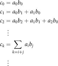
Stevin’s breakthrough allowed polynomials to be treated as numbers and to participate in normal arithmetic operations. To add or subtract polynomials, we simply add or subtract their corresponding coefficients. To multiply, we multiply every combination of elements. That is, if ai and bi are the ith coefficients of the polynomials being multiplied (starting from the lowest-order term) and ci is the ith coefficient of the result, then
To divide polynomials, we need the notion of degree.
Definition 8.1. The degree of a polynomial deg(p) is the index of the highest nonzero coefficient (or equivalently, the highest power of the variable).
For example:
deg(5) = 0
deg(x + 3) = 1
deg(x3 + x – 7) = 3
Now we can define division with remainder:
Definition 8.2. Polynomial a is divisible by polynomial b with remainder r if there are polynomials q and r such that
a = bq + r ∧ deg(r) < deg(b)
(In this equation, q represents the quotient of a ÷ b.)
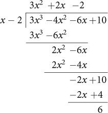
Doing polynomial division with remainder is just like doing long division of numbers:
Exercise 8.2. Prove that for any two polynomials p(x) and q(x):
1. p(x) = q(x) · (x – x0) + r ![]() p(x0) = r
p(x0) = r
2. p(x0) = 0 ![]() p(x) = q(x) · (x – x0)
p(x) = q(x) · (x – x0)
* * *
Stevin realized that he could use the same Euclidean algorithm (the one we looked at in the end of Section 4.6) to compute the GCD of two polynomials; all we really need to do is change the types:
Click here to view code image
polynomial<real> gcd(polynomial<real> a, polynomial<real> b) {
while (b != polynomial<real>(0)) {
a = remainder(a, b);
std::swap(a, b);
}
return a;
}
The remainder function that we use implements the algorithm for polynomial division, although we do not care about the quotient. The polynomial GCD is used extensively in computer algebra for tasks such as symbolic integration.
Stevin’s realization is the essence of generic programming: an algorithm in one domain can be applied in another similar domain.
Just as in Section 4.7, we need to show that the algorithm works—specifically, that it terminates and computes the GCD.
To show that the algorithm terminates, we need to show that it computes the GCD in a finite number of steps. Since it repeatedly performs polynomial remainder, we know by Definition 8.2 that
deg(r) < deg(b)
So at every step, the degree of r is reduced. Since degree is a non-negative integer, the decreasing sequence must be finite.
To show the algorithm computes the GCD, we can use the same argument from Section 4.7; it applies to polynomials as well as integers.
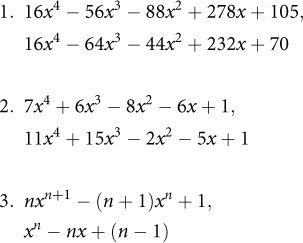
Exercise 8.3 (from Chrystal, Algebra). Find the GCD of the following polynomials:
8.2 Göttingen and German Mathematics
In the 18th and 19th centuries, starting long before Germany existed as a unified country, German culture flourished. Composers like Bach, Mozart, and Beethoven, poets like Goethe and Schiller, and philosophers like Kant, Hegel, and Marx were creating timeless works of depth and beauty. German universities created a unique role for German professors as civil servants bound by their commitment to the truth. Eventually this system would produce the greatest mathematicians and physicists of their age, many of them teaching or studying at the University of Götttingen.
The University of Göttingen
The center of German mathematics was a seemingly unlikely place: the University of Göttingen. Unlike many great European universities that had started hundreds of years earlier in medieval times, Göttingen was relatively young, founded in 1734. And the city of Göttingen was not a major population center. Despite this, the University of Göttingen was home to an astonishing series of top mathematicians, including Gauss, Riemann, Dirichlet, Dedekind, Klein, Minkowski, and Hilbert, some of whom we will discuss later in the book. By the early 20th century its community of physicists was equally impressive, including quantum theorists Max Born and Werner Heisenberg.
Göttingen’s greatness was destroyed in 1933 by the Nazis, who expelled all Jews from the faculty and student body—including many of the top physicists and mathematicians. Some years later, the Nazi Minister of Education asked the great German mathematician David Hilbert, “How is mathematics in Göttingen now that it has been freed of Jewish influence?” Hilbert replied, “Mathematics in Göttingen? There is none any more.”
Perhaps the most important mathematician to come out of Göttingen was Carl Friedrich Gauss, who was the founder of German mathematics in the modern sense. Among his many accomplishments was his seminal work on number theory, described in his 1801 book Disquisitiones Arithmeticae (“Investigations of Arithmetic”). Gauss’s book is to number theory what Euclid’s Elements is to geometry—the foundation on which all later work in the field is based. Among other results, it includes the Fundamental Theorem of Arithmetic, which states that every integer has a unique prime factorization.
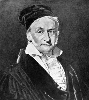
Carl Friedrich Gauss (1777–1855)
Carl Friedrich Gauss grew up in Brunswick, Germany, and was recognized as a child prodigy early in his life. According to a famous story, his elementary school teacher tried to keep the class occupied by asking them to add all the integers from 1 to 100. Nine-year-old Gauss came up with the answer in seconds; he had observed that the first and last numbers added to 101, as did the second and second to last, and so on, so he simply multiplied 101 by 50.
Gauss’s talents came to the attention of the Duke of Brunswick, who paid for the young student’s education starting at age 14, first at a school in his hometown and later at the University of Göttingen. Initially, Gauss considered a career in classics, which, unlike mathematics, was one of the strengths of the university at the time. However, he continued to do mathematics on his own, and in 1796 he made a discovery that had eluded mathematicians since Euclid: how to construct a 17-sided regular polygon using a ruler and a compass. In fact, Gauss went further, proving that construction of a regular p-gon was possible for prime p only if p is a Fermat prime—that is, a number of the form 22k + 1. This breakthrough convinced him to pursue a career in mathematics. In fact, he was so proud of the discovery that he planned to have the 17-gon engraved on his tomb.
In his Ph.D. dissertation, Gauss proved what became known as the Fundamental Theorem of Algebra, which states that every nonconstant polynomial with complex coefficients has a complex root.
Gauss wrote his great number theory treatise, Disquisitiones Arithmeticae, while he was still a student, and had it published in 1801 when he was just 24. While great mathematicians throughout history, such as Euclid, Fermat, and Euler, had worked on number theory, Gauss was the first to codify the field and place it on a formal foundation by introducing modular arithmetic. Disquisitiones is still studied today, and, in fact, some important developments in 20th-century mathematics were the result of careful study of Gauss’s work.
Gauss became world famous in 1801 when he predicted the location of the asteroid Ceres using his method of least squares. Because of this result, he was later appointed director of the astronomical observatory at Göttingen. This pattern of practical problems inspiring his mathematical results continued throughout his career. His work on geodesy (the science of measuring the Earth) led to his invention of the new field of differential geometry. His observations of errors in data led to the idea of the Gaussian distribution in statistics.
Throughout Gauss’s career, he chose his work very carefully, and published only what he considered to be his best results—a small fraction of his potential output. Often he would delay publication, sometimes by years, until he found the perfect way to prove a particular result. His motto was “Few, but ripe.”
Because of the breadth and depth of his contributions, Gauss was known as Princeps Mathematicorum, the Prince of Mathematicians.
Another of Gauss’s innovations was the notion of complex numbers. Mathematicians had used imaginary numbers (xi where i2 = – 1) for over 200 years, but these numbers were not well understood and were usually avoided. The same was true for the first 30 years of Gauss’s career; we have evidence from his notebooks that he used imaginary numbers to derive some of his results, but then he reconstructed the proofs so the published versions would not mention i. (“The metaphysics of i is very complicated,” he wrote in a letter.)
But in 1831, Gauss had a profound insight: he realized that numbers of the form z = x + yi could be viewed as points (x, y) on a Cartesian plane. These complex numbers, he saw, were just as legitimate and self-consistent as any other numbers.
Here are a few definitions and properties we’ll use for complex numbers:
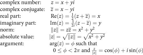
The absolute value of a complex number z is the length of the vector z on the complex plane, while the argument is the angle between the real axis and the vector z. For example, |i| = 1 and arg (i) = 90°.
Just as Stevin did for polynomials, Gauss demonstrated that complex numbers were in fact full-fledged numbers capable of supporting ordinary arithmetic operations:
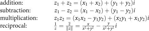
Multiplying two complex numbers can also be done by adding the arguments and multiplying the absolute values. For example, if we want to find ![]() , we know it will also have an absolute value of 1 and an argument of 45° (since 1 · 1 = 1 and 45 + 45 = 90).
, we know it will also have an absolute value of 1 and an argument of 45° (since 1 · 1 = 1 and 45 + 45 = 90).
* * *
Gauss also discovered what are now called Gaussian integers, which are complex numbers with integer coefficients. Gaussian integers have some interesting properties. For example, the Gaussian integer 2 is not prime, since it can be expressed as the product of two other Gaussian integers, 1 + i and 1 – i.
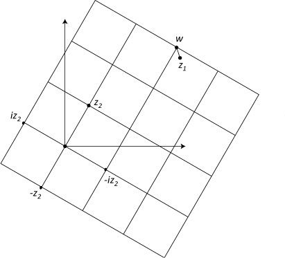
We can’t do full division with Gaussian integers, but we can do division with remainder. To compute the remainder of z1 and z2, Gauss proposed the following procedure:
1. Construct a grid on the complex plane generated by z2, iz2, −iz2, and −z2.
2. Find a square in the grid containing z1.
3. Find a vertex w of the grid square closest to z1.
4. z1 – w is the remainder.
Gauss realized that with this remainder function, he could apply Euclid’s GCD algorithm to complex integers, as we’ve done here:
Click here to view code image
complex<integer> gcd(complex<integer> a, complex<integer> b) {
while (b != complex<integer>(0)) {
a = remainder(a, b);
std::swap(a, b);
}
return a;
}
The only thing we’ve changed are the types.
* * *
Gauss’s work was extended by another Göttingen professor, Peter Gustav Lejeune-Dirichlet. While Gauss’s complex numbers were of the form (in Dirichlet’s terminology) ![]() , Dirichlet realized that this was a special case of
, Dirichlet realized that this was a special case of ![]() where a did not have to be 1, and that different properties followed from the use of different values. For example, the standard GCD algorithm works on numbers of this form when a = 1, but it fails when a = 5 since there end up being numbers that don’t have a unique factorization. For example:
where a did not have to be 1, and that different properties followed from the use of different values. For example, the standard GCD algorithm works on numbers of this form when a = 1, but it fails when a = 5 since there end up being numbers that don’t have a unique factorization. For example:
![]()
It turns out that if Euclid’s algorithm works, then there is a unique factorization. Since we have no unique factorization here, then Euclid’s algorithm doesn’t work in this case.
Dirichlet’s greatest result was his proof that if a and b are coprime (that is, if gcd(a,b) = 1), then there are infinitely many primes of the form ak + b.
Most of Dirichlet’s results were described in the second great book on number theory, appropriately called Vorlesungen über Zahlentheorie (“Lectures on Number Theory”). The book contains the following important insight, which we used in our epigraph for Chapter 4:
[T]he whole structure of number theory rests on a single foundation, namely the algorithm for finding the greatest common divisor of two numbers.
All the subsequent theorems ... are still only simple consequences of the result of this initial investigation....
The book was actually written and published after Dirichlet’s death by his younger Göttingen colleague, Richard Dedekind, based on Dedekind’s notes from Dirichlet’s lectures. Dedekind was so modest that he published the book under Dirichlet’s name, even after adding many additional results of his own in later editions. Unfortunately, Dedekind’s modesty hurt his career; he failed to get tenure at Göttingen and ended up on the faculty of a minor technical university.
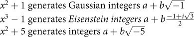
Dedekind observed that Gaussian integers and Dirichlet’s extensions of them were special cases of a more general concept of algebraic integers, which are linear integral combinations of roots of monic polynomials (polynomials where the coefficient of the highest-order term is 1) with integer coefficients. We say that these polynomials generate these sets of algebraic integers. For example:
Dedekind’s work on algebraic integers contained almost all the fundamental building blocks of modern abstract algebra. But it would take another great Göttingen mathematician, Emmy Noether, to make the breakthrough to full abstraction.
8.3 Noether and the Birth of Abstract Algebra
Emmy Noether’s revolutionary insight was that it is possible to derive results about certain kinds of mathematical entities without knowing anything about the entities themselves. In programming terms, we would say that Noether realized that we could use concepts in our algorithms and data structures, without knowing anything about which specific types would be used. In a very real sense, Noether provided the theory for what we now call generic programming. Noether taught mathematicians to always look for the most general setting of any theorem. In a similar way, generic programming defines algorithms in terms of the most general concepts.
Emmy Noether (1882–1935)
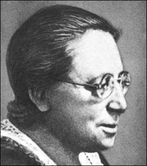
Emmy Noether (pronounced almost like “Nerter,” but without finishing the first “r” sound) was born into an academic German-Jewish family. Her father was a distinguished professor of mathematics at the University of Erlangen. Although it was very unusual for women at the time, Noether was able to study at the university and got a doctorate in mathematics in 1907. She then stayed on for several years at Erlangen, assisting her father and teaching without a position or salary.
Women had been excluded from academic careers for centuries. With the single exception of Sofia Kovalevskaya, a Russian mathematician who became a professor in Stockholm in 1884, there were no women in faculty positions in mathematics at universities at the time.
Two of the greatest mathematicians of the day, Felix Klein and David Hilbert, recognized Noether’s talent, and felt that she deserved an academic position. They also believed as a matter of principle that women should not be excluded from mathematics. They arranged for Noether to come to Göttingen in 1915.
Unfortunately, she still was not officially allowed to teach; the faculty resisted her appointment. For the next four years, all of Noether’s courses were listed under Hilbert’s name; she was treated as a kind of unofficial substitute teacher. Even in 1919, when she was finally given the right to teach under her own name, it was an unpaid position as a Privatdozent, a kind of adjunct professor.
During her time at Göttingen, Noether made enormous contributions in two fields, physics and mathematics. In physics, she is responsible for Noether’s theorem, which fundamentally connected certain symmetries and physical conservation laws (e.g., conservation of angular momentum). Albert Einstein was impressed by Noether’s theorem, which is one of the most profound results in theoretical physics. Her result underlies much of modern physics, from quantum mechanics to the theory of black holes.
In mathematics, Noether created the field of abstract algebra. Although earlier mathematicians such as Cauchy and Galois had worked with groups, rings, and other algebraic objects, they always used specific instances. Noether’s breakthrough was to realize that these algebraic stuctures could be studied abstractly, without looking at particular implementations.
Noether was known as an outstanding teacher, and attracted students from all over the world. Under her leadership, these young researchers (often called “Noether’s Boys”) were creating a new kind of mathematics.
In 1933, when the Nazis expelled Jews from universities, Noether fled to the United States. Despite being one of the greatest mathematicians in the world, no major research university would hire her, primarily because she was a woman. She ended up with a visiting appointment at Bryn Mawr, a small undergraduate women’s college.
Tragically, Emmy Noether died in 1935 at age 53, a few days after surgery to remove an ovarian cyst. Since then, her contributions to mathematics have increasingly been recognized as fundamental and revolutionary.
Noether was well known for her willingness to help students and give them her ideas to publish, but she published relatively little herself. Fortunately, a young Dutch mathematician, Bartel van der Waerden, audited her course and wrote a book based on her lectures (which he credits on the title page). Called Modern Algebra, it was the first book to describe the abstract approach she had developed.
This book, Modern Algebra, led to a fundamental rethinking of the way modern mathematics is presented. Its revolutionary approach—the idea that you express your theorems in the most abstract terms—is Noether’s creation. Most of mathematics—not just algebra—changed as a result of her work; she taught people to think differently.
8.4 Rings
One of Noether’s most important contributions was the development of the theory of an algebraic structure called a ring.4
4 The term “ring,” coined by Hilbert, was intended to use the metaphor of a bunch of people involved in a common enterprise, like a criminal ring. It has nothing to do with jewelry rings.
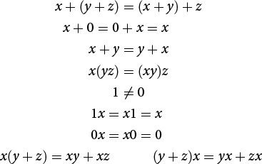
Definition 8.3. A ring is a set on which the following are defined:
operations : x + y, –x, xy
constants : 0R, 1R
and on which the following axioms hold:
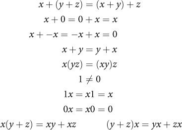
Rings5 have the properties we associate with integer arithmetic—operators that act like addition and multiplication, where addition is commutative and multiplication distributes over addition. Indeed, rings may be thought of as an abstraction of integers, and the canonical example of a ring is the set of integers, ![]() . Also observe that every ring is an additive group and therefore an abelian group. The “addition” operator is required to have an inverse, but the “multiplication” operator is not.
. Also observe that every ring is an additive group and therefore an abelian group. The “addition” operator is required to have an inverse, but the “multiplication” operator is not.
5 Some mathematicians define rings without the multiplicative identity 1 and its axioms, and call rings that include them unitary rings; we do not make that distinction here.
In practice, mathematicians write the zeroes without their subscripts, just as we’ve done in the axioms. For example, in discussing a ring of matrices, “0” refers not to the single integer zero but to the additive identity matrix.
Besides integers, other examples of rings include the following sets:
• n × n matrices with real coefficients
• Gaussian integers
• Polynomials with integer coefficients
We say that a ring is commutative if xy = yx. Noncommutative rings usually come from the realm of linear algebra where matrix multiplication does not commute. In contrast, polynomial rings and rings of algebraic integers do commute. These two types of rings lead to two branches of abstract algebra, known as commutative algebra and noncommutative algebra. Rings are often not explicitly labeled as “commutative” or “noncommutative”; instead, one type of ring or the other is assumed from the branch of algebra. With the exception of Sections 8.5 and 8.6, the rest of this book will deal with commutative algebra—the kind that Dedekind, Hilbert, and Noether worked on—so from then on we will assume our rings are commutative.
Definition 8.4. An element x of a ring is called invertible if there is an element x–1 such that
xx–1 = x–1x = 1
Every ring contains at least one invertible element: 1. There may be more than one; for example, in the ring of integers ![]() , both 1 and –1 are invertible.
, both 1 and –1 are invertible.
Definition 8.5. An invertible element of a ring is called a unit of that ring.
Exercise 8.4 (very easy). Which ring contains exactly one invertible element? What are units in the ring ![]() of Gaussian integers?
of Gaussian integers?
Theorem 8.1: Units are closed under multiplication (i.e., a product of units is a unit).
Proof. Suppose a is a unit and b is a unit. Then (by definition of units) aa–1 = 1 and bb–1 = 1. So
1 = aa–1 = a · 1 · a–1 = a(bb–1)a–1 = (ab)(b–1a–1)
Similarly, a–1a = 1 and b–1b = 1, so
1 = b–1b = b–1 · 1 · b = b–1(a–1a)b = (b–1a–1)(ab)
We now have a term that, when multiplied by ab from either side, gives 1; that term is the inverse of ab:
(ab)–1 = b–1a–1
![]()
So ab is a unit.
Exercise 8.5. Prove that:
• 1 is a unit.
• The inverse of a unit is a unit.
Definition 8.6. An element x of a ring is called a zero divisor if:
1. x ≠ 0
2. There exists a y ≠ 0, xy = 0
For example, in the ring ![]() of remainders modulo 6, 2 and 3 are zero divisors.
of remainders modulo 6, 2 and 3 are zero divisors.
Definition 8.7. A commutative ring is called an integral domain if it has no zero divisors.
It’s called “integral” because its elements act like integers—you don’t get zero when you multiply two nonzero things. Here are some examples of integral domains:
• Integers
• Gaussian integers
• Polynomials over integers
• Rational functions over integers, such as ![]() (A rational function is the ratio of two polynomials.)
(A rational function is the ratio of two polynomials.)
The ring of remainders modulo 6 is not an integral domain. (Whether a ring of remainders is integral depends on whether the modulus is prime.)
Exercise 8.6 (very easy). Prove that a zero divisor is not a unit.
8.5 Matrix Multiplication and Semirings
Note: This section and the next assume some basic knowledge of linear algebra. The rest of the book does not depend on the material covered here, and these sections may be skipped without impacting the reader’s understanding.
In the previous chapter, we combined power with matrix multiplication to compute linear recurrences. It turns out that we can use this technique for many other algorithms if we use a more general notion of matrix multiplication.
Linear Algebra Review
Let’s quickly review how some basic vector and matrix operations are defined.
Inner product of two vectors:
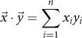
In other words, the inner product is the sum of the products of all the corresponding elements. The result of inner product is always a scalar (a single number).
Matrix-vector product:
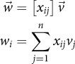
Multiplying an n × m matrix with an m-length vector results in an n-length vector. One way to think of the process is that the ith element of the result is the inner product of the ith row of the matrix with the original vector.
Matrix-matrix product:
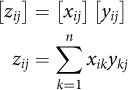
In the matrix product AB = C, if A is a k × m matrix and B is an m × n matrix, then C will be a k × n matrix. The element in row i and column j of C is the inner product of the ith row of A and the jth column of B. Note that matrix multiplication is not commutative: there is no guarantee that AB = BA. Indeed, it’s often the case that only one of AB and BA will be well defined, since the number of columns of the first term has to match the number of rows of the second. Even when both products are defined, they are almost always different.
Just as we generalized our power function to work with any operation, we can now generalize the notion of matrix multiplication. Normally we think of matrix multiplication as consisting of a series of sums of products, as shown in the earlier formula. But what’s mathematically essential is actually that there be two operations, a “plus-like” one that is associative and commutative (denoted by ⊕) and a “times-like” one that is associative (denoted by ⊗), where the latter operation distributes over the first:
a ⊗ (b ⊕ c) = a ⊗ b ⊕ a ⊗ c
(b ⊕ c) ⊗ a = b ⊗ a ⊕ c ⊗ a
We’ve just seen an algebraic structure that has operations like this, a ring. However, rings have a few requirements we don’t need, specifically those involving the additive inverse operation. Instead, what we want is a semiring, a ring without minus (–).
Definition 8.8. A semiring is a set on which the following are defined:
operations : x + y, xy
constants : 0R, 1R
and on which the following axioms hold:
Our definition follows the mathematical convention of referring to the operations as + and × rather than ⊕ and ⊗. But as with all the algebraic structures we’ve been discussing, the symbols refer to any two operations that behave in the manner specified by the axioms.
The canonical example of a semiring is the set of natural numbers ![]() . While natural numbers do not have additive inverses, you can easily perform matrix multiplication on matrices with non-negative integer coefficients. (In fact, we could relax the requirements further by removing the additive identity 0 and the multiplicative identity 1, as well as their corresponding axioms; matrix multiplication6 would still work. We might refer to a semiring without 0 and 1 as a weak semiring.)
. While natural numbers do not have additive inverses, you can easily perform matrix multiplication on matrices with non-negative integer coefficients. (In fact, we could relax the requirements further by removing the additive identity 0 and the multiplicative identity 1, as well as their corresponding axioms; matrix multiplication6 would still work. We might refer to a semiring without 0 and 1 as a weak semiring.)
6 Here we are assuming the straightforward algorithm for matrix multiplication; faster algorithms require stronger theories.
8.6 Application: Social Networks and Shortest Paths
We can use semirings to solve a variety of problems. For example, suppose we have a graph of friendships, as in a social network, and we want to find all the people you are connected to through any path. In other words, we want to know who your friends are, the friends of your friends, the friends of the friends of your friends, and so on.
Finding all such paths is known as finding the transitive closure of the graph. To compute the transitive closure, we take an n × n Boolean matrix where entry xij is 1 if the relation holds between i and j (in this case, if person i is friends with person j), and 0 otherwise; we’ll also assume people are friends with themselves. Here’s a small example:
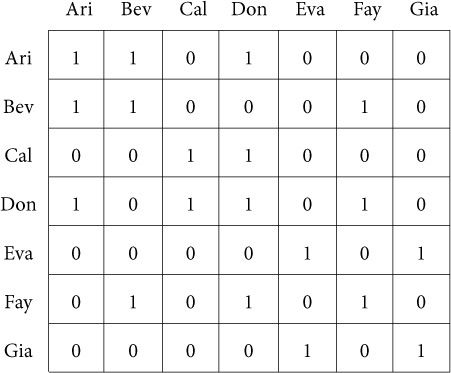
The matrix tells us who each person’s friends are. We can apply generalized matrix multiplication where we replace ⊕ by Boolean OR (∨) and ⊗ by Boolean AND (∧). We say this is the matrix multiplication generated by a Boolean or {∨, ∧}-semiring. Multiplying the matrix by itself using these operations tells us who the friends of our friends are. Doing this multiplication n – 1 times will eventually find all the people in each network of friends. Since multiplying the matrix by itself several times is just raising it to a power, we can use our existing power algorithm to do the computation efficiently. Of course, we can use this idea to compute the transitive closure of any relation.
Exercise 8.7. Using the power algorithm from Chapter 7 with matrix multiplication on Boolean semirings, write a program for finding transitive closure of a graph. Apply this function to find the social networks of each person in the preceding table.
Another example of a classic problem we can solve this way is finding the shortest path between any two nodes in a directed graph like this one:
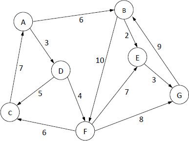
As before, we can represent the graph as an n × n matrix—this time one whose values aij represent the distance from node i to node j. If there is no edge from one node to another, we’ll initially list the distance as infinity.
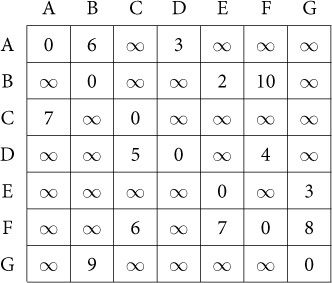
This time, we use matrix multiplication generated by a tropical or {min, +}-semiring:
![]()
That is, the ⊕ operation is min, and the ⊗ operation is +. Again, we raise the resulting matrix to the n – 1 power. The result tells us the shortest path of any length up to n – 1 steps.
Exercise 8.8. Using the power algorithm from Chapter 7 with matrix multiplication on tropical semirings, write a program for finding the length of the shortest path in a graph.
Exercise 8.9. Modify the program from Exercise 8.8 to return not just the shortest distance but the shortest path (a sequence of edges).
8.7 Euclidean Domains
We began this chapter by seeing how Euclid’s GCD algorithm could be generalized beyond integers, first to polynomials, then to complex numbers, and so on. How far could this generalization go? In other words, what are the most general mathematical entities that the GCD algorithm works on (the domain or setting for the algorithm)? With the abstractions Noether had developed, she was finally able answer this question: the domain of the GCD algorithm is what Noether called the Euclidean domain; it is also sometimes known as a Euclidean ring.
Definition 8.9. E is a Euclidean domain if:
• E is an integral domain
• E has operations quotient and remainder such that
b ≠ 0 ![]() a = quotient(a, b) · b + remainder(a, b)
a = quotient(a, b) · b + remainder(a, b)
• E has a non-negative norm ||x||: E → ![]() satisfying
satisfying
The term “norm” here is a measure of magnitude, but it should not be confused with the Euclidean norm you may be familiar with from linear algebra. For integers, the norm is their absolute value; for polynomials, it is the degree of the polynomial; for Gaussian integers, it is the complex norm. The important idea is that when you compute the remainder, the norm decreases and eventually goes to zero, since it maps into natural numbers. We need this property to guarantee that Euclid’s algorithm terminates.
* * *
Now we can write the fully generic version of the GCD algorithm:
Click here to view code image
template <EuclideanDomain E>
E gcd(E a, E b) {
while (b != E(0)) {
a = remainder(a, b);
std::swap(a, b);
}
return a;
}
The process we’ve gone through in transforming the GCD algorithm from something that works only on line segments to something that works on very different types illustrates the following important principle:
To make something generic, you don’t add extra mechanisms. Rather, you remove constraints and strip down the algorithm to its essentials.
8.8 Fields and Other Algebraic Structures
Another important abstraction is the field.7
7 The term “field” relies on the metaphor of a field of study, not a field of wheat.
Definition 8.10. An integral domain where every nonzero element is invertible is called a field.
Just as integers are the canonical example of rings, so rational numbers (![]() ) are the canonical example of fields. Other important examples of fields are as follows:
) are the canonical example of fields. Other important examples of fields are as follows:
• Real numbers ![]()
• Prime remainder fields ![]()
• Complex numbers ![]()
A prime field is a field that does not have a proper subfield (a subfield different from itself). It turns out that every field has one of two kinds of prime subfields: ![]() or
or ![]() . The characteristic of a field is p if its prime subfield is
. The characteristic of a field is p if its prime subfield is ![]() (the field of integer remainders modulo p), and 0 if its prime subfield is
(the field of integer remainders modulo p), and 0 if its prime subfield is ![]() .
.
* * *
All fields can be obtained by starting with a prime field and adding elements that still satisfy the field properties. This is called extending the field.
In particular, we can extend a field algebraically by adding an extra element that is a root of a polynomial. For example, we can extend ![]() with
with ![]() , which is not a rational number, since it is the root of the polynomial x2 – 2.
, which is not a rational number, since it is the root of the polynomial x2 – 2.
We can also extend a field topologically by “filling in the holes.” Rational numbers leave gaps in the number line, but real numbers have no gaps, so the field of real numbers is a topological extension of the field of rational numbers. We can also extend the field to two dimensions with complex numbers. Surprisingly, there are no other finite dimensional fields containing reals.8
8 There are four- and eight-dimensional field-like structures called quaternions and octonions. These are not quite fields, because they are missing certain axioms; both quaternions and octonions lack commutativity of multiplication, and octonions also lack associativity of multiplication. There are no other finite-dimensional extensions of real numbers.
Up to now, every algebraic structure we’ve introduced in this book has operated on a single set of values. But there are also structures that are defined in terms of more than one set. For example, an important structure called a module contains a primary set (an additive group G) and a secondary set (a ring of coefficients R), with an additional multiplication operation R × G → G that obeys the following axioms:
If ring R is also a field, then the structure is called a vector space.
A good example of a vector space is two-dimensional Euclidean space, where the vectors are the additive group and the real coefficients are the field.
8.9 Thoughts on the Chapter
In this chapter, we followed the historical development of generalizing the idea of “numbers” and the corresponding generalization of the GCD algorithm. This led to the development of several new algebraic structures, some of which we used to generalize matrix multiplication and apply it to some important graph problems in computer science.
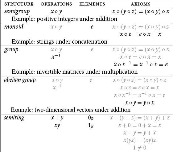
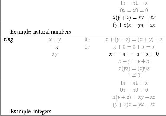
Let’s extend our table from Section 6.8 to include the new structures we introduced in this chapter. Note that every row of the table includes all the axioms from earlier rows. (In the case of semirings and rings, the “times” operation inherits all the axioms from monoids, while the “plus” operation inherits the axioms from abelian groups.) To illustrate this, we’ve grayed out operations, elements, and axioms that appeared previously in the table.
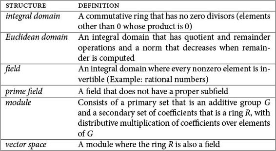
As we did before, we can also define some other structures more concisely in terms of others:
This diagram shows the relationships between some of the most important structures discussed in this chapter:
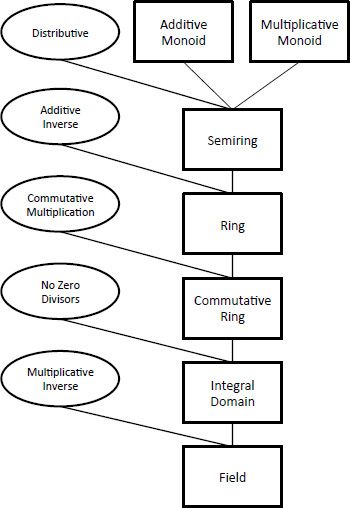
The first time you encounter algebraic structures, it might seem as if there are so many varieties that it’s hard to keep track of their properties. However, they fit into a manageable taxonomy that makes their relationships clear—a taxonomy that has enabled great progress in mathematics over the last hundred years.