Algorithms in a Nutshell 2E (2015)

Chapter 4. Sorting Algorithms

Overview

Numerous computations and tasks become simple by properly sorting information in advance. The search for efficient sorting algorithms dominated the early days of computing. Indeed, much of the early research in algorithms focused on sorting collections of data that were too large for the computers of the day to store in memory. Because computers are incredibly more powerful than the computers of 50 years ago, the size of the data sets being processed is now on the order of terabytes of information. Although you may not be called upon to sort such huge data sets, you will likely need to sort large numbers of items. In this chapter, we cover the most important sorting algorithms and present results from our benchmarks to help you select the best sorting algorithm to use in each situation.

Terminology

A collection of comparable elements A is presented to be sorted in place; we use the notations A[i] and a_i to refer to the i^th element of the collection. By convention, the first element in the collection is A[0]. We use A[low, low+n) to refer to the subcollection A[low] … A[low+n−1] of nelements, whereas A[low, low+n] contains n+1 elements.

To sort a collection, you must reorganize the elements A such that if A[i] < A[j], then i < j. If there are duplicate elements, these elements must be contiguous in the resulting ordered collection; that is, if A[i]=A[j] in a sorted collection, then there can be no k such that i < k < j and A[i]≠A[k]. Finally, the sorted collection A must be a permutation of the elements that originally formed A.

Representation

The collection may already be stored in the computer’s random access memory (RAM), but it might simply exist in a file on the filesystem, known as secondary storage. The collection may be archived in part on tertiary storage (such as tape libraries and optical jukeboxes), which may require extra processing time just to locate the information; in addition, the information may need to be copied to secondary storage (such as hard disk drives) before it can be processed.

Information stored in RAM typically takes one of two forms: pointer-based or value-based. Assume one wants to sort the strings “eagle,” “cat,” “ant,” “dog,” and “ball.” Using pointer-based storage, shown in Figure 4-1, an array of information (i.e., the contiguous boxes) contains pointers to the actual information (i.e., the strings in ovals) rather than storing the information itself. Such an approach enables arbitrarily complex records to be stored and sorted.

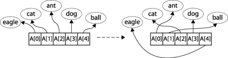
Figure 4-1. Sorting using pointer-based storage

By contrast, value-based storage packs a collection of n elements into record blocks of a fixed size, s, which is better suited for secondary or tertiary storage. Figure 4-2 shows how to store the same information shown in Figure 4-1 using a contiguous block of storage containing a set of rows of exactly s=5 bytes each. In this example the information is shown as strings, but it could be any collection of structured, record-based information. The “¬” character represents a padding character that cannot be part of any string; in this encoding, strings of length s need no padding character. The information is contiguous and can be viewed as a one-dimensional array B[0,n*s). Note that B[r*s + c] is the c^th letter of the r^th word (where c ≥ 0 and r ≥ 0); also, the i^th element of the collection (for i ≥ 0) is the subarray B[i*s,(i+1)*s).

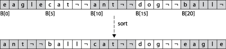
Figure 4-2. Sorting using value-based storage

Information is usually written to secondary storage as a value-based contiguous collection of bytes. The algorithms in this chapter can also be written to work with disk-based information simply by implementing swap functions that transpose bytes within the files on disk; however, the resulting performance will differ because of the increased input/output costs in accessing secondary storage. Merge Sort is particularly well-suited for sorting data in secondary storage.

Whether pointer-based or value-based, a sorting algorithm updates the information (in both cases, the boxes) so that A[0,n) is ordered. For convenience, we use the A[i] notation to represent the i^th element, even when value-based storage is being used.

Comparable Elements

The elements in the collection being compared must admit a total ordering. That is, for any two elements p and q in a collection, exactly one of the following three predicates is true: p=q, p < q, or p > q. Commonly sorted primitive types include integers, floating-point values, and characters. When composite elements are sorted (such as strings of characters), a lexicographical ordering is imposed on each individual element of the composite, thus reducing a complex sort into individual sorts on primitive types. For example, the word “alphabet” is considered to be less than “alternate” but greater than “alligator” by comparing each individual letter, from left to right, until a word runs out of characters or an individual character in one word is different from its partner in the other word (thus “ant” is less than “anthem”).

This question of ordering is far from simple when considering capitalization (is “A” greater than “a”?), diacritical marks (is “è” less than “ê”?) and diphthongs (is “æ” less than “a”?). Note that the powerful Unicode standard (see http://www.unicode.org/versions/latest) uses encodings, such as UTF-16, to represent each individual character using up to four bytes. The Unicode Consortium (see http://www.unicode.org) has developed a sorting standard (known as “the collation algorithm”) that handles the wide variety of ordering rules found in different languages and cultures (Davis and Whistler, 2008).

The algorithms presented in this chapter assume you can provide a comparator function, cmp, which compares elements p to q and returns 0 if p=q, a negative number if p < q, and a positive number if p > q. If the elements are complex records, the cmp function might only compare a “key” value of the elements. For example, an airport terminal might list outbound flights in ascending order of destination city or departure time while flight numbers appear to be unordered.

Stable Sorting

When the comparator function cmp determines that two elements a_i and a_j in the original unordered collection are equal, it may be important to maintain their relative ordering in the sorted set; that is, if i < j, then the final location for a_i must be to the left of the final location for a_j. Sorting algorithms that guarantee this property are considered to be stable. For example, the top of Table 4-1 shows an original collection of flight information already sorted by time of flight during the day (regardless of airline or destination city). If this collection is sorted using a comparator function that orders flights by destination city, one possible result is shown on the bottom of Table 4-1.

You will note that all flights that have the same destination city are sorted also by their scheduled departure time; thus, the sort algorithm exhibited stability on this collection. An unstable algorithm pays no attention to the relationships between element locations in the original collection (it might maintain relative ordering, but it also might not).

Table 4-1. Stable sort of airport terminal information

Criteria for Choosing a Sorting Algorithm

To choose the sorting algorithm to use or implement, consider the qualitative criteria in Table 4-2.

Table 4-2. Criteria for choosing a sorting algorithm

Transposition Sorting

Early sorting algorithms found elements in the collection A that were out of place and moved them into their proper position by transposing (or swapping) elements in A. Selection Sort and (the infamous) Bubble Sort belong to this sorting family. But these algorithms are out-performed byInsertion Sort which we now present.

Insertion Sort

Insertion Sort repeatedly invokes an insert helper function to ensure that A[0,i] is properly sorted; eventually, i reaches the rightmost element, sorting A entirely.

INSERTION SORT SUMMARY

Best: O(n) Average, Worst: O(n²)

sort (A)

for pos = 1 to n-1 do

insert (A, pos, A[pos])

end

insert (A, pos, value)

i = pos - 1

while i >= 0 andA[i] > value do

A[i+1] = A[i]

i = i-1

A[i+1] = value

end

Shifts elements greater than value to the right

Inserts value into proper location

Figure 4-3 shows how Insertion Sort operates on a small, unordered collection A of size n=16. The 15 rows that follow depict the state of A after each pass.

A is sorted in place by incrementing pos=1 up to n−1 and inserting the element A[pos] into its rightful position in the growing sorted region A[0,pos], demarcated on the right by a bold vertical line. The elements shaded in gray were shifted to the right to make way for the inserted element; in total, Insertion Sort executed 60 neighboring transpositions (a movement of just one place by an element).

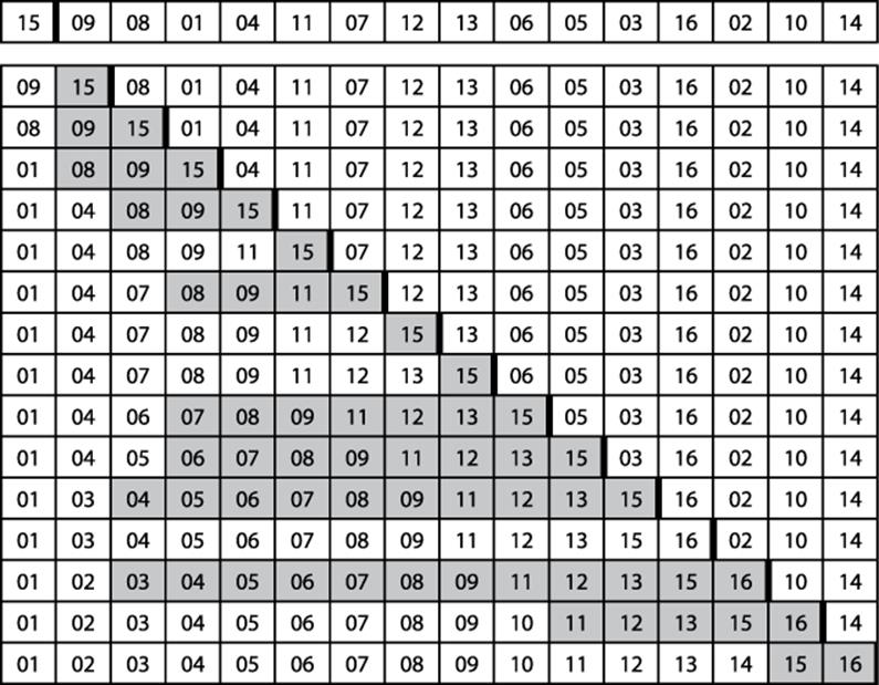
Figure 4-3. The progression of Insertion Sort on a small array

Context

Use Insertion Sort when you have a small number of elements to sort or the elements in the initial collection are already “nearly sorted.” Determining when the array is “small enough” varies from one machine to another and by programming language. Indeed, even the type of element being compared may be significant.

Solution

When the information is stored using pointers, the C program in Example 4-1 sorts an array ar of items that can be compared using a comparison function, cmp.

Example 4-1. Insertion Sort with pointer-based values

void sortPointers (void **ar, int n,

int(*cmp)(const void *, const void *)) {

int j;

for (j = 1; j < n; j++) {

int i = j-1;

void *value = ar[j];

while (i >= 0 && cmp(ar[i], value)> 0) {

ar[i+1] = ar[i];

i--;

}

ar[i+1] = value;

}

}

When A is represented using value-based storage, it is packed into n rows of a fixed element size of s bytes. Manipulating the values requires a comparison function as well as the means to copy values from one location to another. Example 4-2 shows a suitable C program that uses memmoveto transfer the underlying bytes efficiently for a set of contiguous entries in A.

Example 4-2. Insertion Sort using value-based information

void sortValues (void *base, int n, int s,

int(*cmp)(const void *, const void *)) {

int j;

void *saved = malloc (s);

for (j = 1; j < n; j++) {

int i = j-1;

void *value = base + j*s;

while (i >= 0 && cmp(base + i*s, value) > 0) { i--; }

/* If already in place, no movement needed. Otherwise save value

* to be inserted and move as a LARGE block intervening values.

* Then insert into proper position. */

if (++i == j) continue;

memmove (saved, value, s);

memmove (base+(i+1)*s, base+i*s, s*(j-i));

memmove (base+i*s, saved, s);

}

free (saved);

}

The optimal performance occurs when the array is already sorted, and arrays sorted in reverse order produce the worst performance for Insertion Sort. If the array is already mostly sorted, Insertion Sort does well because there is less need to transpose elements.

Insertion Sort requires very little extra space to function; it only needs to reserve space for a single element. For value-based representations, most language libraries offer a block memory move function to make transpositions more efficient.

Analysis

In the best case, each of the n items is in its proper place and thus Insertion Sort takes linear time, or O(n). This may seem to be a trivial point to raise (how often are you going to sort a set of already sorted elements?), but it is important because Insertion Sort is the only comparison-based sorting algorithm that has this behavior.

Much real-world data is already partially sorted, so optimism and realism might coincide to make Insertion Sort an effective algorithm to use. The efficiency of Insertion Sort increases when duplicate items are present, since there are fewer swaps to perform.

Unfortunately, Insertion Sort is too conservative when all n items are distinct and the array is randomly organized (i.e., all permutations of the data are equally likely) because each item starts on average n/3 positions in the array from its final position. The program numTranspositions in the code repository empirically validates this claim for small n up to 12; also see Trivedi (2001). In the average and worst case, each of the n items must be transposed a linear number of positions, thus Insertion Sort requires O(n²) quadratic time.

Insertion Sort operates inefficiently for value-based data because of the amount of memory that must be shifted to make room for a new value. Table 4-3 contains direct comparisons between a naïve implementation of value-based Insertion Sort and the implementation from Example 4-2. Here 10 random trials of sorting n elements were conducted, and the best and worst results were discarded. This table shows the average of the remaining eight runs. Note how the implementation improves by using a block memory move rather than individual memory swapping. Still, as the array size doubles, the performance time approximately quadruples, validating the O(n²) behavior of Insertion Sort. Even with the bulk move improvement, Insertion Sort still remains quadratic.

Table 4-3. Insertion Sort bulk move versus Insertion Sort (in seconds)

When Insertion Sort operates over pointer-based input, swapping elements is more efficient; the compiler can even generate optimized code to minimize costly memory accesses.

Selection Sort

One common sorting strategy is to select the largest value from a collection A and swap its location with the rightmost element A[n-1]. This process is repeated, subsequently, on the leftmost n-1 elements until all values are sorted. This Greedy approach describes Selection Sort, which sorts in place the elements in A[0,n), as shown in Example 4-3.

Example 4-3. Selection Sort implementation in C

static int selectMax (void **ar, int left, int right,

int (*cmp)(const void *, const void *)) {

int maxPos = left;

int i = left;

while (++i <= right) {

if (cmp(ar[i], ar[maxPos])> 0) {

maxPos = i;

}

}

return maxPos;

}

void sortPointers (void **ar, int n,

int(*cmp)(const void *, const void *)) {

/* repeatedly select max in ar[0,i] and swap with proper position */

int i;

for (i = n-1; i >= 1; i--) {

int maxPos = selectMax (ar, 0, i, cmp);

if (maxPos != i) {

void *tmp = ar[i];

ar[i] = ar[maxPos];

ar[maxPos] = tmp;

}

}

}

Selection Sort is the slowest of all the sorting algorithms described in this chapter; it requires quadratic time even in the best case (i.e., when the array is already sorted). It repeatedly performs almost the same task without learning anything from one iteration to the next. Selecting the largest element, max, in A takes n−1 comparisons, and selecting the second largest element, second, takes n−2 comparisons—not much progress! Many of these comparisons are wasted, because if an element is smaller than second, it can’t possibly be the largest element and therefore had no impact on the computation for max. Instead of presenting more details on this poorly performing algorithm, we now consider Heap Sort, which shows how to more effectively apply the principle behind Selection Sort.

Heap Sort

We always need at least n−1 comparisons to find the largest element in an unordered array A of n elements, but can we minimize the number of elements that are compared directly? For example, sports tournaments find the “best” team from a field of n teams without forcing the ultimate winner to play all other n−1 teams. One of the most popular basketball events in the United States is the NCAA championship tournament, where essentially a set of 64 college teams compete for the national title. The ultimate champion team plays five teams before reaching the final determining game, and so that team must win six games. It is no coincidence that 6=log (64). Heap Sort shows how to apply this behavior to sort a set of elements.

HEAP SORT SUMMARY

Best, Average, Worst: O(n log n)

sort (A)

buildHeap (A)

for i = n-1 downto 1 do

swap A[0] with A[i]

heapify (A, 0, i)

end

buildHeap (A)

for i = n/2-1 downto 0 do

heapify (A, i, n)

end

# Recursively enforce that A[idx,max) is valid heap

heapify (A, idx, max)

largest = idx

left = 2*idx + 1

right = 2*idx + 2

if left < max andA[left] > A[idx] then

largest = left

if right < max andA[right] > A[largest] then

largest = right

if largest ≠ idx then

swap A[idx] andA[largest]

heapify (A, largest, max)

end

Assume parent A[idx] is larger than or equal to either of its children

Left child is larger than its parent

Right child is larger than its parent

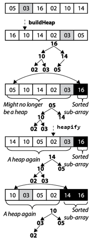
Figure 4-4. Heap Sort example

A heap is a binary tree whose structure ensures two properties:

Shape property

A leaf node at depth k > 0 can exist only if all 2^k−1 nodes at depth k−1 exist. Additionally, nodes at a partially filled level must be added “from left to right.”

Heap property

Each node in the tree contains a value greater than or equal to either of its two children, if it has any.

The sample heap in Figure 4-5(a) satisfies these properties. The root of the binary tree contains the largest element in the tree; however, the smallest element can be found in any leaf node. Although a heap only ensures that a node is greater than either of its children, Heap Sort shows how to take advantage of the shape property to efficiently sort an array of elements.

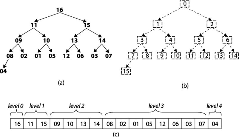
Figure 4-5. (a) Sample heap of 16 unique elements; (b) labels of these elements; (c) heap stored in an array

Given the rigid structure imposed by the shape property, a heap can be stored in an array A without losing any of its structural information. Figure 4-5(b) shows an integer label assigned to each node in the heap. The root is labeled 0. For a node with label i, its left child (should it exist) is labeled 2*i+1; its right child (should it exist) is labeled 2*i+2. Similarly, for a non-root node labeled i, its parent node is labeled ⌊(i-1)/2⌋. Using this labeling scheme, we can store the heap in an array by storing the element value for a node in the array position identified by the node’s label. The array shown in Figure 4-5(c) represents the heap shown in that figure. The order of the elements within A can be simply read from left to right as deeper levels of the tree are explored.

Heap Sort sorts an array by first converting that array in place into a heap. Figure 4-5 shows the results of executing buildHeap on an already sorted array. The progress of buildHeap is shown in Figure 4-6. Each numbered row in this figure shows the result of executing heapify on the initial array from the midway point of ⌊(n/2)⌋−1 down to the leftmost index 0. heapify (A, i, n) updates A to ensure that element A[i] is swapped with the larger of its two children, A[2*i+1] and A[2*i+2], should either one be larger than A[i]. If the swap occurs, heapify recursively checks the grandchildren (and so on) to properly maintain the heap property for A.

As you can see, large numbers are eventually “lifted up” in the resulting heap (which means they are swapped in A with smaller elements to the left). The grayed squares in Figure 4-6 depict the elements swapped in heapify, which is far fewer than the total number of elements swapped inInsertion Sort as depicted in Figure 4-3.

Figure 4-6. buildHeap operating on an initially sorted array

Heap Sort processes an array A of size n by treating it as two distinct subarrays, A[0,m) and A[m, n), which represent a heap of size m and a sorted subarray of n-m elements, respectively. As i iterates from n−1 down to 1, Heap Sort grows the sorted subarray A[i, n) downward by swapping the largest element in the heap (at position A[0]) with A[i]; it then reconstructs A[0,i) to be a valid heap by executing heapify. The resulting non-empty subarray A[i, n) will be sorted because the largest element in the heap represented in A[0,i) is guaranteed to be smaller than any element in the sorted subarray A[i, n).

Context

Heap Sort is not a stable sort. Heap Sort avoids many of the nasty (almost embarrassing!) cases that cause Quicksort to perform badly. Nonetheless, in the average case Quicksort outperforms Heap Sort.

Solution

A sample implementation in C is shown in Example 4-4.

Example 4-4. Heap Sort implementation in C

static void heapify (void **ar, int(*cmp)(const void *, const void *),

int idx, int max) {

int left = 2*idx + 1;

int right = 2*idx + 2;

int largest;

/* Find largest element of A[idx], A[left], and A[right]. */

if (left < max && cmp (ar[left], ar[idx]) > 0) {

largest = left;

} else {

largest = idx;

}

if (right < max && cmp(ar[right], ar[largest]) > 0) {

largest = right;

}

/* If largest is not already the parent then swap and propagate. */

if (largest != idx) {

void *tmp;

tmp = ar[idx];

ar[idx] = ar[largest];

ar[largest] = tmp;

heapify(ar, cmp, largest, max);

}

}

static void buildHeap (void **ar,

int(*cmp)(const void *, const void *), int n) {

int i;

for (i = n/2-1; i>=0; i--) {

heapify (ar, cmp, i, n);

}

}

void sortPointers (void **ar, int n,

int(*cmp)(const void *, const void *)) {

int i;

buildHeap (ar, cmp, n);

for (i = n-1; i >= 1; i--) {

void *tmp;

tmp = ar[0];

ar[0] = ar[i];

ar[i] = tmp;

heapify (ar, cmp, 0, i);

}

}

Analysis

heapify is the central operation in Heap Sort. In buildHeap, it is called ⌊(n/2)⌋−1 times, and during the actual sort it is called n−1 times, for a total of ⌊(3*n/2)⌋−2 times. As you can see, it is a recursive operation that executes a fixed number of computations until the end of the heap is reached. Because of the shape property, the depth of the heap will always be ⌊ log n ⌋ where n is the number of elements in the heap. The resulting performance, therefore, is bounded by (⌊(3*n/2)⌋−2)*⌊ log n ⌋, which is O(n log n).

Variations

The code repository contains a non-recursive Heap Sort implementation and Table 4-4 presents a benchmark comparison on running 1,000 randomized trials of both implementations, discarding the best and worst performances of each.

Table 4-4. Comparing Heap Sort vs. non-recursive Heap Sort (in seconds)

At first, there is a noticeable improvement in eliminating recursion in Heap Sort, but this difference reduces as n increases.

Partition-based Sorting

A Divide and Conquer strategy solves a problem by dividing it into two independent subproblems, each about half the size of the original problem. You can apply this strategy to sorting as follows: find the median element in the collection A and swap it with the middle element of A. Now swap elements in the left half that are greater than A[mid] with elements in the right half that are lesser than or equal to A[mid]. This subdivides the original array into two distinct subarrays that can be recursively sorted in place to sort the original collection A.

Implementing this approach is challenging because it might not be obvious how to compute the median element of a collection without sorting the collection first! It turns out that you can use any element in A to partition A into two subarrays; if you choose “wisely” each time, then both subarrays will be more-or-less the same size and you will achieve an efficient implementation.

Assume there is a function p = partition (A, left, right, pivotIndex) that uses a special pivot value in A, A[pivotIndex], to modify A and return the location p in A such that:

§ A[p]=pivot

§ all elements in A[left,p) are lesser than or equal to pivot

§ all elements in A[p+1,right] are greater than or equal to pivot.

If you are lucky, when partition completes, the size of these two subarrays are more-or-less half the size of the original collection. A C implementation of partition is shown in Example 4-5.

Example 4-5. C implementation to partition ar[left,right] around a given pivot element

/**

* In linear time, group the subarray ar[left, right] around a pivot

* element pivot=ar[pivotIndex] by storing pivot into its proper

* location, store, within the subarray (whose location is returned

* by this function) and ensuring that all ar[left,store) <= pivot and

* all ar[store+1,right] > pivot.

*/

int partition (void **ar, int(*cmp)(const void *, const void *),

int left, int right, int pivotIndex) {

int idx, store;

void *pivot = ar[pivotIndex];

/* move pivot to the end of the array */

void *tmp = ar[right];

ar[right] = ar[pivotIndex];

ar[pivotIndex] = tmp;

/* all values <= pivot are moved to front of array and pivot inserted

* just after them. */

store = left;

for (idx = left; idx < right; idx++) {

if (cmp(ar[idx], pivot) <= 0) {

tmp = ar[idx];

ar[idx] = ar[store];

ar[store] = tmp;

store++;

}

}

tmp = ar[right];

ar[right] = ar[store];

ar[store] = tmp;

return store;

}

The Quicksort algorithm, introduced by C.A.R. Hoare in 1960, selects an element in the collection (sometimes randomly, sometimes the leftmost, sometimes the middle one) to partition an array into two subarrays. Thus Quicksort has two steps. First the array is partitioned and then each subarray is recursively sorted.

QUICKSORT SUMMARY

Best, Average: O(n log n), Worst: O(n²)

sort (A)

quicksort (A, 0, n-1)

end

quicksort (A, left, right)

if left < right then

pi = partition (A, left, right)

quicksort (A, left, pi-1)

quicksort (A, pi+1, right)

end

This pseudocode intentionally doesn’t specify the strategy for selecting the pivot index. In the associated code, we assume there is a selectPivotIndex function that selects an appropriate index. We do not cover here the advanced mathematical analytic tools needed to prove thatQuicksort offers O(n log n) average behavior; further details on this topic are available in (Cormen et al., 2009).

Figure 4-7 shows Quicksort in action. Each of the black squares represents a pivot selection. The first pivot selected is “2”, which turns out to be a poor choice since it produces two subarrays of size 1 and size 14. During the next recursive invocation of Quicksort on the right subarray, “12” is selected to be the pivot, which produces two subarrays of size 9 and 4, respectively. Already you can see the benefit of using partition since the last four elements in the array are, in fact, the largest four elements. Because of the random nature of the pivot selection, different behaviors are possible. In a different execution, shown in Figure 4-8, the first selected pivot nicely subdivides the problem into two more-or-less comparable tasks.

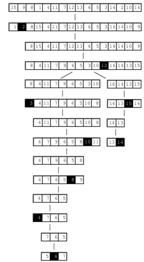
Figure 4-7. Sample Quicksort execution

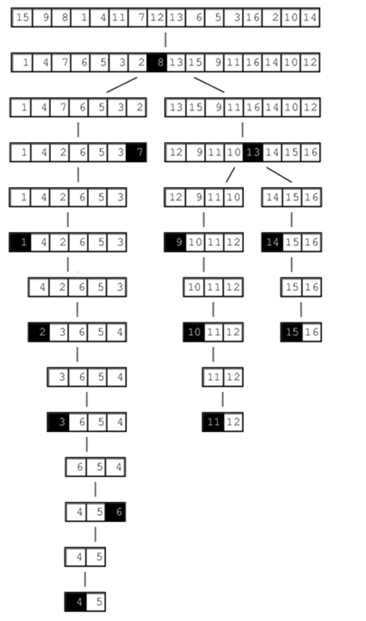
Figure 4-8. A different Quicksort behavior

Context

Quicksort exhibits worst-case quadratic behavior if the partitioning at each recursive step only divides a collection of n elements into an “empty” and “large” set, where one of these sets has no elements and the other has n−1 (note that the pivot element provides the last of the n elements, so no element is lost).

Solution

The Quicksort implementation shown in Example 4-6 includes a standard optimization to use Insertion Sort when the size of the subarray to be sorted falls below a predetermined minimum size.

Example 4-6. Quicksort implementation in C

/**

* Sort array ar[left,right] using Quicksort method.

* The comparison function, cmp, is needed to properly compare elements.

*/

void do_qsort (void **ar, int(*cmp)(const void *, const void *),

int left, int right) {

int pivotIndex;

if (right <= left) { return; }

/* partition */

pivotIndex = selectPivotIndex (ar, left, right);

pivotIndex = partition (ar, cmp, left, right, pivotIndex);

if (pivotIndex-1-left <= minSize) {

insertion (ar, cmp, left, pivotIndex-1);

} else {

do_qsort (ar, cmp, left, pivotIndex-1);

}

if (right-pivotIndex-1 <= minSize) {

insertion (ar, cmp, pivotIndex+1, right);

} else {

do_qsort (ar, cmp, pivotIndex+1, right);

}

}

/** Qsort straight */

void sortPointers (void **vals, int total_elems,

int(*cmp)(const void *, const void *)) {

do_qsort (vals, cmp, 0, total_elems-1);

}

The external method selectPivotIndex(ar, left, right) chooses the pivot value on which to partition the array.

Analysis

Surprisingly, using a random element as pivot enables Quicksort to provide an average-case performance that usually outperforms other sorting algorithms. In addition, there are numerous enhancements and optimizations researched for Quicksort that have wrought the most efficiency out of any sorting algorithm.

In the ideal case, partition divides the original array in half and Quicksort exhibits O(n log n) performance. In practice, Quicksort is effective with a randomly selected pivot.

In the worst case, the largest or smallest item is picked as the pivot. When this happens, Quicksort makes a pass over all elements in the array (in linear time) to sort just a single item in the array. If this process is repeated n−1 times, it will result in O(n²) worst-case behavior.

Variations

Quicksort is the sorting method of choice on most systems. On Unix-based systems, there is a built-in library function called qsort. Often, the operating system uses optimized versions of the default Quicksort algorithm. Two of the commonly cited sources for optimizations are by Sedgewick (1978) and Bentley and McIlroy (1993). It is instructive that some versions of the Linux operating system implement qsort using Heap Sort.

Various optimizations include:

§ Create a stack that stores the subtasks to be processed to eliminate recursion.

§ Choose the pivot based upon median-of-three.

§ Set minimum partition size to use Insertion Sort instead (which varies by implementation and machine architecture; for example, on the Sun4 architecture the minimum value is set to 4 based on empirical evaluation).

§ When processing subarrays, push the larger partition onto the stack first to minimize the total size of the stack by ensuring that the smaller problem is worked on first.

However, none of these optimizations will eliminate the O(n²) worst-case behavior of Quicksort. The only way to ensure an O(n log n) worst-case performance is to use a partition function that can guarantee it finds a “reasonable approximation” to the actual median of that set. The Blum-Floyd-Pratt-Rivest-Tarjan (BFPRT) partition algorithm (Blum et al., 1973) is a provably linear time algorithm, but it has only theoretical value. An implementation of BFPRT is provided with the code repository.

Picking a pivot

Selecting the pivot element from a subarray A[left, left+n) must be an efficient operation; it shouldn’t require checking all n elements of the subarray. Some alternatives are:

§ Select first or last: A[left] or A[left+n−1]

§ Select random element in A[left, left+n−1]

§ Select median-of-k: the middle value of k elements in A[left, left+n−1]

Often one chooses k=3, and, not surprisingly, this variation is known as median-of-three. Sedgewick reports that this approach returns an improvement of 5%, but note that some arrangements of data will force even this alternative into subpar performance (Musser, 1997). A median-of-five pivot selection has also been used. Performing further computation to identify the proper pivot is rarely able to provide beneficial results because of the extra computational costs.

Processing the partition

In the partition method shown in Example 4-5, elements less than or equal to the selected pivot are inserted toward the front of the subarray. This approach might skew the size of the subarrays for the recursive step if the selected pivot has many duplicate elements in the array. One way to reduce the imbalance is to place elements equal to the pivot alternatively in the first subarray and second subarray.

Processing subarrays

Quicksort usually yields two recursive invocations of Quicksort on smaller subarrays. While processing one, the activation record of the other is pushed onto the execution stack. If the larger subarray is processed first, it is possible to have a linear number of activation records on the stack at the same time (although modern compilers may eliminate this observed overhead). To minimize the possible depth of the stack, process the smaller subarray first.

If the depth of the recursion is a foreseeable issue, then perhaps Quicksort is not appropriate for your application. One way to break the impasse is to use a stack data structure to store the set of subproblems to be solved, rather than relying on recursion.

Using simpler insertion sort technique for small subarrays

On small arrays, Insertion Sort is faster than Quicksort, but even when used on large arrays, Quicksort ultimately decomposes the problem to require numerous small subarrays to be sorted. One commonly used technique to improve the recursive performance Quicksort is to invokeQuicksort for large subarrays only, and use Insertion Sort for small ones, as shown in Example 4-6.

Sedgewick (1978) suggests that a combination of median-of-three and using Insertion Sort for small subarrays offers a speedup of 20–25% over pure Quicksort.

IntroSort

Switching to Insertion Sort for small subarrays is a local decision that is made based upon the size of the subarray. Musser (1997) introduced a Quicksort variation called IntroSort, which monitors the recursive depth of Quicksort to ensure efficient processing. If the depth of theQuicksort recursion exceeds log (n) levels, then IntroSort switches to Heap Sort. The SGI implementation of the C++ Standard Template Library uses IntroSort as its default sorting mechanism (http://www.sgi.com/tech/stl/sort.html).

Sorting Without Comparisons

At the end of this chapter, we will show that no comparison-based sorting algorithm can sort n elements in better than O(n log n) performance. Surprisingly, there are potentially faster ways to sort elements if you know something about those elements in advance. For example, if you have a fast hashing function that uniformly partitions a collection of elements into distinct, ordered buckets, you can use the following Bucket Sort algorithm for linear O(n) performance.

Bucket Sort

Given a set of n elements, Bucket Sort constructs a set of n ordered buckets into which the elements of the input set are partitioned; Bucket Sort reduces its processing costs at the expense of this extra space. If a hash function, hash(A[i]), can uniformly partition the input set of n elements into these n buckets, Bucket Sort can sort, in the worst case, in O(n) time. Use Bucket Sort when the following two properties hold:

Uniform distribution

The input data must be uniformly distributed for a given range. Based on this distribution, n buckets are created to evenly partition the input range.

Ordered hash function

The buckets are ordered. If i < j, elements inserted into bucket b_i are lexicographically smaller than elements in bucket b_j.

BUCKET SORT SUMMARY

Best, Average, Worst: O(n)

sort (A)

create n buckets B

for i = 0 to n-1 do

k = hash(A[i])

add A[i] to the k-th bucket B[k]

extract (B, A)

end

extract (B, A)

idx = 0

for i = 0 to n-1 do

insertionSort(B[i])

foreach element e in B[i]

A[idx++] = e

end

Hashing distributes elements evenly to buckets

If more than one element in bucket, sort first

copy elements back into proper position in A.

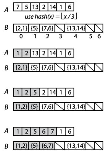
Figure 4-9. Small Example Demonstrating Bucket Sort

Bucket Sort is not appropriate for sorting arbitrary strings, for example, because typically it is impossible to develop a hash function with the required characteristics. However, it could be used to sort a set of uniformly distributed floating-point numbers in the range [0,1).

Once all elements to be sorted are inserted into the buckets, Bucket Sort extracts the values from left to right using Insertion Sort on the contents of each bucket. This orders the elements in each respective bucket as the values from the buckets are extracted from left to right to repopulate the original array.

Solution

In the C implementation for Bucket Sort, shown in Example 4-7, each bucket stores a linked list of elements that were hashed to that bucket. The functions numBuckets and hash are provided externally, based upon the input set.

Example 4-7. Bucket Sort implementation in C

extern int hash(void *elt);

extern int numBuckets(int numElements);

/* linked list of elements in bucket. */

typedef struct entry {

void *element;

struct entry *next;

} ENTRY;

/* maintain count of entries in each bucket and pointer to its first entry */

typedef struct {

int size;

ENTRY *head;

} BUCKET;

/* Allocation of buckets and the number of buckets allocated */

static BUCKET *buckets = 0;

static int num = 0;

/** One by one remove and overwrite ar */

void extract (BUCKET *buckets, int(*cmp)(const void *, const void *),

void **ar, int n) {

int i, low;

int idx = 0;

for (i = 0; i < num; i++) {

ENTRY *ptr, *tmp;

if (buckets[i].size == 0) continue; /* empty bucket */

ptr = buckets[i].head;

if (buckets[i].size == 1) {

ar[idx++] = ptr->element;

free (ptr);

buckets[i].size = 0;

continue;

}

/* insertion sort where elements are drawn from linked list and

* inserted into array. Linked lists are released. */

low = idx;

ar[idx++] = ptr->element;

tmp = ptr;

ptr = ptr->next;

free (tmp);

while (ptr != NULL) {

int i = idx-1;

while (i >= low && cmp (ar[i], ptr->element) > 0) {

ar[i+1] = ar[i];

i--;

}

ar[i+1] = ptr->element;

tmp = ptr;

ptr = ptr->next;

free(tmp);

idx++;

}

buckets[i].size = 0;

}

}

void sortPointers (void **ar, int n,

int(*cmp)(const void *, const void *)) {

int i;

num = numBuckets(n);

buckets = (BUCKET *) calloc (num, sizeof (BUCKET));

for (i = 0; i < n; i++) {

int k = hash(ar[i]);

/** Insert each element and increment counts */

ENTRY *e = (ENTRY *) calloc (1, sizeof (ENTRY));

e->element = ar[i];

if (buckets[k].head == NULL) {

buckets[k].head = e;

} else {

e->next = buckets[k].head;

buckets[k].head = e;

}

buckets[k].size++;

}

/* now sort, read out, and overwrite ar. */

extract (buckets, cmp, ar, n);

free (buckets);

}

For numbers drawn uniformly from [0,1), Example 4-8 contains sample implementations of the hash and numBuckets functions to use.

Example 4-8. hash and numBuckets functions for [0,1) range

static int num;

/** Number of buckets to use is the same as the number of elements. */

int numBuckets(int numElements) {

num = numElements;

return numElements;

}

/**

* Hash function to identify bucket number from element. Customized

* to properly encode elements in order within the buckets. Range of

* numbers is from [0,1), so we subdivide into buckets of size 1/num;

*/

int hash(double *d) {

int bucket = num*(*d);

return bucket;

}

The buckets could also be stored using fixed arrays that are reallocated when the buckets become full, but the linked list implementation is about 30-40% faster.

Analysis

The sortPointers function of Example 4-7 sorts each element from the input into its associated bucket based upon the provided hash function; this takes or O(n) time. Because of the careful design of the hash function, we know that all elements in bucket b_i are smaller than the elements in bucket b_j if i < j.

As the values are extracted from the buckets and written back into the input array, Insertion Sort is used when a bucket contains more than a single element. For Bucket Sort to exhibit O(n) behavior, we must guarantee that the total time to sort each of these buckets is also O(n). Let’s definen_i to be the number of elements partitioned in bucket b_i. We can treat n_i as a random variable (using statistical theory). Now consider the expected value E[n_i] for each bucket b_i. Each element in the input set has probability p=1/n of being inserted into a given bucket because each of these elements is uniformly drawn from the range [0,1). Therefore, E[n_i]=n*p=n*(1/n)=1, while the variance Var[n_i]=n*p*(1-p)=(1-1/n). It is important to consider the variance because some buckets will be empty, and others may have more than one element; we need to be sure that no bucket has too many elements. Once again, we resort to statistical theory, which provides the following equation for random variables:

E[n_i²] = Var[n_i] + E²[n_i]

From this equation we can compute the expected value of n_i². This is critical because it is the factor that determines the cost of Insertion Sort, which runs in a worst case of O(n²). We compute E[n_i²]=(1-1/n)+1=(2-1/n), which shows that E[n_i²] can be considered a constant. This means that when we sum up the costs of executing Insertion Sort on all n buckets, the expected performance cost remains O(n).

Variations

Instead of creating n buckets, Hash Sort creates a suitably large number of buckets k into which the elements are partitioned; as k grows in size, the performance of Hash Sort improves. The key to Hash Sort is a hashing function hash(e) that returns an integer for each element e such thathash(a_i) ≤ hash(a_j) if a_i is lexicographically smaller than a_j.

The hash function hash(e) defined in Example 4-9 operates over elements containing just lowercase letters. It converts the first three characters of the string (using base 26 representation) into an integer value; for the string “abcdefgh,” its first three characters (“abc”) are extracted and converted into the value 0*676+1*26+2=28. This string is thus inserted into the bucket labeled 28.

Example 4-9. hash and numBuckets functions for Hash Sort

/** Number of buckets to use. */

int numBuckets(int numElements) {

return 26*26*26;

}

/**

* Hash function to identify bucket number from element. Customized

* to properly encode elements in order within the buckets.

*/

int hash(void *elt) {

return (((char*)elt)[0] - 'a')*676 +

(((char*)elt)[1] - 'a')*26 +

(((char*)elt)[2] - 'a');

}

The performance of Hash Sort for various bucket sizes and input sets is shown in Table 4-5. We show comparable sorting times for Quicksort using the median-of-three approach for selecting the pivotIndex.

Table 4-5. Sample performance for Hash Sort with different numbers of buckets, compared with Quicksort (in seconds)

Note that with 17,576 buckets, Hash Sort outperforms Quicksort for n>8,192 items (and this trend continues with increasing n). However, with only 676 buckets, once n>32,768 (for an average of 48 elements per bucket), Hash Sort begins its inevitable slowdown with the accumulated cost of executing Insertion Sort on increasingly larger sets. Indeed, with only 26 buckets, once n>256, Hash Sort begins to quadruple its performance as the problem size doubles, showing how too few buckets leads to O(n²) performance.

Sorting with Extra Storage

The sorting algorithms in this chapter all sort a collection in place without requiring any noticeable extra storage. We now present Merge Sort, which offers O(n log n) behavior in the worst case and can be used to efficiently sort data that is stored externally in a file.

Merge Sort

To sort a collection A, divide it evenly into two smaller collections, each of which is then sorted. A final phase merges these two sorted collections back into a single collection of size n. A naive implementation of this approach, shown below, uses far too much extra storage.

sort (A)

if A has less than 2 elements then

return A

else if A has 2 elements then

swap elements of A if out of order

return A

sub1 = sort(left half of A)

sub2 = sort(right half of A)

merge sub1 andsub2 into new array B

return B

end

Each recursive call of sort will require space equivalent to the size of the array, or O(n) and there will be O(log n) such recursive calls, thus the storage requirement for this naive implementation is O(n log n). Fortunately there is a way to use only O(n) storage, as we now discuss.

MERGE SORT SUMMARY

Best, Average, Worst: O(n log n)

sort (A)

copy = copy of A

mergeSort (copy, A, 0, n)

end

mergeSort (A, result, start, end)

if end - start < 2 then return

if end - start = 2 then

swap elements of result if out of order

return

mid = (start + end)/2;

mergeSort(result, A, start, mid);

mergeSort(result, A, mid, end);

merge left andright halves of A into result

end

Make full copy of all elements

Place sorted A[start,end) into result[start,end)

Sort region of result and leave corresponding output in A

Each recursive call alternates storage in A or copy

Input/Output

The output of the sort is returned in place within the original collection A. The internal storage copy is discarded.

Solution

Merge Sort merges the left- and right- sorted subarrays using two indices i and j to iterate over the left (and right) elements, always copying the smaller of A[i] and A[j] into its proper location result[idx]. There are three cases to consider:

§ The right side is exhausted (j ≥ end), in which case the remaining elements are taken from the left side

§ The left side is exhausted (i ≥ mid), in which case the remaining elements are taken from from the right side

§ The left and right side have elements; if A[i] < A[j], insert A[i] otherwise insert A[j]

Once the for loop completes, result has the merged (and sorted) elements from the original A[start, end). Example 4-10 contains the Python implementation.

Example 4-10. Merge Sort implementation in Python

def sort (A):

"""merge sort A in place."""

copy = list(A)

mergesort_array (copy, A, 0, len(A))

def mergesort_array(A, result, start, end):

"""Mergesort array in memory with given range."""

if end - start < 2:

return

if end - start == 2:

if result[start] > result[start+1]:

result[start],result[start+1] = result[start+1],result[start]

return

mid = (end + start) // 2

mergesort_array(result, A, start, mid)

mergesort_array(result, A, mid, end)

# merge A left- and right- side

i = start

j = mid

idx = start

while idx < end:

if j >= end or (i < mid andA[i] < A[j]):

result[idx] = A[i]

i += 1

else:

result[idx] = A[j]

j += 1

idx += 1

Analysis

This algorithm must complete the “merge” phase in O(n) time after recursively sorting the left- and right-half of the range A[start, end), placing the properly ordered elements in the array referenced as result.

Because copy is a true copy of the entire array A, the terminating base cases of the recursion will work because they reference the original elements of the array directly at their respective index locations. This observation is a sophisticated one and is the key to the algorithm. In addition, the final merge step requires only O(n) operations, which ensures the total performance remains O(n log n). Because copy is the only extra space used by the algorithm, the total space requirements are O(n).

Variations

Of all the sorting algorithms, Merge Sort is the easiest one to convert to working with external data. Example 4-11 contains a full Java implementation using memory-mapping of data to efficiently sort a file containing binary-encoded integers. This sorting algorithm requires the elements to all have the same size, so it can’t easily be adapted to sort arbitrary strings or other variable-length elements.

Example 4-11. External Merge Sort implementation in Java

public static void mergesort (File A) throws IOException {

File copy = File.createTempFile("Mergesort", ".bin");

copyFile(A, copy);

RandomAccessFile src = new RandomAccessFile(A, "rw");

RandomAccessFile dest = new RandomAccessFile(copy, "rw");

FileChannel srcC = src.getChannel();

FileChannel destC = dest.getChannel();

MappedByteBuffer srcMap = srcC.map(FileChannel.MapMode.READ_WRITE,

0, src.length());

MappedByteBuffer destMap = destC.map(FileChannel.MapMode.READ_WRITE,

0, dest.length());

mergesort (destMap, srcMap, 0, (int) A.length());

// The following two invocations are only needed on Windows Platform

closeDirectBuffer(srcMap);

closeDirectBuffer(destMap);

src.close();

dest.close();

copy.deleteOnExit();

}

static void mergesort(MappedByteBuffer A, MappedByteBuffer result,

int start, int end) throws IOException {

if (end - start < 8) {

return;

}

if (end - start == 8) {

result.position(start);

int left = result.getInt();

int right = result.getInt();

if (left > right) {

result.position(start);

result.putInt(right);

result.putInt(left);

}

return;

}

int mid = (end + start)/8*4;

mergesort(result, A, start, mid);

mergesort(result, A, mid, end);

result.position(start);

for (int i = start, j = mid, idx=start; idx < end; idx += 4) {

int Ai = A.getInt(i);

int Aj = 0;

if (j < end) { Aj = A.getInt(j); }

if (j >= end || (i < mid && Ai < Aj)) {

result.putInt(Ai);

i += 4;

} else {

result.putInt(Aj);

j += 4;

}

}

}

The structure is identical to the Merge Sort implementation, but it uses a memory-mapped structure to efficiently process data stored on the file system. There are issues on Windows operating systems that fail to properly close the MappedByteBuffer data. The repository contains a work-around method closeDirectBuffer(MappedByteBuffer) that will handle this responsibility.

String Benchmark Results

To choose the appropriate algorithm for different data, you need to know some properties about your input data. We created several benchmark data sets on which to show how the algorithms presented in this chapter compare with one another. Note that the actual values of the generated tables are less important because they reflect the specific hardware on which the benchmarks were run. Instead, you should pay attention to the relative performance of the algorithms on the corresponding data sets:

Random strings

Throughout this chapter, we have demonstrated performance of sorting algorithms when sorting 26-character strings that are permutations of the letters in the alphabet. Given there are n! such strings, or roughly 4.03*10²⁶ strings, there are few duplicate strings in our sample data sets. In addition, the cost of comparing elements is not constant, because of the occasional need to compare multiple characters.

Double precision floating-point values

Using available pseudorandom generators available on most operating systems, we generate a set of random numbers from the range [0,1). There are essentially no duplicate values in the sample data set and the cost of comparing two elements is a fixed constant. Results on these data sets are not included here, but can be found in the code repository.

The input data provided to the sorting algorithms can be preprocessed to ensure some of the following properties (not all are compatible):

Sorted

The input elements can be presorted into ascending order (the ultimate goal) or in descending order.

Killer median-of-three

Musser (1997) discovered an ordering that ensures that Quicksort requires O(n²) comparisons when using median-of-three to choose a pivot.

Nearly sorted

Given a set of sorted data, we can select k pairs of elements to swap and the distance d with which to swap (or 0 if any two pairs can be swapped). Using this capability, you can construct input sets that might more closely match your input set.

The upcoming tables are ordered left to right, based upon how well the algorithms perform on the final row in the table. Each section has four tables, showing performance results under the four different situations outlined earlier in this chapter.

To produce the results shown in Table 4-6 through [Link to Come], we executed each trial 100 times and discarded the best and worst performers. The average of the remaining 98 trials is shown in these tables. The columns labeled Quicksort BFPRT⁴ minSize=4 refer to a Quicksortimplementation that uses BFPRT (with groups of 4) to select the partition value and which switches to Insertion Sort when a subarray to be sorted has four or fewer elements.

Table 4-6. Performance results (in seconds) on random 26-letter permutations of the alphabet

Table 4-7. Performance (in seconds) on sorted random 26-letter permutations of the alphabet

Because the performance of Quicksort median-of-three degrades so quickly, only 10 trials were executed in Table 4-8.

Table 4-8. Performance (in seconds) on killer median data

Analysis Techniques

When analyzing a sorting algorithm, one must explain its best-case, worst-case, and average-case performance (as discussed in Chapter 2). The average case is typically hardest to accurately quantify and relies on advanced mathematical techniques and estimation. Also, it assumes a reasonable understanding of the likelihood that the input may be partially sorted. Even when an algorithm has been shown to have a desirable average-case cost, its implementation may simply be impractical. Each sorting algorithm in this chapter is analyzed both by its theoretical behavior and by its actual behavior in practice.

A fundamental result in computer science is that no algorithm that sorts by comparing elements can do better than O(n log n) performance in the average or worst case. We now sketch a proof. Given n items, there are n! permutations of these elements. Every algorithm that sorts by pairwise comparisons corresponds to a binary decision tree. The leaves of the tree correspond to an underlying permutation, and every permutation must have at least one leaf in the tree. The nodes on a path from the root to a leaf correspond to a sequence of comparisons. The height of such a tree is the number of comparison nodes in the longest path from the root to a leaf node; for example, the height of the tree in Figure 4-10 is 5 because only five comparisons are needed in all cases (although in four cases only four comparisons are needed).

Construct a binary decision tree where each internal node of the tree represents a comparison a_i ≤ a_j and the leaves of the tree represent one of the n! permutations. To sort a set of n elements, start at the root and evaluate the statements shown in each node. Traverse to the left child when the statement is true; otherwise, traverse to the right child. Figure 4-10 shows a sample decision tree for four elements.

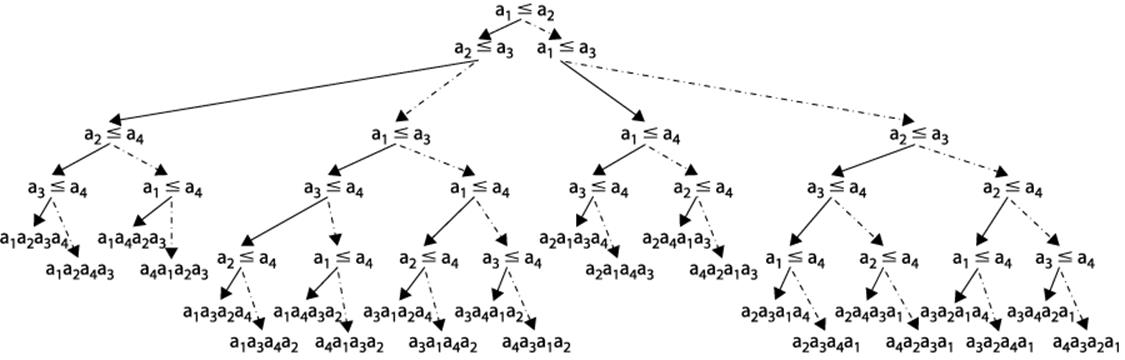
Figure 4-10. Binary decision tree for ordering four elements

One could construct many different binary decision trees. Nonetheless, we assert that given any such binary decision tree for comparing n elements, we can compute its minimum height h; that is, there must be some leaf node that requires h comparison nodes in the tree from the root to that leaf. Consider a complete binary tree of height h in which all non-leaf nodes have both a left and right child. This tree contains a total of n = 2^h − 1 nodes and height h=log (n+1); if the tree is not complete, it could be unbalanced in strange ways, but we know that h ≥ ⌈log (n+1)⌉. Any binary decision tree with n! leaf nodes already demonstrates it has at least n! nodes in total. We need only compute h=⌈log (n!)⌉ to determine the height of any such binary decision tree. We take advantage of the following properties of logarithms: log (a*b)=log (a)+log (b) and log (x y)=y*log (x).

h = log (n!) = log(n * (n−1) * (n−2) * … * 2 * 1)

h > log(n * (n−1) * (n−2) * … * n/2)

h > log((n/2)n/2)

h > (n/2) * log(n/2)

h > (n/2) * (log(n) −1)

Thus h > (n/2)*(log(n)-1). What does this mean? Well, given n elements to be sorted, there will be at least one path from the root to a leaf of size h, which means that an algorithm that sorts by comparison requires at least this many comparisons to sort the n elements. Note that h is computed by a function f(n); here in particular, f(n)=(1/2)*n*log(n)-n/2, which means that any sorting algorithm using comparisons will require O(n log n) comparisons to sort.

References

Bentley, Jon Louis and M. Douglas McIlroy, “Engineering a Sort Function,” Software—Practice and Experience, 23(11): 1249–1265, 1993, http://citeseer.ist.psu.edu/bentley93engineering.html.

Blum, Manuel, Robert Floyd, Vaughan Pratt, Ronald Rivest, and Robert Tarjan, “Time bounds for selection.” Journal of Computer and System Sciences, 7(4): 448–461, 1973.

Cormen, Thomas H., Charles E. Leiserson, Ronald L. Rivest, and Clifford Stein, Introduction to Algorithms, Second Edition. McGraw-Hill, 2001.

Davis, Mark and Ken Whistler, “Unicode Collation Algorithm, Unicode Technical Standard #10,” March 2008, http://unicode.org/reports/tr10/.

Gilreath, William, “Hash sort: A linear time complexity multiple-dimensional sort algorithm.” Proceedings of First Southern Symposium on Computing, December 1998, http://www.citebase.org/abstract?id=oai:arXiv.org:cs/0408040=oai:arXiv.org:cs/0408040.

Musser, David, “Introspective sorting and selection algorithms.” Software—Practice and Experience, 27(8): 983–993, 1997.

Sedgewick, Robert, “Implementing Quicksort Programs.” Communications ACM, 21: 847–857, 1978.

Trivedi, Kishor Shridharbhai, Probability and Statistics with Reliability, Queueing, and Computer Science Applications, Second Edition. Wiley-Interscience Publishing, 2001.