Algorithms in a Nutshell 2E (2015)

Chapter 6. Graph Algorithms

Graphs are fundamental structures that represent complex structured information. The images in Figure 6-1 are all sample graphs.

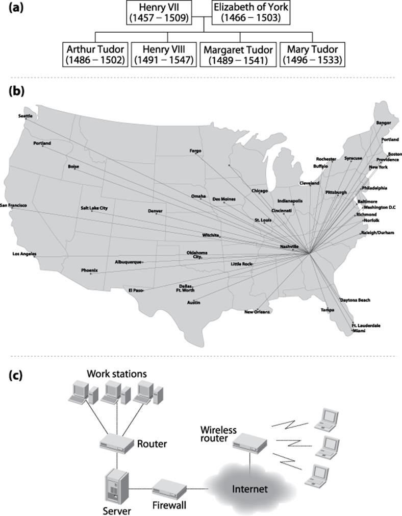
Figure 6-1. (a) House of Tudor, (b) airline schedule, (c) computer network. (NEED BETTER EXAMPLES)

In this chapter we investigate common ways to represent graphs and associated algorithms that frequently occur. Inherently, a graph contains a set of elements, known as vertices and relationships between pairs of these elements, known as edges. We use these terms consistently in this chapter; other descriptions might use the terms “node” and “link” to represent the same information. We consider only simple graphs that avoid (a) self-edges from a vertex to itself, and (b) multiple edges between the same pair of vertices.

Given the structure defined by the edges in a graph, many problems can be stated in terms of the shortest path that exists between two vertices in the graph, where the length of a path is the sum of the lengths of the edges of that path. In the Single Source Shortest Path algorithm, one is given a specific vertex, s, and asked to compute the shortest path to all other vertices in the graph. The All Pairs Shortest Path problem requires that the shortest path be computed for all pairs (u, v) of vertices in the graph.

Some problems seek a deeper understanding of the underlying graph structure. For example, the minimum spanning tree (MST) of an undirected, weighted graph is a subset of that graph’s edges such that (a) the original set of vertices is still connected in the MST, and (b) the sum total of the weights of the edges in the MST is minimum. We show how to efficiently solve this problem using Prim’s Algorithm.

Graphs

A graph G = (V, E) is defined by a set of vertices, V, and a set of edges, E, over pairs of these vertices. There are three common types of graphs:

Undirected, unweighted graphs

These model relationships between vertices (u, v) without regard for the direction of the relationship. These graphs are useful for capturing symmetric information. For example, a road from town A to town B can be traversed in either direction.

Directed graphs

These model relationships between vertices (u, v) that are distinct from the relationship between (v, u), which may or may not exist. For example, a program to provide driving directions must store information on one-way streets to avoid giving illegal directions.

Weighted graphs

These model relationships where there is a numeric value known as a weight associated with the relationship between vertices (u, v). Sometimes these values can store arbitrary non-numeric information. For example, the edge between towns A and B could store the mileage between the towns; alternatively, it could store estimated traveling time in minutes.

The most highly structured of the graphs—a directed, weighted graph—defines a non-empty set of vertices {v₀, v₁, …, v_n−1}, a set of directed edges between pairs of distinct vertices (such that every pair has at most one edge between them in each direction), and a positive weight associated with each edge. In many applications, the weight is considered to be a distance or cost. For some applications, we may want to relax the restriction that the weight must be positive (for example, a negative weight could reflect a loss, not a profit), but we will be careful to declare when this happens.

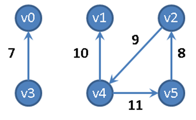
Figure 6-2. Sample directed, weighted graph

Consider the directed, weighted graph in Figure 6-2, which is composed of six vertices and five edges. One could store the graph using adjacency lists, as shown in Figure 6-3, where each vertex v_i maintains a linked list of nodes, each of which stores the weight of the edge leading to an adjacent vertex of v_i. Thus the base structure is a one-dimensional array of vertices in the graph.

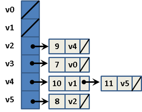
Figure 6-3. Adjacency list representation of directed, weighted graph

Figure 6-4 shows how to store the directed, weighted graph as an n-by-n adjacency matrix A of integers, indexed in both dimensions by the vertices. The entry A[i][j] stores the weight of the edge from v_i to v_j; when A[i][j] = 0, there is no edge from v_i to v_j. We can use adjacency lists and matrices to store non-weighted graphs as well (perhaps using the value 1 to represent an edge). With the adjacency matrix representation, you can add an edge in constant time. You should use this representation when working with dense graphs in which nearly every possible edge exists.

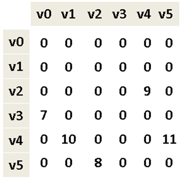
Figure 6-4. Adjacency matrix representation of directed, weighted graph

We use the notation <v₀, v₁, …, v_k−1> to describe a path of k vertices in a graph that traverses k−1 edges (v_i, v_i+1) for 0 ≤ i < k−1; paths in a directed graph honor the direction of the edge. In Figure 6-2, the path <v₄, v₅, v₂, v₄, v₁> is valid. In this graph there is a cycle, which is a path of vertices that includes the same vertex multiple times. A cycle is typically represented in its most minimal form.

When using an adjacency list to store an undirected graph, the same edge (u, v) appears twice: once in the linked list of neighbor vertices for u and once for v. Thus, undirected graphs may require up to twice as much storage in an adjacency list as a directed graph with the same number of vertices and edges. When using an adjacency matrix to store an undirected graph, entry A[i][j]=A[j][i]. If a path exists between any two pairs of vertices in a graph, then that graph is connected.

Data Structure Design

We implement a C++ Graph class to store a directed (or undirected) graph using an adjacency list representation implemented with core classes from the C++ Standard Template Library (STL). Specifically, it stores the information as an array of list objects, one list for each vertex. For each vertex u there is a list of IntegerPair objects representing the edge (u, v) of weight w.

The operations on graphs are subdivided into several categories:

Create

A graph can be initially constructed from a set of n vertices, and it may be directed or undirected. When a graph is undirected, adding edge (u, v) also adds edge (v, u).

Inspect

One can determine whether a graph is directed, find all outgoing edges for a given vertex, determine whether a specific edge exists, and determine the weight associated with an edge. One can construct an iterator that returns the neighboring edges (and their weights) for any vertex in a graph.

Update

One can add edges to (or remove edges from) a graph. It is also possible to add a vertex to (or remove a vertex from) a graph, but algorithms in this chapter do not need to add or remove vertices.

We begin by discussing ways to explore a graph. Two common search strategies are Depth-First Search and Breadth-First Search.

Depth-First Search

Consider the maze shown on the left in Figure 6-5. After some practice, a child can rapidly find the path that stretches from the start box labeled s to the target box labeled t. One way to solve this problem is to make as much forward progress as possible and randomly select a direction whenever a choice is possible, marking where you have come from. If you ever reach a dead end or you revisit a location you have already seen, then backtrack until an untraveled branch is found and set off in that direction. The numbers on the right side of Figure 6-5 reflect the branching points of one such solution; in fact, every square in the maze is visited in this solution.

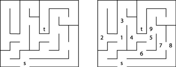
Figure 6-5. A small maze to get from s to t

We can represent the maze in Figure 6-5 by creating a graph consisting of vertices and edges. A vertex is created for each branching point in the maze (labeled by numbers on the right in Figure 6-5), as well as “dead ends.” An edge exists only if there is a direct path in the maze between the two vertices where no choice in direction can be made. The undirected graph representation of the maze from Figure 6-5 is shown in Figure 6-6; each vertex has a unique identifier.

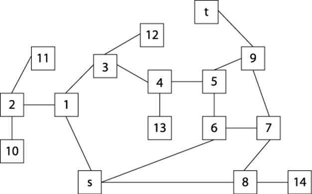
Figure 6-6. Graph representation of maze from Figure 6-5

To solve the maze, we need only find a path in the graph G=(V, E) of Figure 6-5 from the start vertex, s, to the target vertex, t. In this example, all edges are undirected, but one could easily consider directed edges if the maze imposed such restrictions.

The heart of Depth-First Search is a recursive dfsVisit(u) operation, which visits a vertex u that previously has not been visited. dfsVisit(u) records its progress by coloring vertices one of three colors:

White

Vertex has not yet been visited

Gray

Vertex has been visited, but it may have an adjacent vertex that has not yet been visited

Black

Vertex has been visited and so have all of its adjacent vertices

DEPTH-FIRST SEARCH SUMMARY

Best, Average, Worst: O(V+E)

depthFirstSearch (G,s)

foreach v in V do

discovered[v] = finished[v] = pred[v] = -1

color[v] = White

counter = 0

dfsVisit(s)

end

dfsVisit(u)

color[u] = Gray

discovered[u] = ++counter

foreach neighbor v of u do

if color[v] = White then

pred[v] = u

dfsVisit(v)

color[u] = Black

finished[u] = ++counter

end

Initially all vertices are marked as not visited

Find unvisited neighbor and head in that direction

Once all neighbors are visited, this vertex is done

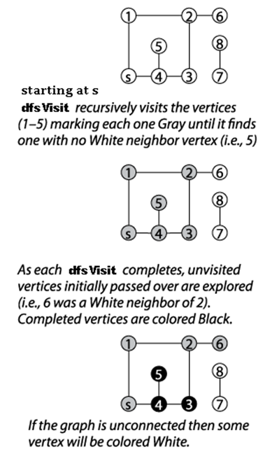
Figure 6-7. Depth-First Search example

Initially, each vertex is colored white to represent that it has not yet been visited, and Depth-First Search invokes dfsVisit on the source vertex, s. dfsVisit(u) colors u gray before recursively invoking dfsVisit on all adjacent vertices of u that have not yet been visited (i.e., they are colored white). Once these recursive calls have completed, u can be colored black, and the function returns. When the recursive dfsVisit function returns, Depth-First Search backtracks to an earlier vertex in the search (indeed, to a vertex that is colored gray), which may have an unvisited adjacent vertex that must be explored.

For both directed and undirected graphs, Depth-First Search investigates the graph from s until all vertices reachable from s are visited. During its execution, Depth-First Search traverses the edges of the graph, computing information that reveals the inherent, complex structure of the graph. Depth-First Search maintains a counter that is incremented when a vertex is first visited (and colored gray) and when Depth-First Search is done with the vertex (and it is colored black). For each vertex, Depth-First Search records:

pred[v]

The predecessor vertex that can be used to recover a path from the source vertex s to the vertex v

discovered[v]

The value of the incrementing counter when Depth-First Search first encounters vertex v

finished[v]

The value of the incrementing counter when Depth-First Search is finished with vertex v

The order in which vertices are visited will change the value of the counter, and so will the order in which the neighbors of a vertex are listed. This computed information is useful to a variety of algorithms built on Depth-First Search, including topological sort and identifying strongly connected components.

Given the graph in Figure 6-6 and assuming that the neighbors of a vertex are listed in increasing numerical order, the information computed during the search is shown in Figure 6-8. The coloring of the vertices of the graph shows the snapshot just after the fifth vertex (in this case vertex 13) is colored black. Some parts of the graph (i.e., the vertices colored black) have been fully searched and will not be revisited. Note that (a) white vertices have not been visited yet so their discovered[] values remain uncomputed; (b) black vertices have computed finished[] values since they have been fully processed; and (c) gray vertices have discovered[] values since they are currently being recursively visited by dfsVisit.

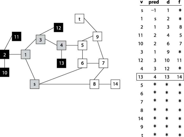
Figure 6-8. Computed pred, discovered (d), and finished (f) data for a sample undirected graph; snapshot taken after five vertices are colored black.

Depth-First Search has no global awareness of the graph, and so it will blindly search the vertices <5, 6, 7, 8>, even though these are in the wrong direction from the target, t. Once Depth-First Search completes, the pred[] values can be used to generate a path from the original source vertex, s, to each vertex in the graph.

Note that this path may not be the shortest possible path; when Depth-First Search completes, the path from s to t has seven vertices <s, 1, 3, 4, 5, 9, t>, while a shorter path of five vertices exists <s, 6, 5, 9, t>. Here the notion of a “shortest path” refers to the number of decision points between s and t.

Input/Output

The input is a graph G=(V, E) and a source vertex s ∈ V representing the start location.

Depth-First Search produces three computed arrays. discovered[v] records the depth-first numbering of the counter when v is first visited; it is the value of the counter when dfsVisit is invoked. pred[v] records the predecessor vertex of v based on the depth-first search ordering.finished[v] records the depth-first numbering of the counter when v has been completely visited; it is the value of the counter when control returns from dfsVisit.

Context

Depth-First Search only needs to store a color (either white, gray, or black) with each vertex as it traverses the graph. Thus Depth-First Search requires only O(n) overhead in storing information while it explores the graph starting from s.

Depth-First Search can store its processing information in arrays separately from the graph. Indeed, the only requirements Depth-First Search has on the graph is that one can iterate over the vertices that are adjacent to a given vertex. This feature makes it easy to perform Depth-First Search on complex information, since the dfsVisit function accesses the original graph as a read-only structure.

Solution

Example 6-1 contains a sample C++ solution. Note that vertex color information is used only within the dfsVisit methods.

Example 6-1. Depth-First Search implementation

#include "dfs.h"

// visit a vertex, u, in the graph and update information

void dfsVisit (Graph const &graph, int u, /* in */

vector<int> &discovered, vector<int> &finished, /* out */

vector<int> &pred, vector<vertexColor> &color, /* out */

int &ctr, list<EdgeLabel> &labels) { /* out */

color[u] = Gray;

discovered[u] = ++ctr;

// process all neighbors of u.

for (VertexList::const_iterator ci = graph.begin(u);

ci != graph.end(u); ++ci) {

int v = ci->first;

// Compute edgeType and add to labelings. Default to cross

edgeType type = Cross;

if (color[v] == White) { type = Tree; }

else if (color[v] == Gray) { type = Backward; }

else { if (discovered[u] < discovered[v]) type = Forward; }

labels.push_back(EdgeLabel (u, v, type));

// Explore unvisited vertices immediately and record pred[].

// Once recursive call ends, backtrack to adjacent vertices.

if (color[v] == White) {

pred[v] = u;

dfsVisit (graph, v, discovered, finished, pred, color,

ctr, labels);

}

}

color[u] = Black; // our neighbors are complete; now so are we.

finished[u] = ++ctr;

}

/**

* Perform Depth-First Search starting from vertex s, and compute

* the values d[u] (when vertex u was first discovered), f[u] (when

* all vertices adjacent to u have been processed), pred[u] (the

* predecessor vertex to u in resulting depth-first search forest),

* and label edges according to their type.

*/

void dfsSearch (Graph const &graph, int s, /* in */

vector<int> &discovered, vector<int> &finished, /* out */

vector<int> &pred, list<EdgeLabel> &labels) /* out */

{

// initialize arrays and labels.

// Mark all vertices White to signify unvisited.

int ctr = 0;

const int n = graph.numVertices();

vector<vertexColor> color (n, White);

discovered.assign(n, −1);

finished.assign(n, −1);

pred.assign(n, −1);

labels.clear();

// Search starting at the source vertex.

dfsVisit (graph, s, discovered, finished, pred, color,

ctr, labels);

}

If the discovered[] and finished[] values are not needed, then the statements that compute these values (and the parameters to the functions) can be removed from the code solution in Example 6-1. Depth-First Search can capture additional information about the edges of the graph. Specifically, in the depth-first forest produced by Depth-First Search, there are four types of edges:

Tree edges

For all vertices v whose pred[v]=u, the edge (u, v) was used by dfsVisit(u) to explore the graph. These edges record the progress of Depth-First Search. Edge (s, 1) is an example in Figure 6-8.

Back edges

When dfsVisit(u) encounters a vertex v that is adjacent to u and is already colored gray, then Depth-First Search detects it is revisiting old ground. The edge (11, 2) is an example in Figure 6-8. That is, after reaching vertex 11, the algorithm checks neighbors to see where to go, but 2is gray, so it doesn’t expand search back in that direction.

Forward edges

When dfsVisit(u) encounters a vertex v that is adjacent to u and is already marked black, the edge (u, v) is a forward edge if vertex u was visited before v. Again, Depth-First Search detects it is revisiting old ground. The edge (s, 6) is an example in Figure 6-8. By the time the algorithm inspects this edge, it has already reached t and is now returning from recursive calls to the original vertex that launched the search; the edge (s, 8) is also a forward edge.

Cross edges

When dfsVisit(u) encounters a vertex v that is adjacent to u and is already marked black, the edge (u, v) is a cross edge if vertex v was visited before u. Cross edges are possible only in directed graphs.

The code to compute these edge labels is included in Example 6-1. For undirected graphs, the edge (u, v) may be labeled multiple times; it is common to accept the labeling the first time an edge is encountered, whether as (u, v) or as (v, u).

Analysis

The recursive dfsVisit function is called once for each vertex in the graph. Within dfsVisit, every neighboring vertex must be checked; for directed graphs, each edge is traversed once, whereas in undirected graphs they are traversed once and are seen one other time. In any event, the total performance cost is O(V+E).

Variations

If the original graph is unconnected, then there may be no path between s and some vertices; these vertices will remain unvisited. Some variations ensure that all vertices are processed by conducting additional dfsVisit executions on the unvisited vertices in the dfsSearch method. If this is done, pred[] values record a depth-first forest of depth-first tree search results. To find the roots of the trees in this forest, scan pred[] to find vertices r whose pred[r] value is −1.

Breadth-First Search

Breadth-First Search takes a different approach from Depth-First Search when searching a graph. Breadth-First Search systematically visits all vertices in the graph G=(V, E) that are k edges away from the source vertex s before visiting any vertex that is k+1 edges away. This process repeats until no more vertices are reachable from s. Breadth-First Search does not visit vertices in G that are not reachable from s. The algorithm works for undirected as well as directed graphs.

BREADTH-FIRST SEARCH SUMMARY

Best, Average, Worst: O(V+E)

breadthFirstSearch (G, s)

foreach v in V do

pred[v] = -1

dist[v] = ∞

color[v] = White

color[s] = Gray

dist[s] = 0

Q = empty Queue

enqueue (Q, s)

while Q is notempty do

u = head(Q)

foreach neighbor v of u do

if color[v] = White then

dist[v] = dist[u] + 1

pred[v] = u

color[v] = Gray

enqueue (Q, v)

dequeue (Q)

color[u] = Black

end

Initially all vertices are marked as not visited

Queue maintains collection of gray nodes that are visited

Once all neighbors are visited, this vertex is done

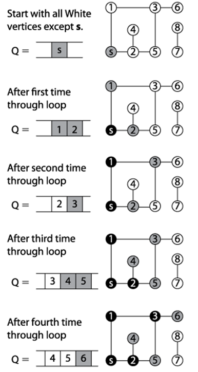
Figure 6-9. Breadth-First Search example

Breadth-First Search makes its progress without requiring any backtracking. It records its progress by coloring vertices white, gray, or black, as Depth-First Search did. Indeed, the same colors and definitions apply. To compare directly with Depth-First Search, we can take a snapshot ofBreadth-First Search executing on the same graph used earlier in Figure 6-6 after it colors its fifth vertex black (vertex 2) as shown in Figure 6-10. At the point shown in the figure, the search has colored black the source vertex s, vertices that are one edge away from s (1, 6, and 8), and vertex 2 which is two edges away from s.

The remaining vertices two edges away from s— { 3, 5, 7, 14 }— are all in the queue Q waiting to be processed. Some vertices three edges away from s have been visited—vertices {10,11}. Note that all vertices within the queue are colored gray, reflecting their active status.

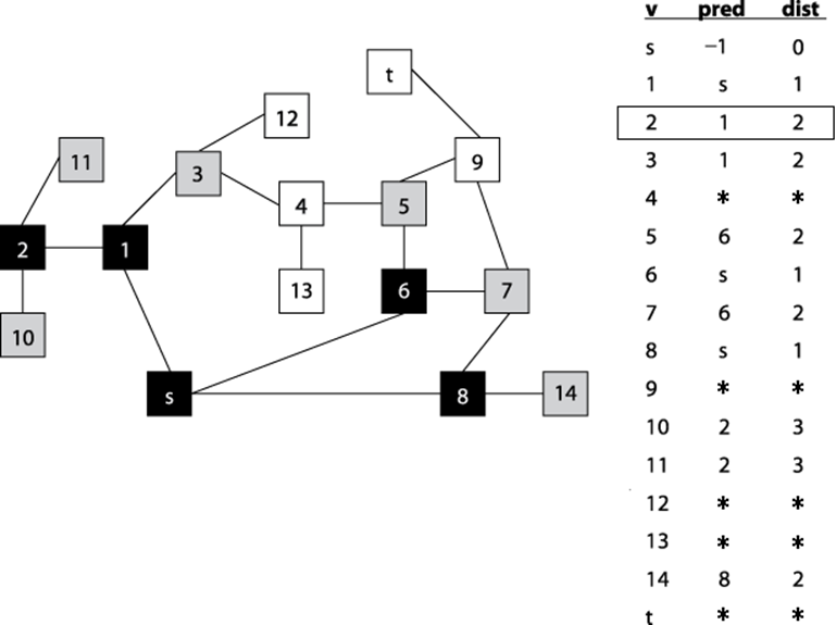
Figure 6-10. Breadth-First Search progress on graph after five vertices are colored black

Input/Output

The input is a graph G=(v, E) and a source vertex s ∈ V representing the start location.

Breadth-First Search produces two computed arrays. dist[v] records the number of edges in a shortest path from s to v. pred[v] records the predecessor vertex of v based on the breadth-first search ordering. The pred[] values encode the breadth-first tree search result; if the original graph is unconnected, then all vertices w unreachable from s have a pred[w] value of −1.

Context

Breadth-First Search stores the vertices being processed in a queue, thus there is O(V) storage. Breadth-First Search is guaranteed to find a shortest path in graphs whose vertices are generated “on the fly” (as will be seen in Chapter 7). Indeed, all paths in the generated breadth-first tree are shortest paths from s in terms of edge count.

Solution

A sample C++ solution is shown in Example 6-2. Breadth-First Search stores its state in a queue, and therefore there are no recursive function calls.

Example 6-2. Breadth-First Search implementation

#include "bfs.h"

/**

* Perform breadth-first search on graph from vertex s, and compute BFS

* distance and pred vertex for all vertices in the graph.

*/

void bfs_search (Graph const &graph, int s, /* in */

vector<int> &dist, vector<int> &pred) /* out */

{

// initialize dist and pred to mark vertices as unvisited. Begin at s

// and mark as Gray since we haven't yet visited its neighbors.

const int n = graph.numVertices();

pred.assign(n, −1);

dist.assign(n, numeric_limits<int>::max());

vector<vertexColor> color (n, White);

dist[s] = 0;

color[s] = Gray;

queue<int> q;

q.push(s);

while (!q.empty()) {

int u = q.front();

// Explore neighbors of u to expand the search horizon

for (VertexList::const_iterator ci = graph.begin(u);

ci != graph.end(u); ++ci) {

int v = ci->first;

if (color[v] == White) {

dist[v] = dist[u]+1;

pred[v] = u;

color[v] = Gray;

q.push(v);

}

}

q.pop();

color[u] = Black;

}

}

Analysis

During initialization, Breadth-First Search updates information for all vertices, with performance of O(V). When a vertex is first visited (and colored gray), it is inserted into the queue, and no vertex is added twice. Since the queue can add and remove elements in constant time, the cost of managing the queue is O(V). Finally, each vertex is dequeued exactly once and its adjacent vertices are traversed exactly once. The sum total of the edge loops, therefore, is bounded by the total number of edges, or O(E). Thus the total performance is O(V+E).

Single-Source Shortest Path

Suppose you want to fly a private plane on the shortest path from Saint Johnsbury, VT to Waco, TX. Assume you know the distances between the airports for all pairs of cities and towns that are reachable from each other in one nonstop flight of your plane. The best-known algorithm to solve this problem, Dijkstra’s Algorithm finds the shortest path from Saint Johnsbury to all other airports, although the search may be halted once the shortest path to Waco is known. A variation of this search (A*Search, discussed in Chapter 7), directs the search with heuristic information when approximate answers are acceptable.

In this example, we minimize the distance traversed. In other applications we might replace distance with time (e.g., deliver a packet over a network as quickly as possible) or with cost (e.g., find the cheapest way to fly from St. Johnsbury to Waco). Solutions to these problems also correspond to shortest paths.

Dijkstra’s Algorithm relies on a data structure known as a priority queue (PQ). A PQ maintains a collection of items, each of which has an associated integer priority that represents the importance of an item. A PQ allows one to insert an item, x, with its associated priority, p. Lower values of p represent items of higher importance. The fundamental operation of a PQ is getMin which returns the item in PQ whose priority value is lowest (or in other words, is the most important item). Another operation, decreasePriority may be provided by a PQ which allows one to locate a specific item in the PQ and reduce its associated priority value (which increases its importance) while leaving the item in the PQ.

DIJKSTRA’S ALGORITHM SUMMARY

Best, Average, Worst: O((V+E)*log V)

singleSourceShortest (G, s)

PQ = empty Priority Queue

foreach v in V do

dist[v] = ∞

pred[v] = -1

dist[s] = 0

foreach v in V do

insert (v, dist[v]) into PQ

while PQ is notempty do

u = getMin(PQ)

foreach neighbor v of u do

w = weight of edge (u, v)

newLen = dist[u] + w

if newLen < dist[v] then

decreasePriority (PQ, v, newLen)

dist[v] = newLen

pred[v] = u

end

Initially all vertices are considered to be unreachable

Populate PQ with vertices by shortest path distance

Remove vertex which has shortest distance to source

If discovered a shorter path from s to v record and update PQ

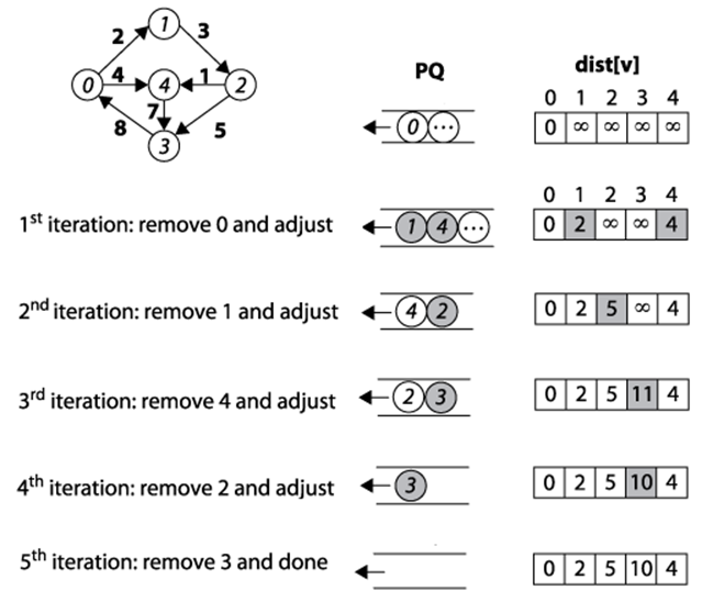
Figure 6-11. Dijkstra’s Algorithm example

Dijkstra’s Algorithm conceptually operates in greedy fashion by expanding a set of vertices, S, for which the shortest path from s to every vertex v ∈ S is known, but only using paths that include vertices in S. Initially, S equals the set {s}. To expand S, as shown in Figure 6-12, Dijkstra’s Algorithm finds the vertex v ∈ V-S (i.e., the vertices outside the shaded region in Figure 6-12) whose distance to s is smallest, and follows v’s edges to see whether a shorter path exists to another vertex. After processing v₂, for example, the algorithm determines that the distance from s to v₃containing only vertices in S is really 17 through the path <s, v₂, v₃>. Once S equals V, the algorithm completes.

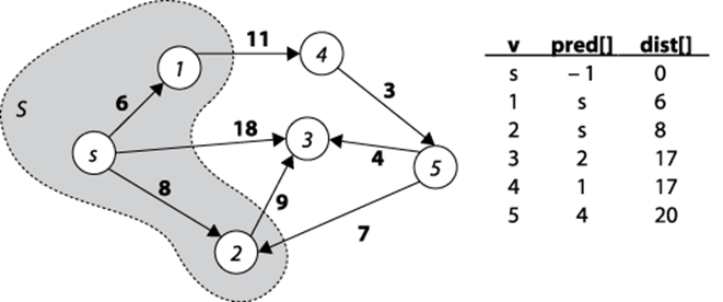
Figure 6-12. Dijkstra’s Algorithm expands the set S

Input/Output

A directed, weighted graph G=(V, E) and a source vertex s ∈ V. Each edge e=(u, v) has an associated positive weight in the graph.

Dijkstra’s Algorithm produces two computed arrays. The primary result is the array dist[] of values representing the distance from source vertex s to each vertex in the graph. The secondary result is the array pred[] that can be used to rediscover the actual shortest paths from vertex s to each vertex in the graph.

The edge weights are positive (i.e., greater than zero); if this assumption is not true, then dist[] may contain invalid results. Even worse, Dijkstra’s Algorithm will loop forever if a cycle exists whose sum of all weights is less than zero.

Solution

As Dijkstra’s Algorithm executes, dist[v] represents the maximum length of the shortest path found from the source s to v using only vertices visited within the set S. Also, for each v ∈ S, dist[v] is correct. Fortunately, Dijkstra’s Algorithm does not need to create and maintain the setS. It initially constructs a set containing the vertices in V, and then it removes vertices one at a time from the set to compute proper dist[v] values; for convenience, we continue to refer to this ever-shrinking set as V-S. Dijkstra’s Algorithm terminates when all vertices are either visited or are shown to not be reachable from the source vertex s.

In the C++ solution shown in Example 6-3, a binary heap stores the vertices in the set V-S as a priority queue because, in constant time, one can locate the vertex with smallest priority (where the priority is determined by the vertex’s distance from s). Additionally, when a shorter path from s tov is found, dist[v] is decreased, requiring the heap to be modified. Fortunately, the decreasePriority operation (in a binary heap, it is known as decreaseKey) can be performed on average in O(log q) time, where q is the number of vertices in the binary heap, which will always be less than or equal to the number of vertices, V.

Example 6-3. Dijkstra’s Algorithm implementation

#include "BinaryHeap.h"

#include "Graph.h"

/** Given directed, weighted graph, compute shortest distance to

* vertices and record predecessor links for all vertices. */

void singleSourceShortest(Graph const &g, int s, /* in */

vector<int> &dist, /* out */

vector<int> &pred) { /* out */

// initialize dist[] and pred[] arrays. Start with vertex s by

// setting dist[] to 0. Priority Queue PQ contains all v in G.

const int n = g.numVertices();

pred.assign(n, −1);

dist.assign(n, numeric_limits<int>::max());

dist[s] = 0;

BinaryHeap pq(n);

for (int u = 0; u < n; u++) { pq.insert (u, dist[u]); }

// find vertex in ever-shrinking set, V-S, whose dist[] is smallest.

// Recompute potential new paths to update all shortest paths

while (!pq.isEmpty()) {

int u = pq.smallest();

// For neighbors of u, see if newLen (best path from s->u + weight

// of edge u->v) is better than best path from s->v. If so, update

// in dist[v] and re-adjust binary heap accordingly. Compute in

// long to avoid overflow error.

for (VertexList::const_iterator ci = g.begin(u);

ci != g.end(u); ++ci) {

int v = ci->first;

long newLen = dist[u];

newLen += ci->second;

if (newLen < dist[v]) {

pq.decreaseKey (v, newLen);

dist[v] = newLen;

pred[v] = u;

}

}

}

}

Arithmetic error may occur if the sum of the individual edge weights exceeds numeric_limits<int>::max() (although individual values do not). To avoid this situation, compute newLen using a long data type.

Analysis

In the implementation of Dijkstra’s Algorithm in Example 6-3, the loop that constructs the initial priority queue performs the insert operation V times, resulting in performance O(V log V). In the remaining while loop, each edge is visited once, and thus decreaseKey is called no more than E times, which contributes O(E log V) time. Thus, the overall performance is O((V+E) log V).

Dijkstra’s Algorithm For Dense Graphs

The following pseudocode describes a version of Dijkstra’s Algorithm suitable for dense graphs represented using an adjacency matrix. The C++ implementation found in Example 6-4 is simpler by not using a binary heap. The efficiency of this version is determined by considering how fast the smallest dist[] value in V-S can be retrieved. The while loop is executed V times, since S grows one vertex at a time. Finding the smallest dist[u] in V-S inspects all V vertices. Note that each edge is inspected exactly once in the inner loop within the while loop. Thus, the total running time of this version is O (V² + E).

DIJKSTRA’S ALGORITHM FOR DENSE GRAPHS SUMMARY

Best, Average, Worst: O(V²+E)

singleSourceShortest (G, s)

foreach v in V do

dist[v] = ∞

pred[v] = -1

visited[v] = false

dist[s] = 0

while there exists unvisited vertex do

u = find dist[u] that is smallest of unvisited vertices

if dist[u] = ∞ then return

visited[u] = true

foreach neighbor v of u do

w = weight of edge (u, v)

newLen = dist[u] + w

if newLen < dist[v] then

dist[v] = newLen

pred[v] = u

end

Initially all vertices are considered to be unreachable

Stop when an unreachable vertex is found

Find vertex which has shortest distance to source

If discovered a shorter path from s to v record new length

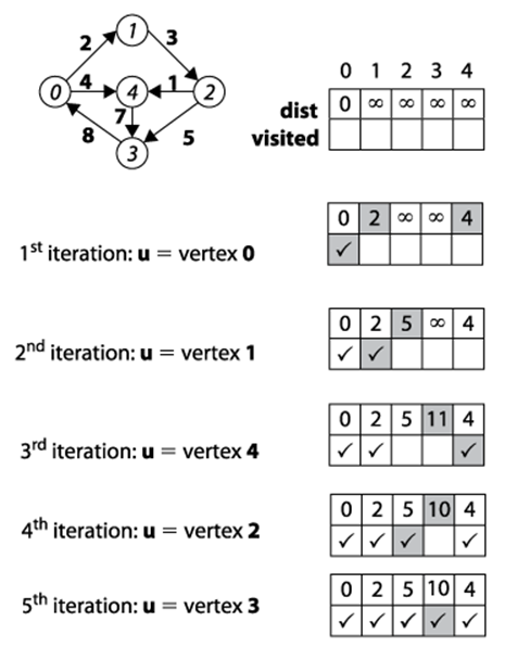
Figure 6-13. Dijkstra’s Algorithm Dense Graphs example

Example 6-3 is optimized to reduce the overhead of using C++ standard template library objects. This leads to impressive performance benefits.

Example 6-4. Optimized Dijkstra’s Algorithm for dense graphs

/**

* Given int[][] of edge weights in raw form, compute shortest

* distance to all vertices in graph (dist) and record predecessor

* links for all vertices (pred) to be able to recreate these

* paths. An edge weight of INF means no edge.

*/

void singleSourceShortestDense(int n, int ** const weight, int s, /* in */

int *dist, int *pred) { /* out */

// initialize dist[] and pred[] arrays. Start with vertex s by setting

// dist[] to 0. All vertices are unvisited.

bool *visited = new bool[n];

for (int v = 0; v < n; v++) {

dist[v] = numeric_limits<int>::max();

pred[v] = −1;

visited[v] = false;

}

dist[s] = 0;

// find shortest distance from s to unvisited vertices. Recompute

// potential new paths to update all shortest paths. Exit if u remains −1.

while (true) {

int u = −1;

int sd = numeric_limits<int>::max();

for (int i = 0; i < n; i++) {

if (!visited[i] && dist[i] < sd) {

sd = dist[i];

u = i;

}

}

if (u == −1) { break; }

// For neighbors of u, see if length of best path from s->u + weight

// of edge u->v is better than best path from s->v. Compute using longs.

visited[u] = true;

for (int v = 0; v < n; v++) {

int w = weight[u][v];

if (v == u) continue;

long newLen = dist[u];

newLen += w;

if (newLen < dist[v]) {

dist[v] = newLen;

pred[v] = u;

}

}

}

delete [] visited;

}

Variations

We may seek the most reliable path to send a message from one point to another through a network where we know the probability that any leg of a transmission delivers the message correctly. The probability of any path (sequence of legs) delivering a message correctly is the product of all the probabilities along the path. Using the same technique that made multiplication possible on a slide rule, we can replace the probability on each edge with minus the logarithm of the probability. The shortest path in this new graph corresponds to the most reliable path in the original graph.

Dijkstra’s Algorithm cannot be used when edge weights are negative. However, Bellman-Ford can be used as long as there is no cycle whose edge weights sum to a value less than zero. The concept of a “shortest path” is meaningless when such a cycle exists. Although the sample graph inFigure 6-11 contains a cycle involving vertices {1,3,2}, the edge weights are positive, so Bellman-Ford and Dijkstra’s Algorithm will work.

BELLMAN-FORD SUMMARY

Best, Average, Worst: O(V*E)

singleSourceShortest (G, s)

foreach v in V do

dist[v] = ∞

pred[v] = -1

dist[s] = 0

for i = 1 to n do

foreach edge (u,v) in E do

newLen = dist[u] + weight of edge (u,v)

if newLen < dist[v] then

if i = n then report "Negative Cycle"

dist[v] = newLen

pred[v] = u

end

Initially all vertices are considered to be unreachable

If discovered a shorter path from s to v record new length

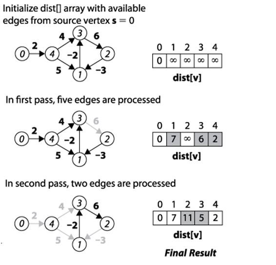
Figure 6-14. Bellman-Ford example

Example 6-5. Bellman-Ford algorithm for single source shortest path

#include "Graph.h"

/**

* Given directed, weighted graph, compute shortest distance to all vertices

* in graph (dist) and record predecessor links for all vertices (pred) to

* be able to recreate these paths. Graph weights can be negative so long

* as there are no negative cycles.

*/

void singleSourceShortest(Graph const &graph, int s, /* in */

vector<int> &dist, vector<int> &pred){ /* out */

// initialize dist[] and pred[] arrays.

const int n = graph.numVertices();

pred.assign(n, −1);

dist.assign(n, numeric_limits<int>::max());

dist[s] = 0;

// After n-1 times we can be guaranteed distances from s to all

// vertices are properly computed to be shortest. So on the nth

// pass, a change to any value guarantees there is negative cycle.

// Leave early if no changes are made.

for (int i = 1; i <= n; i++) {

bool failOnUpdate = (i == n);

bool leaveEarly = true;

// Process each vertex, u, and its respective edges to see if

// some edge (u,v) realizes a shorter distance from s->v by going

// through s->u->v. Use longs to prevent overflow.

for (int u = 0; u < n; u++) {

for (VertexList::const_iterator ci = graph.begin(u);

ci != graph.end(u); ++ci) {

int v = ci->first;

long newLen = dist[u];

newLen += ci->second;

if (newLen < dist[v]) {

if (failOnUpdate) { throw "Graph has negative cycle"; }

dist[v] = newLen;

pred[v] = u;

leaveEarly = false;

}

}

}

if (leaveEarly) { break; }

}

}

Intuitively Bellman-Ford operates by making n sweeps over a graph that check to see if any edge (u, v) is able to improve on the computation for dist[v] given dist[u] and the weight of the edge over (u, v). At least n−1 sweeps are needed, for example, in the extreme case that the shortest path from s to some vertex v goes through all vertices in the graph. Another reason to use n−1 sweeps is that the edges can be visited in an arbitrary order, and this ensures that all reduced paths have been found.

Bellman-Ford is thwarted only when there exists a negative cycle of directed edges whose total sum is less than zero. To detect such a negative cycle, we execute the primary processing loop n times (one more than necessary), and if there is an adjustment to some dist[] value, a negative cycle exists. The performance of Bellman-Ford is O(V*E), as clearly seen by the nested loops.

Comparing Single Source Shortest Path Options

The following summarizes the expected performance of the three algorithms by computing a rough cost estimate:

§ Bellman-Ford: O(V*E)

§ Dijkstra’s Algorithm for dense graphs: O(V²+E)

§ Dijkstra’s Algorithm with priority queue: O((V+E)*log V)

We compare these algorithms under different scenarios. Naturally, to select the one that best fits your data, you should benchmark the implementations as we have done. In the following tables, we execute the algorithms 10 times and discard the best and worst performing runs; the tables show the average of the remaining eight runs.

Benchmark data

It is difficult to generate random graphs. In Table 6-1, we show the performance on generated graphs with |V|=k²+2 vertices and |E|=k³-k²+2k edges in a highly stylized graph construction (for details, see the code implementation in the repository). Note that the number of edges is roughly n^1.5where n is the number of vertices in V. The best performance comes from using the priority queue implementation of Dijsktra’s Algorithm but Bellman-Ford is not far behind. Note how the variations optimized for dense graphs perform poorly.

Table 6-1. Time (in seconds) to compute single source shortest path on benchmark graphs

Dense graphs

For dense graphs, E is on the order of O(V²); for example, in a complete graph of n=|V| vertices that contains an edge for every pair of vertices, there are n(n−1)/2 edges. Using Bellman-Ford on such dense graphs is not recommended, since its performance degenerates to O(V³). The set of dense graphs reported in Table 6-2 is taken from a set of publicly available data sets used by researchers investigating the Traveling Salesman Problem (TSP)^[6^].We executed 100 trials and discarded the best and worst performances; the table contains the average of the remaining 98 trials. Although there is little difference between the priority queue and dense versions of Dijsktra’s Algorithm, there is a vast improvement in the optimized Dijsktra’s Algorithm, as shown in the fifth column of the table. In the final column we show the performance time for Bellman-Ford on the same problems, but these results are the averages of only five executions because the performance degrades so sharply. The lesson to draw from the last column is that the absolute performance of Bellman-Ford on sparse graphs seems to be quite reasonable, but when compared relatively to its peers on dense graphs, one sees clearly that it is the wrong algorithm to use.

Table 6-2. Time (in seconds) to compute single source shortest path on dense graphs

Sparse graphs

Large graphs are frequently sparse, and the results in Table 6-3 confirm that one should use the Dijsktra’s Algorithm with a priority queue rather than the implementation crafted for dense graphs; note how the implementation for dense graphs is 15 times slower. The rows in the table are sorted by the number of edges in the sparse graphs, since that appears to be the determining cost factor in the results.

Table 6-3. Time (in seconds) to compute single source shortest path on large sparse graphs

All Pairs Shortest Path

Instead of finding the shortest path from a single source, we often seek the shortest path between any two vertices (v_i, v_j); there may be several paths with the same total distance. The fastest solution to this problem uses the Dnamic Programming technique introduced in Chapter 3.

There are two interesting features of dynamic programming:

§ It solves small, constrained versions of the problem. When the constraints are tight, the function is simple to compute. The constraints are then systematically relaxed until finally the desired answer is computed.

§ Although one seeks an optimal answer to a problem, it is easier to compute the value of an optimal answer rather than the answer itself. In our case, we compute, for each pair of vertices (v_i, v_j), the length of a shortest path from v_i to v_j and perform additional computation to recover the actual path. In the pseudocode below, t, u, and v each represent a potential vertex of V.

Floyd-Warshall computes an n-by-n matrix dist such that for all pairs of vertices (v_i, v_j), dist[i][j] contains the length of a shortest path from v_i to v_j.

FLOYD-WARSHALL SUMMARY

Best, Average, Worst: O(V³)

allPairsShortestPath (G)

foreach u in V do

foreach v in V do

dist[u][v] = ∞

pred[u][v] = -1

dist[u][u] = 0

foreach neighbor v of u do

dist[u][v] = weight of edge (u,v)

pred[u][v] = u

foreach t in V do

foreach u in V do

foreach v in V do

newLen = dist[u][t] + dist[t][v]

if newLen < dist[u][v] then

dist[u][v] = newLen

pred[u][v] = pred[t][v]

end

Initially all vertices are considered to be unreachable

If discovered a shorter path from s to v record new length

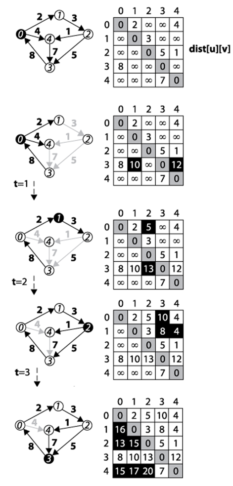
Figure 6-15. Floyd-Warshall example

Input/Output

A directed, weighted graph G=(V, E). Each edge e=(u, v) has an associated positive (i.e., greater than zero) weight in the graph.

Floyd-Warshall computes a matrix dist[][] representing the shortest distance from each vertex u to every vertex in the graph (including itself). Note that if dist[u][v] is ∞, then there is no path from u to v. The actual shortest path between any two vertices can be computed from a second matrix, pred[][], also computed by the algorithm.

Solution

A Dynamic Programming approach computes, in order, the results of simpler sub-problems. Consider the edges of G: these represent the length of the shortest path between any two vertices u and v that does not include any other vertex. Thus the dist[u][v] matrix is set initially to ∞ anddist[u][u] is set to zero (to confirm that there is no cost for the path from a vertex u to itself). Finally, dist[u][v] is set to the weight of every edge e=(u, v)∈E. At this point, the dist matrix contains the best computed shortest path (so far) for each pair of vertices, (u, v).

Now consider the next larger sub-problem, namely, computing the length of the shortest path between any two vertices u and v that might also include v₁. Dynamic Programming will check each pair of vertices (u, v) to check whether the path {u, v₁, v} has total distance smaller than the best score. In some cases, dist[u][v] is still ∞ because there was no information on any path between u and v. At other times, the sum of the paths from u to v₁ and then from v₁ to v is better than the current distance, and the algorithm records that total in dist[u][v]. The next larger sub-problem tries to compute length of shortest path between any two vertices u and v that might also include v₁ or v₂. Eventually the algorithm increases these sub-problems until the result is a dist[u][v] matrix that contains the shortest path between any two vertices u and v that might also include any vertex in the graph.

Floyd-Warshal computes the key optimization check whether dist[u][t] + dist[t][v] < dist[u][v]. Note that the algorithm also computes a pred[u][v] matrix which “remembers” that the newly computed shorted path from u to v must go through vertex t. The surprisingly brief solution is shown in Example 6-6.

Example 6-6. Floyd-Warshall algorithm for computing all pairs shortest path

#include "Graph.h"

void allPairsShortest(Graph const &graph, /* in */

vector< vector<int> > &dist, /* out */

vector< vector<int> > &pred) { /* out */

int n = graph.numVertices();

// Initialize dist[][] with 0 on diagonals, INFINITY where no edge

// exists, and the weight of edge (u,v) placed in dist[u][v]. pred

// initialized in corresponding way.

for (int u = 0; u < n; u++) {

dist[u].assign(n, numeric_limits<int>::max());

pred[u].assign(n, −1);

dist[u][u] = 0;

for (VertexList::const_iterator ci = graph.begin(u);

ci != graph.end(u); ++ci) {

int v = ci->first;

dist[u][v] = ci->second;

pred[u][v] = u;

}

}

for (int k = 0; k < n; k++) {

for (int i = 0; i < n; i++) {

if (dist[i][k] == numeric_limits<int>::max()) { continue; }

// If an edge is found to reduce distance, update dist[][].

// Compute using longs to avoid overflow of Infinity-distance.

for (int j = 0; j < n; j++) {

long newLen = dist[i][k];

newLen += dist[k][j];

if (newLen < dist[i][j]) {

dist[i][j] = newLen;

pred[i][j] = pred[k][j];}

}

}

}

}

The function shown in Example 6-7 constructs an actual shortest path (there may be more than one) from a given v_s to v_t. It works by recovering predecessor information from the pred matrix.

Example 6-7. Code to recover shortest path from computed pred[][]

/**

* Output path as list of vertices from s to t given the pred results

* from an allPairsShortest execution. Note that s and t must be valid

* integer vertex identifiers. If no path is found between s and t, then

* an empty path is returned.

*/

void constructShortestPath(int s, int t, /* in */

vector< vector<int> > const &pred, /* in */

list<int> &path) { /* out */

path.clear();

if (t < 0 || t >= (int) pred.size() || s < 0 || s >= (int) pred.size()) {

return;

}

// construct path until we hit source 's' or −1 if there is no path.

path.push_front(t);

while (t != s) {

t = pred[s][t];

if (t == −1) { path.clear(); return; }

path.push_front(t);

}

}

Analysis

The time taken by Floyd-Warshall is dictated by the number of times the minimization function is computed, which is O(V³), as can be seen from the three nested loops. The constructShortestPath function in Example 6-7 executes in O(E) since the shortest path might include every edge in the graph.

Minimum Spanning Tree Algorithms

Given an undirected, connected graph G=(V, E), one might be concerned with finding a subset ST of edges from E that “span” the graph because it connects all vertices. If we further require that the total weights of the edges in ST is the minimal across all possible spanning trees, then we are interested in finding a minimum spanning tree (MST).

Prim’s Algorithm shows how to construct an MST from such a graph by using a Greedy approach in which each step of the algorithm makes forward progress toward a solution without reversing earlier decisions. Prim’s Algorithm grows a spanning tree T one edge at a time until an MST results (and the resulting spanning tree is provably minimum). It randomly selects a start vertex s ∈ v to belong to a growing set S, and it ensures that T forms a tree of edges rooted at s. Prim’s Algorithm is greedy in that it incrementally adds edges to T until an MST is computed. The intuition behind the algorithm is that the edge (u, v) with lowest weight between u ∈ S and v ∈ V-S must belong to the MST. When such an edge (u, v) with lowest weight is found, it is added to T and the vertex v is added to S.

The algorithm uses a priority queue to store the vertices v ∈ V-S with an associated priority key equal to the lowest weight of some edge (u, v) where u ∈ S. This key value reflects the priority of the element within the priority queue; smaller values are of higher importance.

PRIM’S ALGORITHM SUMMARY

Best,Average,Worst: O((V+E)*log V)

computeMST (G)

foreach v∈V do

key[v] = ∞

pred[v] = -1

key[0] = 0

PQ = empty Priority Queue

foreach v in V do

insert (v, key[v]) into PQ

while PQ is notempty do

u = getMin(PQ)

foreach edge(u,v)∈E do

if PQ contains v then

w = weight of edge (u,v)

if w < key[v] then

pred[v] = u

key[v] = w

decreasePriority (PQ, v, w)

end

Initially all vertices are considered to be unreachable

Find vertex with lowest edge weight to computed MST

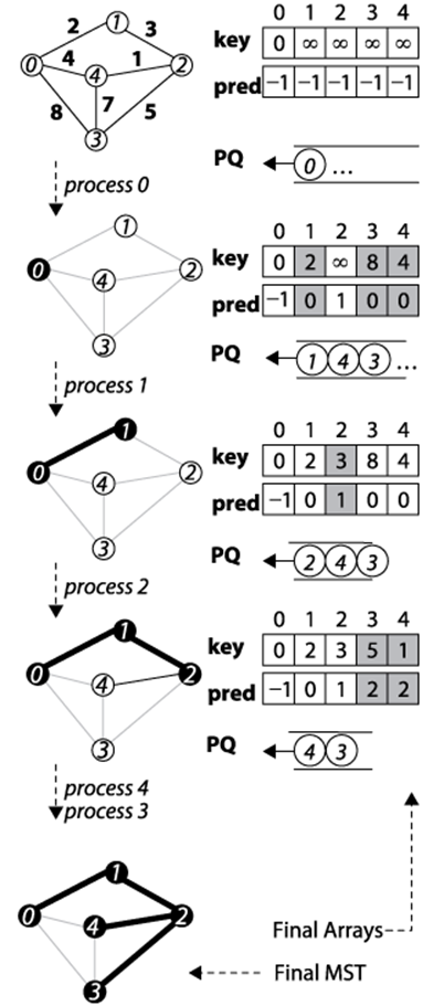
Figure 6-16. Prim’s Algorithm Example

Solution

The C++ solution shown in Example 6-8 relies on a binary heap to provide the implementation of the priority queue that is central to Prim’s Algorithm. Ordinarily, using a binary heap would be inefficient because of the check in the main loop for whether a particular vertex is a member of the priority queue (an operation not supported by binary heaps). However, the algorithm ensures that each vertex is removed from the priority queue only after being processed by the program, thus it maintains a status array inQueue[] that is updated whenever a vertex is extracted from the priority queue. In another implementation optimization, it maintains an external array key[] recording the current priority key for each vertex in the queue, which again eliminates the need to search the priority queue for a given vertex.

Prim’s Algorithm randomly selects one of the vertices to be the starting vertex, s. When the minimum vertex, u, is removed from the priority queue PQ and “added” to the visited set S, the algorithm uses existing edges between S and the growing spanning tree T to reorder the elements in PQ. Recall that the decreasePriority operation moves an element closer to the front of PQ.

Example 6-8. Prim’s Algorithm implementation with binary heap

/**

* Given undirected graph, compute MST starting from a randomly

* selected vertex. Encoding of MST is done using 'pred' entries.

*/

void mst_prim (Graph const &graph, vector<int> &pred) {

// initialize pred[] and key[] arrays. Start with arbitrary

// vertex s=0. Priority Queue PQ contains all v in G.

const int n = graph.numVertices();

pred.assign(n, −1);

vector<int> key(n, numeric_limits<int>::max());

key[0] = 0;

BinaryHeap pq(n);

vector<bool> inQueue(n, true);

for (int v = 0; v < n; v++) {

pq.insert(v, key[v]);

}

while (!pq.isEmpty()) {

int u = pq.smallest();

inQueue[u] = false;

// Process all neighbors of u to find if any edge beats best distance

for (VertexList::const_iterator ci = graph.begin(u);

ci != graph.end(u); ++ci) {

int v = ci->first;

if (inQueue[v]) {

int w = ci->second;

if (w < key[v]) {

pred[v] = u;

key[v] = w;

pq.decreaseKey(v, w);

}

}

}

}

}

Analysis

The initialization phase of Prim’s Algorithm inserts each vertex into the priority queue (implemented by a binary heap) for a total cost of O(V log V). The decreaseKey operation in Prim’s Algorithm requires O(log q) performance, where q is the number of elements in the queue, which will always be less than |V|. It can be called at most 2*|E| times since each vertex is removed once from the priority queue and each undirected edge in the graph is visited exactly twice. Thus the total performance is O((V+2*E)*log V) or O((V+E)*log V).

Variations

Kruskal’s Algorithm is an alternative to Prim’s Algorithm. It uses a “disjoint-set” data structure to build up the minimum spanning tree by processing all edges in the graph in order of weight, starting with the edge with smallest weight and ending with the edge with largest weight.Kruskal’s Algorithm can be implemented in O(E log E); with a sophisticated implementation of the disjoint-set data structure, this can be reduced to O(E log V). Details on this algorithm can be found in (Cormen et al., 2009).

Final Thoughts on Graphs

Storage Issues

When using a two-dimensional matrix to represent potential relationships among n elements in a set, the matrix requires n² elements of storage, yet there are times when the number of relationships is much smaller. In these cases—known as sparse graphs—it may be impossible to store large graphs with more than several thousand vertices because of the limitations of computer memory. Additionally, traversing through large matrices to locate the few edges in sparse graphs becomes costly, and this storage representation prevents efficient algorithms from achieving their true potential.

Each of these adjacency representations contains the same information. Suppose, however, you were writing a program to compute the cheapest flights between any pair of cities in the world that are served by commercial flights. The weight of an edge would correspond to the cost of the cheapest direct flight between that pair of cities (assuming that airlines do not provide incentives by bundling flights). In 2012, Airports Council International (ACI) reported a total of 1,598 airports worldwide in 159 countries, resulting in a two-dimensional matrix with 2,553,604 entries. The question “how many of these entries has a value?” is dependent upon the number of direct flights. ACI reported 79 million “aircraft movements” in 2012, roughly translating to a daily average of 215,887 flights. Even if all of these flights represented an actual direct flight between two unique airports (clearly the number of direct flights will be much smaller), this means that the matrix is 92% empty—a good example of a sparse matrix!

Graph Analysis

When applying the algorithms in this chapter, the essential factor that determines whether to use an adjacency list or adjacency matrix is whether the graph is sparse. We compute the performance of each algorithm in terms of the number of vertices in the graph, |V|, and the number of edges in the graph, |E|. As is common in the literature on algorithms, we simplify the presentation of the formulas that represent best, average, and worst case by using V and E within the big-O notation. Thus O(V) means a computation requires a number of steps that is directly proportional to the number of vertices in the graph. However, the density of the edges in the graph will also be relevant. Thus O(E) for a sparse graph is on the order of O(V), whereas for a dense graph it is closer to O(V²).

As we will see, the performance of some algorithms depends on the structure of the graph; one variation might execute in O((V+E)*log V) time, while another executes in O(V²+E) time. Which one is more efficient? Table 6-4 shows that the answer depends on whether the graph G is sparse or dense. For sparse graphs, O((V+E)*log V) is more efficient, whereas for dense graphs O(V²+E) is more efficient. The table entry labeled “Break-even graph” identifies the type of graphs for which the expected performance is the same O(V²) for both sparse and dense graphs; in these graphs, the number of edges is on the order of O(V²/log v).

Table 6-4. Performance comparison of two algorithm variations

References

Cormen, Thomas H., Charles E. Leiserson, Ronald L. Rivest, and Clifford Stein. Introduction to Algorithms, Second Edition. McGraw-Hill, 2001.