Modern Cryptography: Applied Mathematics for Encryption and Informanion Security (2016)

PART I. Foundations

Chapter 5. Essential Algebra

In this chapter we will cover the following:

Groups, rings, and fields

Diophantine equations

Basic matrix algebra

Algorithms

The history of algebra

Certain aspects of algebra are very important to the cryptographic algorithms you will be exploring later in this book. Those of you with a solid background in mathematics might be wondering how I could cover such a broad topic in a single chapter. Those of you without a solid background in mathematics might be wondering if you can learn enough and grasp enough of the concepts to apply them to cryptography later on.

Let me address these questions before you continue reading. As I did with Chapter 4, in this chapter I’m going to focus only on the basic information you need to help you understand the cryptographic algorithms covered later. Certainly, each of these topics could be given much more coverage. Entire books have been written on abstract algebra, matrix mathematics, and algorithms—in fact, some rather large tomes have been written just on algorithms! But you don’t necessarily need all those details to understand what you will encounter in this book. I would, however, certainly recommend that you explore these topics in more depth at some point. In this chapter, as with the last, I won’t delve into mathematical proofs. This means that you must accept a few things simply on faith—or you can refer to numerous mathematical texts that do indeed provide proofs for these concepts.

Those of you with a less rigorous mathematical background should keep in mind that, although you’ll need to have a firm grasp of the concepts presented in this chapter, you don’t need to become a mathematician (though I would be absolutely delighted if this book motivated you to study mathematics more deeply). It might take a mathematician to create cryptographic algorithms, but anyone can understand the algorithms I’ll present here. The ultimate goal of this book is to help you understand existing cryptography. I will provide links to resources where you can get additional information and explanations if you need it.

Abstract Algebraic Structures

If you think of algebra only as solving linear and quadratic equations, as you probably did in secondary school, these first algebraic concepts might not seem like algebra at all. But solving such equations is only one application of algebra. A far more interesting topic, and one more pertinent to cryptography, is the study of sets and operations you can perform on those sets. This is the basis for abstract algebra. Mathematics students frequently struggle with these concepts, but I will endeavor to make them as simple as I can without leaving out any important details.

Special sets of numbers and the operations that can be accomplished on those numbers are important to abstract algebra, and groups, rings, and fields are simply sets of numbers with associated operations.

Let’s begin with some examples. Think about the set of real numbers, which is an infinite set, as you know. What operations can you do with numbers that are members of this set in which the result will still be within the set? You can add two real numbers, and the answer will always be a real number. You can multiply two real numbers, and the answer will always be a real number. What about the inverse of those two operations? You can subtract two real numbers and the answer will always be a real number. You can divide two real numbers and the answer will always be a real number (of course division by zero is undefined). At this point, you may think all of this is absurdly obvious, and you might even think it odd that I would spend a paragraph discussing it. However, let’s turn our attention to sets of numbers in which all of these facts are not true.

The set of all integers is an infinite set, just like the set of real numbers. You can add any two integers and the sum will be another integer. You can multiply any two integers and the product will be an integer. So far, this sounds just like the set of real numbers. So let’s turn our attention to the inverse operations. You can subtract any integer from another integer and the answer is an integer. But what about division? There are an infinite number of scenarios in which you cannot divide one integer by another to arrive at another integer. For example, dividing 6 by 2, 10 by 5, 21 by 3, or infinitely more examples, gives you an integer. But divide 5 by 2, or 20 by 3, and the answer is not an integer; instead, it’s a rational number. And there are infinitely more examples like this. Therefore, if I want to limit myself only to integers, I cannot use division as an operation.

Let’s continue with examples for a moment to help demonstrate these concepts. Imagine that you want to limit your mathematics to an artificial world in which only integers exist. (Set aside, for now, any considerations of why you might do this, and just focus on this thought experiment for a moment.) In this artificial world that you have created, the addition operation exists and functions as it always has, and so does the inverse of addition, subtraction. The multiplication operation behaves as you would expect. In this imaginary world, however, the division operation simply does not exist, because it has the very real possibility of producing non-integer answers, and such answers do not exist in our imaginary world of “only integers.”

And one last hypothetical situation should help clarify these basic points. What if you limit yourself to natural numbers, or counting numbers, only. You can add any two counting numbers and the answer will always be a natural number. You can also multiply any two natural numbers and rest assured that the product will be another natural number. You can also subtract some natural numbers and the answer will be a natural number—but there are infinitely many cases for which this is not true. For example, if you attempt to subtract 7 from 5, the answer is a negative number, which is not a natural number. In fact, any time you attempt to subtract a larger natural number from a smaller natural number, the result will not be a natural number. Furthermore, division is just as tricky with natural numbers as it is with integers. In an infinite number of cases, the answer will not be a natural number. In this imaginary world of only natural numbers, addition and multiplication work exactly as you would expect. But their inverse operations, subtraction and division, simply do not exist.

Abstract algebra concerns itself with structures just like this. These structures (groups, rings, fields, and so on) comprise a set of numbers and certain operations that can be performed on those numbers. The only operations allowed in a given structure are those whose result would fit within the prescribed set of numbers. You were introduced to similar concepts in Chapter 4, with modulo arithmetic, where the numbers used were integers bound by the modulo.

Don’t be overly concerned with the term abstract algebra. Some sources call it modern algebra—but since it dates back a few centuries, that may be a misnomer. Later in this book, when we discuss asymmetric cryptography—particularly in Chapter 11—you’ll see several practical applications. Even the symmetric algorithm, Advanced Encryption Standard (AES), which you will study in Chapter 7, applies some of these structures.

Groups

A group is an algebraic system consisting of a set, which includes an identity element, one operation, and its inverse operation. An identity element is a number within a set that, when combined with another number in some operation, leaves that number unchanged. Mathematically, the identity element I can be expressed as follows:

a * I = a

where * is any operation that you might specify—not necessarily multiplication.

With respect to the addition operation, 0 (zero) is the identity element. You can add 0 to any member of any given group, and you will still have 0. With respect to multiplication, 1 is the identity element. Any number multiplied by 1 is still the same number.

Every group must satisfy four properties: closure, associativity, identity, and invertibility:

Closure is the simplest of these properties. This was discussed a bit earlier in this chapter. Closure means that any operation performed on a member of the set will result in an answer that is also a member of the set.

Associativity means that you can rearrange the elements of a set of values in an operation without changing the outcome. For example (2 + 2) + 3 = 7. But if I change the order and instead write 2 + (2 + 3), the answer is still 7.

Identity was already discussed.

Invertibility simply means that a given operation on an element in a set can be inverted. Subtraction is the inversion of addition; division is the inversion of multiplication.

Think back to the example set of integers. Integers constitute a group. First there is an identity element, zero. There is also one operation (addition) and its inverse (subtraction). Furthermore you have closure. Any element of the group (that is, any integer) added to any other element of the group (any other integer) still produces a member of the group (in other words, the answer is still an integer).

Abelian Group

An abelian group, or commutative group, has an additional property called the commutative property: a + b = b + a if the operation is addition, and ab = ba if the operation is multiplication. The commutative requirement simply means that applying the group operation (whatever that operation might be) does not depend on the order of the group elements. In other words, whatever the group operation is, you can apply it to members of the group in any order you want.

To use a trivial example, consider the group of integers with the addition operation. Order does not matter:

4 + 2 = 2 + 4

Therefore, the set of integers with the operation of addition is an abelian group.

Tip

Obviously, division and subtraction operations could never be used for an abelian group, because the order of elements changes the outcome of the operation.

Cyclic Group

A cyclic group has elements that are all powers of one of its elements. So, for example, if you start with element x, then the members of a cyclic group would be

x^–2, x^–1, x⁰, x¹, x², x³, …

Of course, the other requirements for a group, as discussed previously, would still apply to a cyclic group. The basic element x is considered to be the generator of the group, since all other members of the group are derived from it. It is also referred to as a primitive element of the group. Integers could be considered a cyclic group, with 1 being the primitive element (the generator). All integers can be expressed as a power of 1 in this group. This may seem like a rather trivial example, but it is easy to understand.

Rings

A ring is an algebraic system consisting of a set, an identity element, two operations, and the inverse operation of the first operation. That is the formal definition of a ring, but it may seem a bit awkward at first read, so let’s examine this concept a bit further. If you think back to our previous examples, it should occur to you that when we are limited to two operations, they are usually addition and multiplication. And addition is the easiest to implement, with subtraction being the inverse.

A ring is essentially just an abelian group that has a second operation. We have seen that the set of integers with the addition operation form a group, and furthermore they form an abelian group. If you add the multiplication operation, the set of integers with both the addition and the multiplication operations form a ring.

Fields

A field is an algebraic system consisting of a set, an identity element for each operation, two operations, and their respective inverse operations. A field is like a group that has two operations rather than one, and it includes an inverse for both of those operations. It is also the case that every field is a ring, but not every ring will necessarily be a field. For example, the set of integers is a ring, but not a field (because the inverse of multiplication can produce answers that are not in the set of integers). Fields also allow for division (the inverse operation of multiplication), whereas groups do not.

A classic example is the field of rational numbers. Each number can be written as a ratio (a fraction) such as x/y (x and y could be any integers), and the additive inverse is simply –x/y. The multiplicative inverse is y/x.

Galois Fields

Galois fields are also known as finite fields. You will learn more about Évariste Galois himself in the “History Highlights” section of this chapter. These fields are very important in cryptography, and you will see them used in later chapters. They are called finite fields because they have a finite number of elements. If you think about some of the groups, rings, and fields we have discussed, you’ll realize they were infinite. The set of integers, rational numbers, and real numbers are all infinite. But Galois fields are finite.

In a Galois field, there are some integers such that n repeated terms equals zero. Put another way, there is some boundary on the field that makes it finite. The smallest n that satisfies this is a prime number referred to as the characteristic of the field. You will often see a Galois field defined as follows:

GF(pⁿ)

In this case, the GF does not denote a function. Instead, this statement is saying that there is a Galois field with p as the prime number (the characteristic mentioned previously), and the field has pⁿ elements. So a Galois field is some finite set of numbers (from 0 to pⁿ–1) and some mathematical operations (usually addition and multiplication) along with the inverses of those operations.

Now you may immediately be wondering, how can a finite field even exist? If the field is indeed finite, would it not be the case that addition and multiplication operations could lead to answers that don’t exist within the field? To understand how this works, think back to the modulus operation discussed in Chapter 4. Essentially, operations “wrap around” the modulus. If we consider the classic example of a clock, then any operation whose answer would be more than 12 simply wraps around. The same thing occurs in a Galois field: Any answer greater than pⁿ simply wraps around.

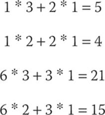
Let’s look at an example—another trivial example but it makes the point. Consider the Galois field GF(3¹). First, I hope you realize that 3¹ is the same as 3—most texts would simply write this as GF(3). So we have a Galois field defined by 3. In any case, addition or multiplication of the elements would exceed the number 3, so we simply wrap around. This example is easy to work with because it has only three elements: 1, 2, 3. Considering operations with those elements, several addition operations pose no problem at all:

1 + 1 = 2

1 + 2 = 3

However, others would be a problem,

2 + 2 = 4

except that we are working within a Galois field, which is similar to modulus operations, so 2 + 2 = 1 (we wrapped around at 3). Similarly, 2 + 3 = 2.

The same is true with multiplication (in both cases, we wrap around at 3):

2 × 2 = 1

2 × 3 = 0

In cryptography, we deal with Galois fields that are more complicated than this trivial example, but the principles are exactly the same.

Diophantine Equations

In a Diophantine equation, you are interested only in the integer solutions to the equation. Thus, a linear Diophantine equation is a linear equation ax + by = c with integer coefficients for which you are interested only in finding integer solutions.

There are two types of Diophantine equations: Linear Diophantine equations have elements that are of degree 1 or 0. Exponential Diophantine equations have at least one term that has an exponent greater than 1.

The word Diophantine comes from Diophantus of Alexandria, a third-century C.E. mathematician who studied such equations. You have actually seen Diophantine equations before, though you might not have realized it. The traditional Pythagorean theorem can be a Diophantine equation if you are interested in only integer solutions, which can be the case in many practical applications.

The simplest Diophantine equations are linear and are of this form,

ax + by = c

where a, b, and c are all integers. There is an integer solution to this problem, if and only if c is a multiple of the greatest common divisor of and b. For example, the Diophantine equation 3x + 6y = 18 does have solutions (in integers), since gcd(3,6) = 3, which does indeed evenly divide 18.

Matrix Math

A matrix is a rectangular arrangement, or array, of numbers in rows and columns. Rows run horizontally and columns run vertically. The dimensions of a matrix are stated m × n, where m is the number of rows and n is the number of columns. Here is an example:

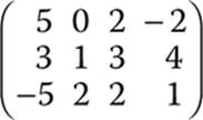
I will focus on 2 × 2 matrices for the examples in this section, but a matrix can be of any number of rows and columns, and it need not be a square. A vector can be considered a 1 × m matrix. In the preceding matrix example, you could have a vertical vector such as 5, 3, –5 or a horizontal vector such as 5, 0, 2, –2. A vector that is vertical is called a column vector, and one that is horizontal is called a row vector.

There are different types of matrices:

Column matrix A matrix with only one column

Row matrix A matrix with only one row

Square matrix A matrix that has the same number of rows and columns

Equal matrices Two matrices that have the same number of rows and columns (the same dimensions) and all their corresponding elements are exactly the same

Zero matrix A matrix that contains all zeros

Matrix Addition and Multiplication

If two matrices are of the same size, they can be added together by adding each element together. Consider the following example:

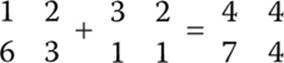
Start with the first row and first column in the first matrix (which is 1) and add that to the first row and the first column of the second matrix (which is 3); thus in the sum matrix, the first row and first column is 3 + 1 or 4. You repeat this for each cell.

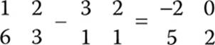
Subtraction works similarly:

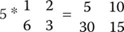
Multiplication, however, is a bit more complicated. Let’s take a look at an example multiplying a matrix by a scalar (a single number):

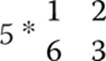
You simply multiply the scalar value by each element in the matrix:

Multiplication of two matrices is a bit more complex. You can multiply two matrices only if the number of columns in the first matrix is equal to the number of rows in the second matrix. You multiply each element in the first row of the first matrix by each element in the first column of the second matrix. Then you multiply each element of the second row of the first matrix by each element of the second column of the second matrix.

Let’s look at a conceptual example:

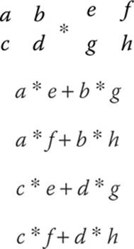
The product will be

Now if that is still not clear, we can examine a concrete example:

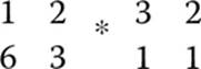
We begin with

The final answer is

This is why you can multiply two matrices only if the number of columns in the first matrix is equal to the number of rows in the second matrix.

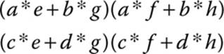
It is important that you remember that matrix multiplication, unlike traditional multiplication (with scalar values), is not commutative. Recall that the commutative property states a * b = b * a. If a and be are scalar values, then this is true; however, if they are matrices, this is not the case. For example, consider the matrix multiplication shown here.

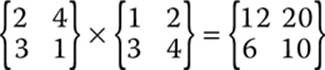
Now if we simply reverse the order, you can see that an entirely different answer is produced, as shown here.

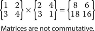
This example illustrates the rather important fact that matrix multiplication is not commutative.

Tip

If you need a bit more practice with matrix multiplication, try FreeMathHelp.com at www.freemathhelp.com/matrix-multiplication.html.

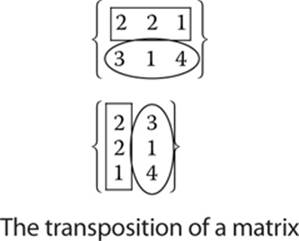
Matrix Transposition

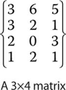
Matrix transposition simply reverses the order of rows and columns. Although we have focused on 2×2 matrices, the transposition operation is most easily seen with a matrix that has a different number of rows and columns. Consider the matrix shown next.

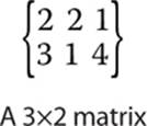
To transpose the matrix, the rows and columns are switched, creating a 2×3 matrix. The first row is now the first column. You can see this in the next illustration.

Submatrix

A submatrix is any portion of a matrix that remains after deleting any number of rows or columns. Consider the matrix shown here:

If you remove the second column and second row,

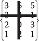
you are left with the matrix shown here:

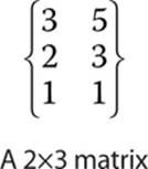
This matrix is a submatrix of the original matrix.

Identity Matrix

An identity matrix is actually rather simple. Think back to the identity property of groups. An identity matrix accomplishes the same goal, so that multiplying a matrix by its identity matrix leaves it unchanged. To create an identity matrix, you’ll need to have all the elements along the main diagonal set to 1 and the rest set to 0. Consider the matrix shown in Figure 5-1.

FIGURE 5-1 A 2×2 matrix

Now consider the identity matrix. It must have the same number of columns and rows, with its main diagonal set to all 1’s and the rest of the elements all 0’s. You can see the identity matrix in Figure 5-2.

FIGURE 5-2 The identity matrix

If you multiple the original matrix in Figure 5-3 by the identity matrix, the product will be the same as the original matrix. You can see this in Figure 5-3.

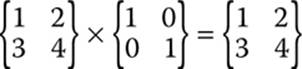
FIGURE 5-3 The product of a matrix and its identity matrix

Note

In these examples, I have focused not only on square, 2×2, matrices but also on matrices that consist of only integers. A matrix can consist of rational numbers, real numbers, or even functions. But since the goal was to provide an introduction to the concepts of matrix algebra, I have not delved into those nuances.

One application of matrix algebra is with linear transformations. A linear transformation, sometimes called a linear mapping or a linear function, is some mapping between two vector spaces that has the operations of addition and scalar multiplication.

Note

Wolfram MathWorld (http://mathworld.wolfram.com/VectorSpace.html) defines a vector space as follows: “A vector space V is a set that is closed under finite vector addition and scalar multiplication.” In other words, a vector space is a collection of objects (in our case, integers) called vectors, which may be added together and multiplied (“scaled”) by numbers called scalars.

Consider matrix multiplication (either with a scalar or with another matrix). That process maps each element in the first matrix to some element in the second matrix. This is a good example of a linear transformation. This process has many practical applications in physics, engineering, and cryptography.

Tip

For general tutorials on matrix algebra, the web site S.O.S. Mathematics offers a helpful set of tutorials at www.sosmath.com/matrix/matrix.html.

Algorithms

All the cryptography you will study from this point on consists of various algorithms. Those of you who have studied computer science have probably taken a course in data structures and algorithms. This section will introduce you to some concepts of algorithms and will then discuss general algorithm analysis in the context of sorting algorithms. At the conclusion of this section, we’ll study a very important algorithm.

Basic Algorithms

An algorithm is simply a systematic way of solving a problem. If you follow the procedure you get the desired results. Algorithms are a routine part of computer programming. Often the study of computer algorithms centers on sorting algorithms. The sorting of lists is a very common task and therefore a common topic in any study of algorithms.

It is also important that we have a clear method for analyzing the efficacy of a given algorithm. When considering any algorithm, if the desired outcome is achieved, then clearly the algorithm works. But the real question is, how well did it work? If you are sorting a list of 10 items, the time it takes to sort the list is not of particular concern. However, if your list has 1 million items, the time it takes to sort the list, and hence the algorithm you choose to perform the task, is of critical importance. Similar issues exist in evaluating modern cryptographic algorithms. It is obviously imperative that they work (that is, that they are secure), but they also have to work efficiently. For example, e-commerce would not be so widespread if the cryptographic algorithms used provided for an unacceptable lag.

Fortunately, there are well-defined methods for analyzing any algorithm. When analyzing algorithms we often consider the asymptotic upper and lower bounds. Asymptotic analysis is a process used to measure the performance of computer algorithms. This type of performance is based on a factor called computational complexity, which is usually a measure of either the time it takes or the resources (memory) needed for an algorithm to work. An algorithm can usually be optimized for time or for resources, but not both. The asymptotic upper bound is the worst-case scenario for the given algorithm, whereas the asymptotic lower bound is a best case.

Some analysts prefer to use an average case; however, knowing the best and worst cases can be useful in some situations. In simple terms, both the asymptotic upper and lower bounds must be within the parameters of the problem you are attempting to solve. You must assume that the worst-case scenario will occur in some situations.

The reason for this disparity between the asymptotic upper and lower bounds has to do with the initial state of a set. If you are applying a sorting algorithm to a set that is at its maximum information entropy (state of disorder), then the time it takes for the sorting algorithm to function will be the asymptotic upper bound. If, on the other hand, the set is very nearly sorted, then your algorithm may approach or achieve the asymptotic lower bound.

Perhaps the most common way to evaluate the efficacy of a given algorithm is the Big O notation. This method measures the execution of an algorithm, usually the number of iterations required, given the problem size n. In sorting algorithms, n is the number of items to be sorted. Stating some algorithm f(n) = O(g(n)) means it is less than some constant multiple of g(n). (The notation is read, “f of n is Big O of g of n.”) Saying an algorithm is 2n means that it will have to execute two times the number of items on the list. Big O notation essentially measures the asymptotic upper bound of a function, and it is also the most often used analysis.

Big O notation was first introduced by German mathematician Paul Bachmann in 1894 in his book Analytische Zahlentheorie, a work on analytic number theory. The notation was later popularized in the work of another German mathematician, Edmund Landau, and the notation is sometimes referred to as a “Landau symbol.”

Omega notation is the opposite of Big O notation. It is the asymptotic lower bound of an algorithm and gives the best-case scenario for that algorithm. It provides the minimum running time for an algorithm.

Theta notation combines Big O and Omega to provide the average case (average being arithmetic mean in this situation) for the algorithm. In our analysis, we will focus heavily on the Theta, also often referred to as the Big O running time. This average time gives a more realistic picture of how an algorithm executes.

Note

It can be confusing when a source refers to a “Big O running time” other than a Theta. I found several online sources that used “O notation,” when clearly what they were providing was actually . It is also possible that both could give the same answer.

Now that you have an idea of how the complexity and efficacy of an algorithm can be analyzed, let’s take a look at a few commonly studied sorting algorithms and apply these analytical tools.

Sorting Algorithms

Sorting algorithms are often used to introduce someone to the study of algorithms, because they are relatively easy to understand and they are so common. Because we have not yet explored modern cryptography algorithms, I will use sorting algorithms to illustrate concepts of algorithm analysis.

Elementary implementations of the merge sort sometimes use three arrays—one array for each half of the data set and one to store the final sorted list in. There are nonrecursive versions of the merge sort, but they don’t yield any significant performance enhancement over the recursive algorithm used on most machines. In fact, almost every implementation you will find of merge sort will be recursive, meaning that it simply calls itself repeatedly until the list is sorted.

The name derives from the fact that the lists are divided, sorted, and then merged, and this procedure is applied recursively. If you had an exceedingly large list and could separate the two sublists onto different processors, then the efficacy of the merge sort would be significantly improved.

Quick Sort

The quick sort is a very commonly used algorithm. Like the merge sort, it is recursive. Some books refer to the quick sort as a more effective version of the merge sort. In fact, the quick sort is the same as a merge sort (n ln n), but the difference is that the average case is also its best-case scenario (lower asymptotic bound). However, it has an O(n²), which indicates that its worst-case scenario is quite inefficient. For very large lists, the worst-case scenario may not be acceptable.

This recursive algorithm consists of three steps (which resemble those of the merge sort):

1. Choose an element in the array to serve as a pivot point.

2. Split the array into two parts. The split will occur at the pivot point. One array will include elements larger than the pivot and the other will include elements smaller than the pivot. One or the other should also include the pivot point.

3. Recursively repeat the algorithm for both halves of the original array.

One very interesting point is that the efficiency of the algorithm is significantly impacted by which element is chosen as the pivot point. The worst-case scenario of the quick sort occurs when the list is sorted and the leftmost element is chosen—this gives a complexity of O(n²). Randomly choosing a pivot point rather than using the leftmost element is recommended if the data to be sorted isn’t random. As long as the pivot point is chosen randomly, the quick sort has an algorithmic complexity of O(n log n).

Bubble Sort

The bubble sort is the oldest and simplest sort in use. By simple, I mean that from a programmatic point of view it is very easy to implement. Unfortunately, it’s also one of the slowest. It has a complexity of O(n²). This means that for very large lists, it is probably going to be too slow. As with most sort algorithms, its best case, or lower asymptotic bound, is O(n).

The bubble sort works by comparing each item in the list with the item next to it, and then swapping them if required. The algorithm repeats this process until it makes a pass all the way through the list without swapping any items (in other words, all items are in the correct order). This causes larger values to “bubble” to the end of the list while smaller values “sink” toward the beginning of the list, thus the name of the algorithm.

The bubble sort is generally considered to be the most inefficient sorting algorithm in common usage. Under best-case conditions (the list is already sorted), the bubble sort can approach a constant n level of complexity. General-case is an O(n²).

Even though it is one of the slower algorithms available, the bubble sort is used often simply because it is so easy to implement. Many programmers who lack a thorough enough understanding of algorithm efficiency and analysis depend on the bubble sort.

Now that we have looked at three common sorting algorithms, you should have a basic understanding of both algorithms and algorithm analysis. Next we will turn our attention to an important algorithm that is used in cryptography: the Euclidean algorithm.

Euclidean Algorithm

The Euclidean algorithm is a method for finding the greatest common divisor of two integers. That may sound like a rather trivial task, but with larger numbers that is not the case. It also happens that this algorithm plays a role in several cryptographic algorithms you will see later in this book. The Euclidean algorithm proceeds in a series of steps such that the output of each step is used as an input for the next one.

Here’s an example: Let k be an integer that counts the steps of the algorithm, starting with 0. Thus, the initial step corresponds to k = 0, the next step corresponds to k = 1, and then k = 2, k = 3, and so on. Each step after the first begins with two remainders, r_k–1 and r_k–2, from the preceding step. You will notice that at each step, the remainder is smaller than the remainder from the preceding step. So that r_k–1 is less than its predecessor r_k–2. This is intentional, and it is central to the functioning of the algorithm. The goal of the kth step is to find a quotient qk and remainder r_k such that the equation is satisfied:

r_k–2 = qk r_k–1 + r_k

where r_k < r_k–1. In other words, multiples of the smaller number r_k–1 are subtracted from the larger number r_k–2 until the remainder is smaller than r_k–1.

Let’s look at an example.

Let a = 2322, b = 654

2322 = 654·3 + 360 (360 is the remainder)

This tells us that the greatest common denominator of the two initial numbers, gcd(2322, 654), is equal to gcd(654, 360). These are still a bit unwieldy, so let’s proceed with the algorithm.

654 = 360·1 + 294 (the remainder is 294)

This tells us that gcd(654, 360) is equal to gcd(360, 294).

In the following steps, we continue this process until there is nowhere to go:

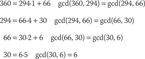
Therefore, gcd(2322,654) = 6.

This process is quite handy and can be used to find the greatest common divisor of any two numbers. And, as I previously stated, this will play a role in the cryptography you will study later in this book.

Tip

If you need a bit more on the Euclidean algorithm, there are some very helpful resources on the Internet. Rutgers University has a nice simple page on this issue, www.math.rutgers.edu/~greenfie/gs2004/euclid.html, as does the University of Colorado at Denver, www-math.ucdenver.edu/~wcherowi/courses/m5410/exeucalg.html.

Designing Algorithms

Designing an algorithm is a formal process that provides a systematic way of solving a problem. Therefore, it should be no surprise that there are systematic ways of designing algorithms. In this section we will examine a few of these methods.

The “divide-and-conquer” approach to algorithm design is a commonly used approach. In fact, it could be argued that it is the most commonly used approach. It works by recursively breaking down a problem into sub-problems of the same type until these sub-problems become simple enough to be solved directly. Once the sub-problems are solved, the solutions are combined to provide a solution to the original problem. In short, you keep subdividing the problem until you find manageable portions that you can solve, and after solving those smaller, more manageable portions, you combine those solutions to solve the original problem.

When you’re approaching difficult problems, such as the classic Tower of Hanoi puzzle, the divide-and-conquer method often offers the only workable way to find a solution. The divide-and-conquer method often leads to algorithms that are not only effective, but also efficient.

The efficiency of the divide-and-conquer method can be examined by considering the number of sub-problems being generated. If the work of splitting the problem and combining the partial solutions is proportional to the problem’s size n, then there are a finite number p of sub-problems of size ~ n/p at each stage. Furthermore, if the base cases require O (that is, constant-bounded) time, then the divide-and-conquer algorithm will have O(n log n) complexity. This is often used in sorting problems to reduce the complexity from O(n2). An O of n log n is fairly good for most sorting algorithms.

In addition to allowing you to devise efficient algorithms for solving complex problems, the divide-and-conquer approach is well suited for execution in multi-processor machines. The sub-problems can be assigned to different processors to allow each processor to work on a different sub-problem. This leads to sub-problems being solved simultaneously, thus increasing the overall efficacy of the process.

The second method is the greedy approach. The textbook An Introduction to Algorithms, by Thomas Cormen, Charles Leiserson, Ronald Rivest, and Clifford Stein (MIT Press, 2009), defines greedy algorithms as algorithms that select what appears to be the most optimal solution in a given situation. In other words, a solution is selected that is ideal for a specific situation, but it might not be the most effective solution for the broader class of problems. The greedy approach is used with optimization problems. To provide a precise description of the greedy paradigm, we must first consider a more detailed description of the environment in which most optimization problems occur. Most optimization problems include the following:

A collection of candidates—a set, a list, an array, or another data structure. How the collection is stored in memory is irrelevant.

A set of candidates that have previously been used.

A predicate solution that is used to test whether or not a given set of candidates provides an efficient solution. This does not check to determine whether those candidates provide an optimal solution, just whether or not they provide a working solution.

Another predicate solution (feasible) to test whether a set of candidates can be extended to a solution.

A selection function, which chooses some candidate that has not yet been used.

A function that assigns a value to a solution.

Essentially, an optimization problem involves finding a subset S from a collection of candidates C, where that subset satisfies some specified criteria. For example, the criteria may be “a solution such that the function is optimized by S.” Optimization may denote any number of factors, such as minimized or maximized. Greedy methods are distinguished by the fact that the selection function assigns a numerical value to each candidate C and chooses that candidate for which

SELECT( C ) is largest

or

SELECT( C ) is smallest

All greedy algorithms have this same general form. A greedy algorithm for a particular problem is specified by describing the predicates and the selection function. Consequently, greedy algorithms are often very easy to design for optimization problems.

The general form of a greedy algorithm is as follows:

functionselect (C : candidate_set) returncandidate;

functionsolution (S : candidate_set) returnboolean;

functionfeasible (S : candidate_set) returnboolean;

Tip

An Introduction to Algorithms is an excellent source for learning about algorithms. It is often used as a textbook in university courses. If you are looking for a thorough discussion of algorithms, I recommend this book.

P vs. NP

You have probably heard this issue bandied about quite a bit, even if you don’t have a rigorous mathematical background. It was even featured in an episode of the television drama Elementary. It involves a question that has significant implications for cryptography.

Many problems in mathematics are solvable via some polynomial equation, though not all problems are solvable in this fashion. Those that are not solvable are referred to as NP, or not polynomial (also known as nondeterministic polynomial time or not solvable in polynomial time). In complexity theory, NP-complete (NP-C) problems are the most difficult problems to solve because there are no polynomial equations for their solutions. That concept should be simple enough. P is polynomial, or more exactly, problems solvable in polynomial time. So what is the question that “P versus NP” addresses?

The question has to do with the fact that, to date, no one has proven that there is no polynomial solution for any NP-complete problem. If someone could provide a polynomial solution for any NP-complete problem, this would prove that all NP-complete problems do have a polynomial solution (in short, it would prove that there is no such thing as an NP-complete problem). In other words, as far as we know, there might be some polynomial time solution to these NP problems, but no one has proven that they cannot be solved in polynomial time.

Tip

When I say “proven” I mean provided with a mathematical proof.

There are essentially three classes of problems: P problems can be solved in polynomial time. NP problems cannot be solved in polynomial time, but they can be verified that a given solution is correct. NP-C problems simply cannot be addressed in any fashion in polynomial time.

One example of an NP-C problem is the subset sum problem, which can be summarized as follows: Given a finite set of integers, determine whether any non-empty subset of them sums to zero. A proposed answer is easy to verify for correctness; however, to date, no one has produced a faster way to solve the problem than simply to try each and every single possible subset. This is very inefficient.

At present, all known algorithms for NP-C problems require time that is super-polynomial in the input size. In other words, there is no polynomial solution for any NP-C problem. Therefore, to solve an NP-C problem, one of the following approaches is used:

Approximation An algorithm is used that quickly finds a suboptimal solution that is within a certain known range of the optimal one. In other words, an approximate solution is found.

Probabilistic An algorithm is used that provably yields good average runtime behavior for a given distribution of the problem instances.

Special cases An algorithm is used that is provably fast if the problem instances belong to a certain special case. In other words, an optimal solution is found only for certain cases of the problem.

Heuristic An algorithm that works well on many cases, but for which there is no proof that it is always fast. Heuristic methods are also considered rule-of-thumb.

We have examined NP-C problems in a general way, but now let’s look at a formal definition. A problem C is NP-C if

it is in NP

and

every other problem in NP is reducible to it.

In this instance, reducible means that for every problem L, there is a polynomial-time many-one reduction, a deterministic algorithm that transforms instances l ∈ L into instances c ∈ C, such that the answer to c is yes if and only if the answer to l is yes.

As a consequence of this definition, if you have a polynomial time algorithm for C, you could solve all problems in NP in polynomial time. This means that if someone ever finds a polynomial solution for any NP-C problem, then all problems have a solution, as I mentioned earlier.

In An Introduction to Algorithms, NP-C problems are illustrated by showing a problem that can be solved with a polynomial time algorithm, along with a related NP-C problem—for example, finding the shortest path is a polynomial time algorithm, whereas finding the longest path is an NP-C problem.

This formal definition was proposed by computer scientist Stephen Cook in 1971, who also showed that the Boolean satisfiability problem is NP-C.

Note

The details of the Boolean satisfiability problem are not really pertinent to our current discussion. If you are interested in more details, see the Association of Computing Machinery (ACM) paper on the topic: http://cacm.acm.org/magazines/2014/3/172516-boolean-satisfiability/fulltext.

Since Cook’s original results, thousands of other problems have been shown to be NP-C by reductions from other problems previously shown to be NP-C; many of these problems are collected in Michael Garey and David Johnson’s book Computers and Intractability: A Guide to the Theory of NP-Completeness (W.H. Freeman, 1979).

What does all of this have to do with cryptography? Actually quite a lot. As you will see in Chapters 10 and 11, modern public-key cryptography is based on mathematical problems that are very difficult to solve; these are NP problems (they cannot be solved in polynomial time). If someone were to prove that these NP problems actually had a polynomial time solution, that would seriously degrade the security of all modern public-key cryptography. As you will also see, public-key cryptography is critical to many modern technologies, including e-commerce.

Note

The P versus NP issue is a wonderful example of how mathematics that may seem abstract can have very real and practical implications.

History Highlights

In this section, I’ll provide a basic overview of some of the more important highlights in the history of algebra. The development of algebra progressed through three stages:

Rhetorical No use of symbols, verbal only

Syncopated Abbreviated words

Symbolic Use of symbols, used today

The rhetorical stage is so named because rather than use modern symbols, algebraic problems were described in words. As you might imagine, this was a serious impediment to the development of algebra. Consider for a moment your secondary school algebra courses, and imagine how difficult they would have been if you had to work without any symbols! The early Babylonian and Egyptian mathematicians used rhetorical algebra. The Greeks and Chinese did as well.

It was Diophantus, who you read about earlier in this chapter, who first used syncopated algebra in his book Arithmetica. Syncopated algebra used abbreviations rather than words.

Around 1500 C.E., symbols began to replace both syncopated and rhetorical algebra. By the 17th century, symbols were the primary way of performing mathematics. However, even then, the symbols used were not exactly the same as those you are most likely familiar with today.

Algebra is divided into two types:

Classical algebra Equation solving—the type of algebra you probably studied in secondary school. It is concerned with trying to find solutions to particular problems, such as quadratic equations.

Abstract/modern algebra Study of groups, or specialized sets of numbers and the operations on them—such as the groups, rings, and fields you read about earlier in this chapter.

The word algebra has an interesting origin. It was derived from the word jabr, an Arabic word used by mathematician Mohammed ibn-Mūsā al-Khwārizmī. In his book, The Compendious Book on Calculation by Completion and Balancing, written around the year 820 C.E., he used the word jabr to transpose subtracted terms to the other side of the equation—this is the cancelling you first encountered in secondary school. Eventually, the term al-jabr became algebra.

Our modern concepts of algebra evolved over many years—in fact, centuries—and has been influenced by many cultures.

Ancient Mediterranean Algebra

Ancient Egyptian mathematicians were primarily concerned with linear equations. One important document, the Rhind Papyrus (also known as the Ahmes Papyrus), written around 1650 B.C.E., appears to be a transcription of an even earlier work that documents ancient Egyptian mathematics. The Rhind Papyrus contains linear equations.

The Babylonians used rhetorical algebra and were already thinking about quadratic and cubic equations. This indicates that their mathematics were more advanced than that of the ancient Egyptians.

Ancient Greeks were most interested in geometric problems, and their approach to algebra reflects this. The “application of areas” was a method of solving equations using geometric algebra. It was described in Euclid’s Elements. Eventually the Greeks expanded even beyond that. In the book Introductio Arithmetica, by Nicomachus (60–120 C.E.), a method called the “bloom of Thymaridas” described a rule used for dealing with simultaneous linear equations. Greeks also studied number theory, beginning with Pythagoras and continuing with Euclid and Nicomachus.

As pivotal as the ancient Greek work in geometry was, their algebra had severe limitations. They did not recognize negative solutions, and such solutions were rejected. They did realize that irrational numbers existed, but they simply avoided them, considering them not to be numbers.

Ancient Chinese Algebra

At least as early as 300 B.C.E., the Chinese were also developing algebra. The book The Nine Chapters on the Mathematical Art comprised 246 problems. The book also dealt with solutions to linear equations, including solutions with negative numbers.

Ancient Arabic Algebra

Arab contributions to mathematics are numerous. Of particular note is Al-Karaji (c. 953–1029 C.E.), who has been described by some as the first person to adopt the algebra operations we are familiar with today. Al-Karaji was first to define the monomials x, x², x³, as well as the fractions thereof: 1/x, 1/x², 1/x³, and so on. He also presented rules for multiplying any two of these. Al-Karaji started a school of algebra that flourished for several hundred years.

Omar Khayyám (1048–1131 C.E.), another prominent Arab mathematician, poet, and astronomer, created a complete classification of cubic equations with geometric solutions found by means of intersecting conic sections. He also wrote that he hoped to give a full description of the algebraic solution of cubic equations in his book The Rubáiyát:

If the opportunity arises and I can succeed, I shall give all these fourteen forms with all their branches and cases, and how to distinguish whatever is possible or impossible so that a paper, containing elements which are greatly useful in this art, will be prepared.¹

Indian and other cultures’ mathematicians also significantly contributed to the study of algebra. In the western world, mathematics stagnated until the 12th century, when various translations of Arabic and Latin works became available in Europe, reigniting interest in mathematics.

Important Mathematicians

To give you a thorough understanding of the history of algebra, in this section, I will discuss a few of the more important mathematicians, providing you with a brief biographical sketch. Complete coverage of all relevant mathematicians would take several volumes.

Diophantus

You were briefly introduced to Diophantus, the third-century mathematician, when I discussed Diophantine equations. Diophantus was the first Greek mathematician to recognize fractions as numbers, and he introduced syncopated algebra. Unfortunately, little is known about his life.Interestingly, the following phrase was an algebra problem written rhetorically in the Greek Anthology (assembled around 500 C.E. by Metrodorus):

His boyhood lasted 1/6th of his life.

He married after 1/7th more.

His beard grew after 1/12th more.

And his son was born 5 years later.

The son lived to half his father’s age.

And the father died 4 years after the son.

The solution to this is that he married at the age of 26 and died at 84.

Tartaglia

Niccolo Tartaglia (c. 1499–1557) was an Italian mathematician and engineer. He applied mathematics to study how cannonballs are fired and what path they travel. Some consider him to be the father of ballistics. His first contribution to mathematics was a translation of Euclid’s Elements, published in 1543. This was the first-known translation of that work into any modern European language. He also published original works, most notably his book General Trattato di Numeri et Misure (General Treatise on Number and Measure) in 1556, which has been widely considered one of the best works on mathematics of the 16th century.

Tartaglia was known for his solutions to cubic equations. He shared his solutions with fellow mathematician Gerolamo Cardano, on the condition that Cardano keep them secret. However, many years later, Cardano published Tartaglia’s solution, giving Tartaglia full credit. (This, however, did not assuage Tartaglia’s anger.)

Descartes

René Descartes (1596–1650) may be better known for his work in philosophy, but he was also a mathematician who used symbolic algebra. He used lowercase letters from the end of the alphabet (x, y, z) to denote unknown values and lowercase letters from the beginning of the alphabet (a, b, c) for constants. The Cartesian coordinate system that most students learn in primary or secondary school was named after Descartes, and he is often called the “father of analytical geometry,” a combination of algebraic methods applied to geometry. His work also provided a foundation that was later applied by both Leibniz and Newton in the invention of calculus.

Galois

French mathematician Évariste Galois (1811–1932) made a number of important contributions to mathematics. Perhaps two of the most important, at least in reference to our current study of algebra, are his contributions to group theory (namely the Galois field, which we have discussed) and Galois theory. (The details of Galois theory are not necessary for our exploration of cryptography. However, it provided an important advancement in abstract algebra that involves both group theory and field theory.) Interestingly, in 1828, he tried to enter the École Polytechnique, a prestigious French mathematics institute, and failed the oral exam. So he entered the far less esteemed École Normale. A year later, he published his first paper on the topic of continued fractions.

Note

Popular conception views mathematicians as a rather quiet group, timidly working with formulas and proofs. Galois is one (of many) evidences that this perception is simply not true (or at least not always true). He had quite a colorful, and at times violent life. In 1831, Galois quit school to join an artillery unit of the military, which was later disbanded as several of the officers were accused of plotting to overthrow the government (they were later acquitted). Galois was known for rather vocal and extreme political protests, including proposing a toast to King Louis Philippe while holding a dagger above his cup. This was interpreted as a threat on the king’s life, and he was arrested but later acquitted. Galois was also arrested on Bastille Day while participating in a protest wearing the uniform of his disbanded artillery unit and carrying several weapons (a rifle, a dagger, and multiple pistols). He spent several months in jail for this incident. On May 30,1832, he was shot in a duel and later died of the wounds he suffered.

Conclusions

We explored several topics in this chapter, including groups, rings, and fields. These algebraic structures, particularly Galois fields, are very important to cryptography. Make certain you are familiar with them before proceeding to Chapter 6. Diophantine equations are so common in algebra that at least a basic familiarity of them is also important.

Next, we studied matrix algebra; matrices are not overly complex, as you read in the fundamentals explained in this chapter. You should be comfortable with matrices and the basic arithmetic operations on matrices, which are used in some cryptographic algorithms.

This chapter also introduced you to algorithms. An understanding of the sorting algorithms is not as critical as having a conceptual understanding of algorithms and algorithm analysis. Finally, you were introduced to some basics of the history of algebra. As with Chapters 3 and 4, the topics in this chapter are foundational and necessary for your understanding of subsequent chapters.

Note

Each of the topics presented in this chapter is the subject of entire books. This chapter provided a basic introduction—just enough information to help you understand the cryptography discussed later in this book. If you want to delve deeper into cryptography, you can study these various topics in the texts mentioned in this chapter as well as in other texts.

Test Your Knowledge

1. A __________________ is any equation for which you are interested only in the integer solutions to the equation.

2. A matrix that has all 1’s in its main diagonal and the rest of the elements are 0 is called what?

A. Inverse matrix

B. Diagonal matrix

C. Identity matrix

D. Reverse matrix

3. Omega notation is __________________.

A. the asymptotic upper bound of an algorithm

B. the asymptotic lower bound of an algorithm

C. the average performance of an algorithm

D. notation for the row and column of a matrix

4. A _________________ is an algebraic system consisting of a set, an identity element, two operations, and the inverse operation of the first operation.

A. ring

B. field

C. group

D. Galois field

5. A _________________ is an algebraic system consisting of a set, an identity element for each operation, two operations, and their respective inverse operations.

A. ring

B. field

C. group

D. Galois field

6. Yes or No: Is the set of integers a group with reference to multiplication?

7. Yes or No: Is the set of natural numbers a subgroup of the set of integers with reference to addition?

8. If a | b and a | c, then _________________.

9. A group that also has the commutative property is a __________________ group.

10. ___________________ is a process used to measure the performance of computer algorithms.

Answers

1. Diophantine equation

2. C

3. B

4. C

5. B

6. Yes

7. No

8. a | (b + c)

9. abelian

10. Asymptotic analysis

Endnote

1. From Omar Khayyám, The Rubáiyát of Omar Khayyám.