Applied Network Security Monitoring: Collection, Detection, and Analysis (2014)

SECTION 1. Collection

CHAPTER 3. The Sensor Platform

Abstract

This chapter introduces the most critical piece of hardware in an NSM deployment, the sensor. This includes a brief overview of the various NSM data types, and then discusses important considerations for purchasing and deploying sensors. Following, this chapter covers the placement of NSM sensors on the network, including a primer on creating network visibility maps for analyst use.

Keywords

Network Security Monitoring; Collection; Detection; Analysis; Intrusion Detection System; IDS; NIDS; Snort; Suricata; Security Onion; Packet; PCAP; Hardware; Data; Tap; Span; Placement; Diagram

The most important non-human component of NSM is the sensor. By definition, a sensor is a device that detects or measures a physical property and records, indicates, or otherwise responds to it. In the NSM world, a sensor is a combination of hardware and software used to perform collection, detection, and analysis. Within the NSM Cycle, a sensor might perform the following actions:

• Collection

• Collect PCAP

• Collect Netflow

• Generate PSTR Data from PCAP Data

• Generate Throughput Graphs from Netflow Data

• Detection

• Perform Signature-Based Detection

• Perform Anomaly-Based Detection

• Perform Reputation-Based Detection

• Use Canary Honeypots for Detection

• Detect Usage of Known-Bad PKI Credentials with a Custom Tool

• Detect PDF Files with Potentially Malicious Strings with a Custom Tool

• Analysis

• Provide Tools for Packet Analysis

• Provide Tools for Review of Snort Alerts

• Provide Tools for Netflow Analysis

Not every sensor performs all three functions of the NSM Cycle: however, the NSM sensor is the workhorse of the architecture and it is crucial that proper thought be put into how sensors are deployed and maintained. Having already stated how important collection is, it is necessary to respect that the sensor is the component that facilitates the collection. It doesn’t matter how much time you spend defining the threats to your network if you hastily throw together sensors without due process.

There are four primary architectural concerns when defining how sensors should operate on your network. These are the type of sensor being deployed, the physical architecture of the hardware being used, the operating system platform being used, and the placement of the sensor on the network. The tools installed on the sensor that will perform collection, detection, and analysis tasks are also of importance, but those will be discussed in extensive detail in subsequent chapters.

NSM Data Types

Later chapters of this book will be devoted entirely to different NSM data types, but in order to provide the appropriate context for discussing sensor architecture, it becomes pertinent to provide a brief overview of the primary NSM data types that are collected for detection and analysis.

Full Packet Capture (FPC) Data

FPC data provides a full accounting for every data packet transmitted between two endpoints. The most common form of FPC data is in the PCAP data format. While FPC data can be quite overwhelming due to its completeness, its high degree of granularity makes it very valuable for providing analytic context. Other data types, such as statistical data or packet string data, are often derived from FPC data.

Session Data

Session data is the summary of the communication between two network devices. Also known as a conversation or a flow, this summary data is one of the most flexible and useful forms of NSM data. While session data doesn’t provide the level of detail found in FPC data, its small size allows it to be retained for a much longer time, which is incredibly valuable when performing retrospective analysis.

Statistical Data

Statistical data is the organization, analysis, interpretation, and presentation of other types of data. This can take a lot of different forms, such as statistics supporting the examination of outliers from a standard deviation, or data points identifying positive or negative relationships between two entities over time.

Packet String (PSTR) Data

PSTR is derived from FPC data, and exists as an intermediate data form between FPC data and session data. This data format consists of clear text strings from specified protocol headers (for instance, HTTP header data). The result is a data type that provides granularity closer to that of FPC data, while maintaining a size that is much more manageable and allows increased data retention.

Log Data

Log data refers to raw log files generated from devices, systems, or applications. This can include items such as web-proxy logs, router firewall logs, VPN authentication logs, Windows security logs, and SYSLOG data. This data type varies in size and usefulness depending upon its source.

Alert Data

When a detection tool locates an anomaly within any of the data it is configured to examine, the notification it generates is referred to as alert data. This data typically contains a description of the alert, along with a pointer to the data that appears anomalous. Generally, alert data is incredibly small in size as it only contains pointers to other data. The analysis of NSM events is typically predicated on the generation of alert data.

When thinking about these data types holistically, its useful to be able to frame how their sizes compare. The largest data format is typically FPC data, followed by PSTR data, and then session data. Log, alert, and statistical data are generally miniscule compared to other data types, and can vary wildly based upon the types of data you are collecting and the sources you are utilizing.

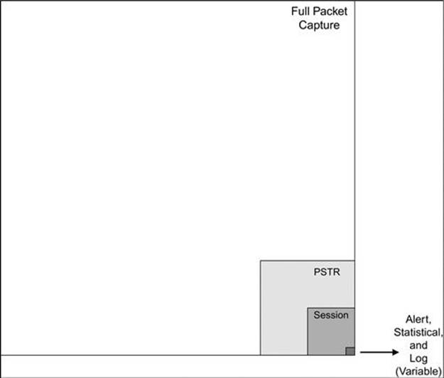
FIGURE 3.1 NSM Data Size Comparison

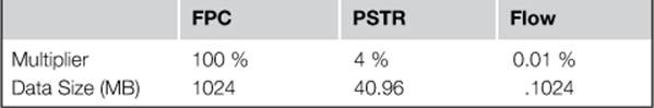
Quantifying these size differences can often be helpful, especially when attempting to determine sensor space requirements. This can vary drastically based upon the type of network environment. For instance, a user-heavy network might result in the generation of a lot more PSTR data than a server-heavy network segment. With that in mind, we have compiled the data from several different network types to generate some basic statistics regarding the size of particular data types given a static time period. Once again, log, alert, and statistical data are not included in this chart.

Caution

While the numbers shown in Table 3.1 provide a baseline of relative data sizes for the examples in this chapter, the relation between PSTR data, session data, and full packet capture data will vary wildly depending upon the types of network data you are capturing. Because of this, you should sample network traffic to determine the ratios that are accurate in your environment.

Table 3.1

NSM Data Size Comparison

Sensor Type

Depending on the size and threats faced by a network, sensors may have varying roles within the phases of the NSM Cycle.

Collection-Only

A collection-only sensor simply logs collected data such as FPC and session data to disk, and will sometimes generate other data (statistical and PSTR) based upon what has been collected. These are seen in larger organizations where detection tools access collected data remotely to perform their processing. Analysis is also done separately from the sensor, as relevant data is pulled to other devices as needed. A collection-only sensor is very barebones with no extra software installed, and analysts rarely have the ability to access it directly.

Half-Cycle

A half-cycle sensor performs all of the functions of a collection-only sensor, with the addition of performing detection tasks. For instance, a half-cycle sensor will log PCAP data to disk, but will also run a NIDS (such as Snort) either in real-time from the NIC or in near-real-time against PCAP data that is written to disk. When analysis must occur, data is pulled back to another device rather than the analysis being performed on the sensor itself. This is the most common type of sensor deployment, with analysts accessing the sensor directly on occasion to interact with various detection tools.

Full Cycle Detection

The last type of sensor is one in which collection, detection, and analysis are all performed on the sensor. This means that in addition to collection and detection tools, a full suite of analysis tools are installed on the sensor. This may include individual analysts profiles on the sensor, a graphical desktop environment, or the installation of a NIDS GUI such as Snorby. With a full cycle detection sensor, almost all NSM tasks are performed from the sensor. These types of sensors are most commonly seen in very small organizations where only a single sensor exists or where hardware resources are limited.

In most scenarios, a half cycle sensor is preferred. This is primarily due to the ease of implementing detection tools on the same system that data is collected. It is also much safer and more secure for analysts to pull copies of data back to dedicated analysis computers for their scrutiny ,rather than interacting with the raw data itself. This prevents mishandling of data, which may result in the loss of something important. Although analysts will need to interact with sensors at some level, they shouldn’t be using them as a desktop analysis environment unless there is no other option. The sensor must be protected as a network asset of incredible importance.

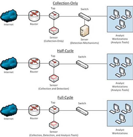
FIGURE 3.2 Sensor Types

Sensor Hardware

Once the proper planning has taken place, it becomes necessary to purchase sensor hardware. The most important thing to note here is that the sensor is, indeed, a server. This means that when deploying a sensor, server-grade hardware should be utilized. I’ve seen far too many instances where a sensor is thrown together from spare parts, or worse, I walk up to an equipment rack and see a workstation lying on its side being used as the sensor. This type of hardware is acceptable for a lab or testing scenario, but if you are taking NSM seriously, you should invest in reliable hardware.

A concerted engineering effort is required to determine the amount of hardware resources that will be needed. This effort must factor in the type of sensor being deployed, the amount of data being collected by the sensor, and the data retention desired.

We can examine the critical hardware components of the sensor individually. Before doing this, however, it helps to set up and configure a temporary sensor to help you determine your hardware requirements. This can be another server, a workstation, or even a laptop.

Prior to installing the temporary sensor, you should know where the sensor would be placed on the network. This includes the physical and logical placement that determines what network links the sensor will monitor. Determining sensor placement is discussed in depth later in this chapter.

Once the sensor has been placed on the network, you will utilize either a SPAN port or a network tap to get traffic to the device. Then you can install collection, detection, and analysis tools onto the sensor to determine the performance requirements of individual tools. Keep in mind that you don’t necessarily need a temporary sensor that is so beefy that it will handle all of those tools being enabled at once. Instead, you will want to enable the tools individually to calculate their performance load, and then total the results from all of the tools you will be utilizing to assess the overall need.

CPU

The amount of CPU resources required will mostly depend on the type of sensor being deployed. If you are deploying a collection-only sensor, then it is likely you will not need a significant amount of processing power, as these tasks aren’t incredibly processing intensive. The most CPU intensive process is typically detection, therefore, if you are deploying a half or full cycle sensor, you should plan for additional CPUs or cores. If you expect significant growth, then a blade chassis might be an enticing option, as it allows for the addition of more blades to increase CPU resources.

An easy way to begin planning for your sensor deployment is to map the number of cores required on the system to the tools being deployed. The specific requirements will vary greatly from site to site depending on the total bandwidth to be monitored, the type of traffic being monitored, the ruleset(s) selected for signature-based detection mechanisms like Snort and Suricata, and the policies loaded into tools like Bro. We will examine some of the performance considerations and baselines for each of these tools in their respective sections.

If you’ve deployed a test sensor, you can monitor CPU usage with SNMP, or a Unix tool such as top (Figure 3.3) or htop.

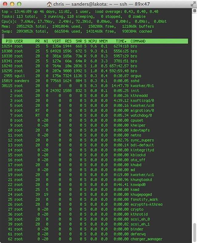
FIGURE 3.3 Monitoring Sensor CPU Usage with TOP

Memory

The amount of memory required for collection and detection is usually smaller than for analysis. This is because analysis often results in multiple analysts running several instances of the same tools successively. Generally, a sensor should have an abundance of memory, but this amount should increase drastically if a full cycle sensor is being deployed. Since memory can be difficult to plan for, it is often best to purchase hardware with additional memory slots to allow for future growth.

Just like was discussed earlier regarding CPU usage, tools like top or htop can be used to determine exactly how much memory certain applications utilize (Figure 3.4). Remember that it is critical that this assessment be done while the sensor is seeing traffic throughput similar to the load it will experience while in production.

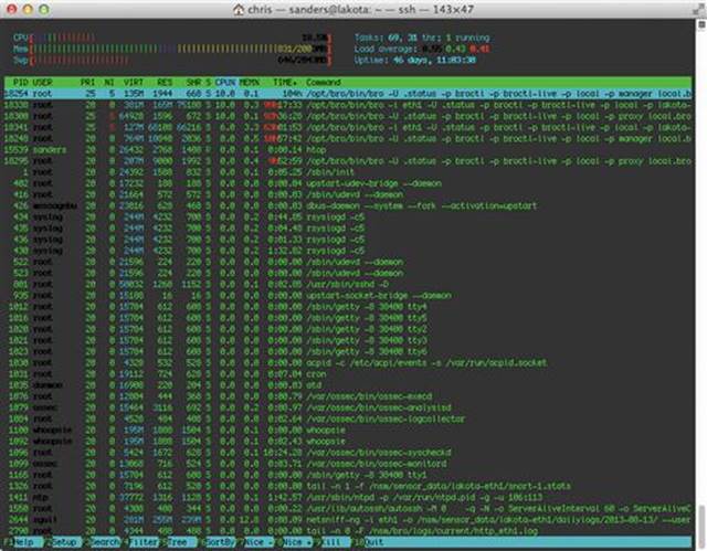
FIGURE 3.4 Monitoring Sensor Memory Utilization with HTOP

Practically speaking, memory is relatively inexpensive, and some of the latest network monitoring tools attempt to take advantage of that fact. Having a large amount of memory for your tools will help their performance under larger data loads.

Hard Disk Storage

One of the areas organizations have the most difficulty planning for is hard disk storage. This is primarily because there are so many factors to consider. Effectively planning for storage needs requires you to determine the placement of your sensor and the types of traffic you will be collecting and generating with the sensor. Once you’ve figured all of this out, you have to estimate future needs as the network grows in size. With all of that to consider, it’s not surprising that even after a sensor has been deployed, storage needs often have to be reevaluated.

The following series of steps can help you gauge the storage needs for a sensor. These steps should be performed for each sensor you are deploying.

Step One: Calculate the Traffic Collected

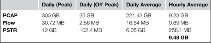
Utilizing a temporary sensor, you should begin by calculating data storage needs by determining the amount of NSM data collected over certain intervals. I like to attempt to collect at least 24 hours of data in multiple collection periods, with one collection period on a weekday and another on a weekend. This will give you an accurate depiction of data flow encompassing both peak and off-peak network times for weekdays and weekends. Once you’ve collected multiple data sets, you should then be able to average these numbers to come up with an average amount of data generated per hour.

In one example, a sensor might generate 300 GB of data PCAP in a 24-hour period during the week (peak), and 25 GB of data on the weekend (off peak). In order to calculate the daily average, we multiply the peak data total with the number of weekdays (300 GB x 5 Days = 1500 GB), and multiply the off peak data total with the number of weekend days (25 GB x 2 Days = 50 GB). Next, we add the two totals (1500 GB + 50 GB = 1550 GB), and find the average daily total by dividing that number by the total number of days in a week (1550 GB / 7 Days = 221.43 GB). This can then be divided by the number of hours in a day to determine the average amount of PCAP data generated per hour (221.43 GB / 24 Hours = 9.23 GB).

The result of these calculations for multiple data formats can be formatted in a table like the one shown in Table 3.2.

Table 3.2

Sensor Data Collection Numbers

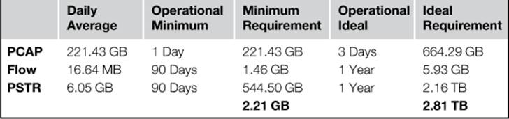
Step Two: Determine a Feasible Retention Period for Each Data Type

Every organization should define a set of operational minimum and ideal data retention periods for NSM data. The operational minimum is the minimal requirements for performing NSM services at an acceptable level. The operational ideal is set as a reasonable goal for performing NSM to the best extent possible. Determining these numbers depends on the sensitivity of your operations and the budget you have available for sensor hardware. When these numbers have been determined, you should be able to apply them to the amount of data collected to see how much space is required to meet the retention goals. We’ve taken the data from Table 3.2 and multiplied it with example minimum and ideal numbers. This data has been placed in Table 3.3.

Table 3.3

Required Space for Data Retention Goals

Step Three: Add Sensor Role Modifiers

In most production scenarios, the sensor operating system and tools will exist on one logical disk and the data that is collected and stored by the sensor will exist on another. However, in calculating total disk space required, you need to account for the operating system and the tools that will be installed. The storage numbers discussed up to this point assume a collection-only sensor. If you plan on deploying a half cycle sensor, then you should add an additional 10% to your storage requirements to accommodate for detection tools and the alert data generated from them. If you will be deploying a full cycle sensor, then you should add 25% for both detection and analysis tools and data. Once you’ve done this, you should add an additional 10-25% based upon the requirements for the operating system, as well as any anticipated future network growth. Keep in mind that these numbers are just general guidelines, and can vary wildly depending on the organization’s goals and the individual network. These modifiers have been applied to our sample data in Table 3.4.

Table 3.4

Completed Hard Disk Storage Assessment

Although I didn’t do this in Table 3.4, I always recommend rounding up when performing these calculations to give yourself plenty of breathing room. It is typically much easier to plan for additional storage before the deployment of a sensor rather than having to add more storage later.

While planning, it is important to keep in mind that there are numerous techniques for minimizing your storage requirements. The most common two techniques are varying your retention period for certain data types or simply excluding the collection of data associated with certain hosts or protocols. In the former, your organization might decide that since you are collecting three months of PSTR data, you only need twelve hours of FPC data. In the latter you may configure your full packet captures to ignore especially verbose traffic such as nightly backup routines or encrypted traffic such as SSL/TLS traffic. While both techniques have positives and negatives, they are the unfortunate outcome of making decisions in an imperfect world with limited resources. An initial tool you may use in the filtering of traffic to all of your sensor processes is the Berkeley Packet Filter (BPF). Techniques for using BPF’s to filter traffic will be discussed in Chapter 13.

Network Interfaces

The Network Interface Card (NIC) is potentially the most important hardware component in the sensor, because the NIC is responsible for collecting the data used for all three phases of the NSM Cycle.

A sensor should always have a minimum of two NICs. One NIC should be used for accessing the server, either for administration or analysis purposes. The other NIC should be dedicated to collection tasks. The NIC used for administration typically doesn’t need to be anything special, as it will not be utilized beyond that of a typical server NIC. The degree of specialization required for the collection NIC depends upon the amount of traffic being captured. With quality commodity NICs, such as the popular Intel or Broadcom units, and the correct configuration of a load balancing network socket buffer, such as PF_Ring, it is rather trivial to monitor up to 1 Gbps of traffic without packet loss.

The number of NICs used will depend on the amount of bandwidth sent over the link and the types of taps selected. It is important to remember that there are two channels on a modern Ethernet: a Transmit (TX) channel and a Receive (RX) channel. A standard 1 Gbps NIC is cable of transporting an aggregate 2 Gbps; 1 Gpbs in each direction, TX and RX. If a NIC sees less than 500 Mbps (in each direction), you should be relatively safe specifying a single 1 Gbps NIC for monitoring. We say “relatively” though, because a 1 Gbps NIC connected to a router with a 500 Mbps/500 Mbps uplink could buffer traffic for transmission, allowing peaks in excess of the uplink throughput to happen. Advanced network taps can assist in mitigating these types of performance mismatches. We will provide more guidance on network taps in the next section.

In order to gauge exactly what throughput you will need for your collection NIC, you should perform an assessment of the traffic you will be collecting. The easiest method to assess the amount of traffic on a given link will be to inspect, or to set up, some simple aggregate monitoring on your router or switch. The two most important aggregate numbers are:

• Peak to peak traffic (Measured in Mbps)

• Average bandwidth (throughput) per day (Measured in Mbps)

For example, you may have an interface that you plan to monitor that is a 1 Gbps interface, with an average throughput of 225 Mbps, an average transmit of 100 Mbps, an average receive of 350 Mbps, and with sustained bursts to 450 Mbps. Whatever NIC you plan to utilize should be able to handle the sustained burst total as well as the average throughput.

Caution

Traffic is bi-directional! A 1 Gbps connection has a maximum throughput of 2 Gbps - 1 Gbps TX and 1 Gbps RX.

An additional input into your sensor design will be the composite types of network protocol traffic you will be seeing across the specific link. This may vary depending on the time of day (e.g. backup routines at night), the time of year (e.g. students in session), and other variables. To do this, configure the SPAN port or network tap the sensor will be plugged into, and then plug a temporary sensor into it that has a high throughput NIC to determine the type of data traversing this link. Suggested methods of analysis include capturing and analyzing NetFlow data, or capturing PCAP data to replay through analysis tools offline.

These measurements should be taken over time in order to determine the peak traffic levels and types of traffic to expect. This should help you to determine whether you will need a 100 Mbps, 1 Gbps, 10 Gbps, or larger throughput NIC. Even at low throughput levels, it is important that you purchase enterprise-level hardware in order to prevent packet loss. The 1 Gbps NIC on the shelf at Wal-Mart might only be $30, but when you try to extract a malicious PDF from a stream of packets only to find that you are missing a few segments of data, you will wish you had spent the extra money on something built with quality.

To capture traffic beyond 1 Gbps, or to maximize the performance of your sensor hardware, there are a variety of advanced high performance network cards available. The three most common vendors ,from most to least expensive, are Napatech, Endace, and Myricom. Each of these cards families provides various combinations of a variety of high performance features such as on card buffers, hardware time stamping, advanced network socket drivers, GBIC interface options, and more. The enterprise NIC market is a very fast moving area. Currently, we recommend Myricom products, as they seem to be an incredible value and perform highly when paired with the propriety Myricom network socket buffer.

In cases where you find that your sensor is approaching the 10 Gbps throughput barrier, you will likely either have to reconsider the sensor placement, or look into some type of load-balancing solution. This amount of data being collected and written to disk could also cause some additional problems related to hard disk I/O.

Load Balancing: Socket Buffer Requirements

Once the traffic has made its way to the network card, special consideration must be paid to balancing the traffic within a sensor across the various processes or application threads. The traditional Linux network socket buffer is not suited to high performance traffic analysis; enter Luca Deri’s PF_Ring. The general goal of PF_Ring is to optimize the performance of network sockets through a variety of techniques such as a zero copy ring buffer where the NIC bypasses copying network traffic to kernel space by directly placing it in user space; thus saving the operating system an expensive context switch. This makes the data collection process faster and more efficient.

One way to conceptualize PF_Ring is to think of it taking your network traffic and fanning it out for delivery to a variety of tools. It can operate in two modes: either per packet round robin, or by ensuring an entire flow is delivered to a single process or thread within a sensor. In PF_Ring’s current implementation, you can generate a 5-tuple hash consisting of the source host, destination host, source port, destination port and protocol. This algorithm ensures that all of the packets for a single TCP flow and mock UDP/ICMP flows are handled by a specific process or thread.

While PF_Ring isn’t the only option for use with common detection tools like Bro, Snort, or Suricata, it is the most popular, and it is supported by all three of these.

For high performance sensor applications or designing sensors for operation in environments in excess of 1 Gbps, significant performance gains may be achieved through the use of aftermarket network sockets. With the sponsorship of Silicom, ntop.org now offers a high performance network socket designed for use with commodity Intel NICs called PF_Ring + DNA. Presently licensed per port, the PF_Ring + DNA performance tests are impressive and should be on your list of options to evaluate. Licensed per card, the Myricom after market driver for use with their own brand of card presently seems to be the best value.

SPAN Ports vs. Network Taps

Although they are not a part of the physical server that acts as a sensor, the device you utilize to get packets to the sensor is considered a part of the sensor’s architecture. Depending on where you place the sensor on your network, you will either choose to utilize a SPAN port or a Network Tap.

A SPAN port is the simplest way to get packets to your sensor because it utilizes preexisting hardware. A SPAN port is a function of an enterprise-level switch that allows you to mirror one or more physical switch ports to another port. In order to accomplish this, you must first identify the port(s) whose traffic is desirable to the sensor. This will most often be the port that connects an upstream router to the switch, but could also be several individual ports that important assets reside on. With this information in hand, you can configure the traffic inbound/outbound from this port to be mirrored to another port on the switch, either through a GUI or command line interface, depending on the switch manufacturer. When you connect your collection NIC on the sensor to this port, you will see the exact traffic from the source port you are mirroring from. This is depicted in Figure 3.5, where a sensor is configured to monitor all traffic from a group of network assets to a router by mirroring the port the router is attached to over to the sensor.

More Information

While port mirror is a common feature on enterprise-level switches, it is a bit harder to find on small office and home (SOHO) switches. Miarec maintains a great listing of SOHO switches with this functionality athttp://www.miarec.com/knowledge/switches-port-mirroring.

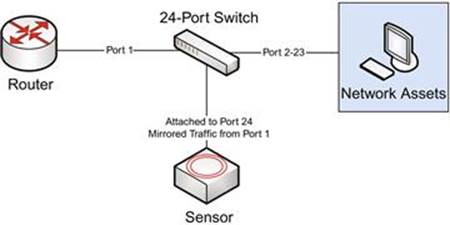
FIGURE 3.5 Using a SPAN Port to Capture Packets

Most switches allow a many-to-one configuration, allowing you to mirror multiple ports to a single port for monitoring purposes. When doing this, it’s important to consider the physical limits of the switch. For instance, if the ports on the switch are 100 Mbps, and you mirror 15 ports to one port for collection, then it is likely that the collection port will become overloaded with traffic, resulting in dropped packets. I’ve also seen some switches that, when sustaining a maximum load over a long time, will assume the port is caught in some type of denial of service or broadcast storm and will shut the port down. This is a worst-case scenario, as it means any collection processes attached to this port will stop receiving data.

Another method for getting packets to your sensor is the use of a network tap. A tap is a passive hardware device that is connected between two endpoints, and mirrors their traffic to another port designed for monitoring. As an example, consider a switch that is plugged into an upstream router. This connection utilizes a single cable with one end of the cable plugged into a port in the switch, and another cable plugged into a port on the router. Using a tap, there will be additional cabling involved. The end of one cable is plugged into a port on the switch, and the other end of that cable is plugged into a port on the tap. On the next cable, one end of the cable is plugged into a port on the tap, and the other end is plugged into a port on the router. This ensures that traffic is transmitted successfully between the router and the switch. This is shown in Figure 3.6.

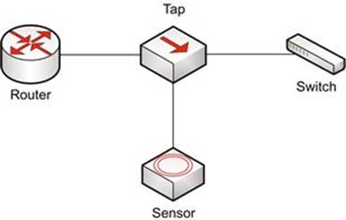
FIGURE 3.6 Using a Network Tap to Capture Packets

In order to monitor the traffic intercepted by the tap you must connect it to your sensor. The manner in which this happens depends on the type of tap being utilized. The most common type of tap is an aggregated tap. With an aggregated tap, a cable has one end plugged into a single monitor port on the tap, and the other end plugged into the collection NIC on the sensor. This will monitor bidirectional traffic between the router and switch. The other common variety of tap is the non-aggregated tap. This type will have two monitor ports on it, one for each direction of traffic flow. When using a non-aggregated tap, you must connect both monitor ports to individual NICs on the sensor. Both types of taps are shown in Figure 3.7.

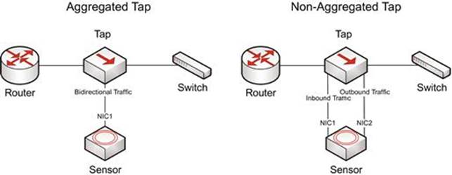
FIGURE 3.7 Aggregated and Non-Aggregated Taps

Taps are typically the preferred solution in high performance scenarios. They come in all shape and sizes and can scale up to high performance levels. You get what you pay for with taps, so you shouldn’t spare expense when selecting a tap to be used to monitor critical links.

While both taps and SPAN ports can get the job done, in most scenarios, taps are preferred to SPAN ports due to their high performance and reliability.

Bonding Interfaces

When using a non-aggregated tap, you will have at least two separate interfaces on your sensor. One interface monitors inbound traffic from the tap, and the other monitors outbound traffic. Although this gets the job done, having two separate data streams can make detection and analysis quite difficult. There are several different ways to combine these data streams using both hardware and software, but I prefer a technique called interface bonding. Interfacing bonding allows you to create a virtual network interface that combines the data streams of multiple interfaces into one. This can be done with software.

As an example, let’s bond two interfaces together in Security Onion. As you can see by the output shown in Figure 3.8, the installation of Security Onion I’m using has three network interfaces. Eth2 is the management interface, and eth0 and eth1 are the collection interfaces.

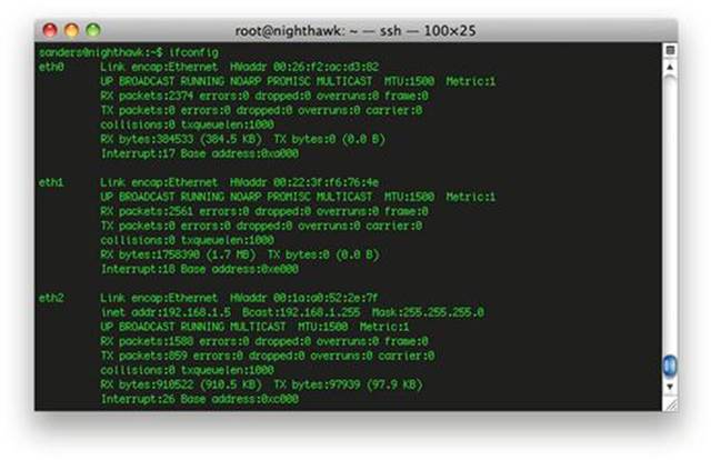
FIGURE 3.8 Network Interfaces on the System

For the purposes of this exercise, let’s assume that eth0 and eth1 are connected to a non-aggregated tap, and that they are both seeing unidirectional traffic. An example of the same traffic stream sniffed from both interfaces can be seen in Figure 3.9. In this figure, the results of an ICMP echo request and reply generated from the ping command are shown. In the top window, notice that only the traffic to 4.2.2.1 is seen, where as in the bottom window, only the traffic from 4.2.2.1 is seen.

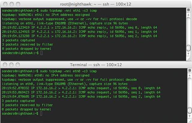
FIGURE 3.9 Unidirectional Traffic Seen on Each Interface

Our goal is to combine these interfaces into their own interface to make analysis easier. In Security Onion this can be done using bridge-utils, which is now included with it. You can set up a temporary bridge using the following commands:

sudo ip addr flush dev eth0

sudo ip addr flush dev eth1

sudo brctl addbr br0

sudo brctl addif br0 eth0 eth1

sudo ip link set dev br0 up

This will create an interface named br0. If you sniff the traffic of this interface, you will see that the data from eth0 and eth1 are now combined. The end result is a single virtual interface. As seen in Figure 3.10, while sniffing traffic on this interface we see both sides of the communication occurring:

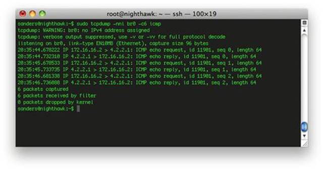
FIGURE 3.10 Bidirectonal Traffic from the Virtual Interface

If you wish to make this change persistent after rebooting the operating system, you will need to make a few changes to Security Onion, including disabling the graphical network manager and configuring bridge-utils on the /etc/network/interfaces file. You can read more about those changes here:

• http://code.google.com/p/security-onion/wiki/NetworkConfiguration

• https://help.ubuntu.com/community/NetworkConnectionBridge

Sensor Operating System

The most common sensor deployments are usually some flavor of Linux or BSD. Every flavor has its upsides and downsides, but it usually boils down to personal preference. Most people who have DoD backgrounds prefer something Red Hat based such as CentOS or Fedora, because the DoD mostly utilizes Red Hat Linux. A lot of the more “old school” NSM practitioners prefer FreeBSD or OpenBSD due to their minimalistic nature. While the particular flavor you choose may not matter, it is very important that you use something *nix based. There are a variety of reasons for this, but the most prevalent is that most of the tools designed for collection, detection, and analysis are built to work specifically on these platforms. In 2013, Linux seems to be the most popular overall choice, as hardware manufactures seem to universally provide up to date Linux drivers for their hardware.

Sensor Placement

Perhaps the most important decision that must be made when planning for NSM data collection is the physical placement of the sensor on the network. This placement determines what data you will be able to capture, what detection ability you will have in relation to that data, and the extent of your analysis. The goal of sensor placement is to ensure proper visibility into the data feeds that have been established as critical to the NSM process within the organization. If you are using the methods described in this book to make that determination, then you likely decided what data was the most important for collection by going through the applied collection framework discussed in chapter two.

There is no tried and true method for determining where to best place a sensor on the network, but there are several tips and best practices that can help you avoid common pitfalls.

Utilize the Proper Resources

Good security doesn’t occur in a vacuum within an organization, and sensor placement shouldn’t either. While the placement of a sensor is a goal of the security team, determining how to best integrate this device into the network is more within the realm of network engineering. With that in mind, the security team should make every effort to engage network engineering staff at an early stage of the placement process. Nobody knows the network better than the people who designed it and maintain it on a daily basis. They can help guide the process along by ensuring that the goals are realistic and achievable within the given network topology. Of course, in some cases the network engineering staff and the security team might consist of a solitary person, and that person might be you. In that case, it makes scheduling meetings a lot easier!

The document that is usually going to provide the most insight into the overall design of a network or individual network segment is the network diagram. These diagrams can vary wildly in detail and design, but they are critical to the process so that the network architecture can be visualized. If your organization doesn’t have network diagrams, then this would be a good time to to make that happen. Not only will this be crucial in determining visibility of the sensor, but it will also help in the creation of visibility diagrams for use by your analysts. We will talk about those diagrams later in this section.

Network Ingress/Egress Points

In the ideal case, and when the appropriate resources are available, a sensor should be placed at each distinct ingress/egress point into the network including Internet gateways, traditional VPNs, and partner links. In smaller networks, this may mean deploying a sensor at one border on the network edge. You will find that many large organizations have adopted a hub and spoke model where traffic from satellite offices are transported back to the main office via VPN, MPLS, or other point-to-point technology to centrally enforce network monitoring policies. This setup will require a wider dispersion of sensors for each of these ingress/egress points.

The diagram shown in Figure 3.11 represents a network architecture that might be found in a larger organization with many ingress/egress points. Note that all of the routers shown in this diagram are performing Network Address Translation (NAT) functions.

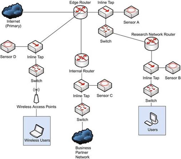
FIGURE 3.11 Placing Sensors at Network Ingress/Egress Points

In this case, notice that there are four separate sensors deployed:

A. At the corporate network edge

B. At the research network edge

C. At the ingress point from a business partner network

D. At the edge of the wireless network

Ultimately, any truly negative activity occurring on your network (except for physical theft of data) will involve data being communicated into or out of the network. With this in mind, sensors placed at these ingress/egress points will be positioned to capture this data.

Visibility of Internal IP Addresses

When performing detection and analysis, it is critical to be able to determine which internal device is the subject of an alert. If your sensor is placed on the wrong side of a NAT device such as a router, you could be shielded from this information.

The diagram shown in Figure 3.12 shows two different scenarios for a single network. The network itself is relatively simple, in which the corporate network exists behind an internal router that forms a DMZ between itself and the edge router, which connects to the Internet.

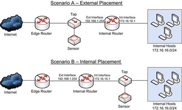
FIGURE 3.12 A Simple Network with Two Sensor Placement Examples

The devices downstream from the internal router have IP addresses in the 172.16.16.0/24 range. The router has an internal LAN IP address of 172.16.16.1, and an external WAN interface of 192.168.1.254. This forms a DMZ between the internal router and the edge router.

There are two scenarios shown here. In scenario A, the sensor is placed upstream from the internal router, in the DMZ. The alert shown in Figure 3.13 represents what happens when a user in the group of internal hosts falls victim to a drive-by download attack that causes them to download a malicious PDF file associated with the Phoenix exploit kit.

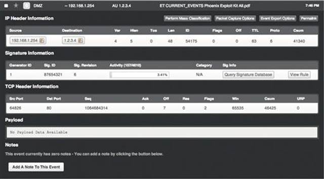
FIGURE 3.13 A User in Scenario A Generating an Alert

This alert indicates that the device at 192.168.1.254 attempted to download a PDF from the host at 1.2.3.4, and that this PDF is linked to the Phoenix exploit kit. The problem with this is that 192.168.1.254 is the external IP address of the internal router, and this doesn’t give us any indication of which internal host actually initiated this communication. Pulling NetFlow data yields the results shown in in Figure 3.14.

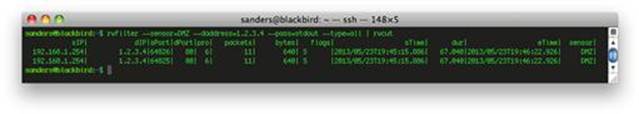
FIGURE 3.14 NetFlow Data from Scenario A

With this sensor placement, you will not see any internal IP addresses in the 172.16.16.0/24 range. This is because the internal router is utilizing NAT to mask the IP addresses of the hosts inside that network. The data collected by this sensor gives us absolutely no ability to adequately investigate the alert further. Even if you had other data sources available such as antivirus or HIDS logs, you wouldn’t know where to begin looking. This becomes especially complex on a network with hundreds or thousands of hosts on a single network segment.

In scenario B, the sensor is placed downstream from the router. Figure 3.15 shows that the same malicious activity generates the same alert, but provides different information.

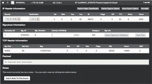
FIGURE 3.15 A User in Scenario B Generating an Alert

Here we can see the same external address of the site hosting the malicious file (1.2.3.4), but instead of the external IP of the internal router, we actually see the proper internal IP of the host that needs to be examined for further signs of infection. NetFlow data shows this as well in Figure 3.16.

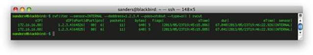
FIGURE 3.16 NetFlow Data from Scenario B

It is critical that your collected data serves an analytic purpose. This example applies just as much to sensors placed within internal network segments as it does to network segments that are only one hop away from the Internet. You should always ensure that you are on the right side of routing devices.

Proximity to Critical Assets

In the introductory material of this book, we discussed how casting a wide net and attempting to collect as much data as possible can be problematic. This should be taken into account when you place your sensors. If you’ve taken the time to properly determine which data feeds are mission critical in light of the threats your organization faces, you should have defined which assets are the most important to protect. With this in mind, if you have limited resources and can’t afford to perform collection and detection at all of your network’s ingress/egress points, you can logically place your sensors as close as possible to these critical assets.

Figure 3.17 shows an example of a mid-sized network belonging to a biomedical research firm. In planning for collection, this firm decided that the devices they are most concerned with protecting are those within the research network, as they contain the organization’s intellectual property. This image shows three possible sensor placements.

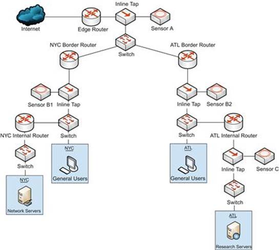
FIGURE 3.17 A Mid-Sized Network with Three Sensor Placement Examples

In an ideal world with unlimited money, time, and resources we might want to deploy all of these sensors in order gain the best visibility of the network. However, that just isn’t always realistic.

Our first thought might be to place a sensor on the network edge, which is what is depicted with sensor A. If this is the only sensor placed on this network, it becomes responsible for collection and detection for the entire enterprise. As we’ve already discussed, this model doesn’t always scale well and ultimately results in incredibly expensive hardware and an inability to perform thorough collection, detection, and analysis.

Next, we might consider placing the sensors at the border of each physical site, as shown with sensors B1 and B2. This essentially splits the workload of sensor A in half, with a sensor for both the NYC and ATL locations. While this does have some performance benefits, we still have two sensors that are responsible for processing a wide variety of data. The sensor at the NYC site alone must have detection signatures that will encompass possible threats related to different servers on the network servers segment, as well as users. This still isn’t focusing on the biggest perceived threat to the organization.

Finally, we come to sensor C, which is placed so that it has visibility into the research network at the ATL location. This segment contains users who are actively involved in research, and the servers where their data is stored. Based upon the risk analysis that was completed for this network, the biggest threat to the organization would be a compromise on this network segment. Therefore, this is where I would place my first sensor. Because this network is smaller in size, less powerful hardware can be used. Additionally, detection mechanisms can be deployed so that a trimmed down set of signatures that only encompass the technologies on this part of the network can be used.

In a scenario like this one, it would be ideal if the resources were available to place more than one sensor. Perhaps a combination of sensor A and C might be the best ‘bang for your buck.’ However, if the assets that represent the highest level of risk in the company are those in research server segment, then that is a great place to start.

Creating Sensor Visibility Diagrams

When a sensor has been placed on the network, it is critical that analysts know where that sensor exists in relation to the assets it is responsible for protecting, as well as other trusted and untrusted assets. This is where network diagrams become incredibly useful for reference during an investigation.

Most organizations would be content to take a network diagram that was created by the systems administration or network engineering staff and point to where the sensor is physically or logically placed. While this can be useful, it isn’t really the most efficient way to present this information to an NSM analyst. These diagrams aren’t usually made for the NSM analyst, and can often induce a state of information overload where non-relevant information prevents the analyst from fully understanding the exact architecture as it relates to protected and trusted/untrusted assets. In other terms, I would consider giving an NSM analyst a network engineering diagram equivalent to providing a cook with the DNA sequence of a tomato. If the cook wants to know about the particulars of what comprises a tomato’s flavor then he can reference that information, but in most cases, he just needs the recipe that tells him how to cook that tomato. With NSM analysis, it is always beneficial if detailed network diagrams are available to analysts, but in most cases a simplified diagram is better suited to their needs. The ultimate goal of the sensor visibility diagram is for an analyst to be able to quickly assess what assets a particular sensor protects, and what assets fall out of that scope.

A basic sensor visibility diagram should contain AT LEAST the following components:

• The high-level logical overview of the network

• All routing devices, proxies, or gateways that affect the flow of traffic

• External/Internal IP addresses of routing devices, proxies, and gateways

• Workstations, servers or other devices -- these should be displayed in groupings and not individually, unless they are particularly critical devices

• IP address ranges for workstation, server, and device groupings

• All NSM sensors, and appropriately placed boxes/areas that define the hosts the sensor is responsible for protecting. These boxes will usually be placed to define what hosts the sensor will actually collect traffic from. While the traffic from a nested subnet might only show the IP address of that subnet’s router’s external interface, the traffic will still be captured by the sensor unless otherwise excluded.

As an example, let’s consider the network that was described in Figure 3.17 earlier. I’ve redrawn this image in Figure 3.18 to represent the visibility of each sensor, incorporating the items listed above. The differing zones can typically be most effectively defined by colored or shaded boxes, but since this book is printed in black and white, I’ve used boxes with different types of line dashes to represent each monitored zone. In this case, each sensor is monitoring all of the traffic in the subnets nested below its subnet, so each zone is overlapping the zone for the upstream network.

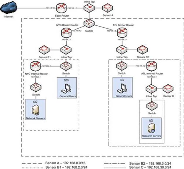
FIGURE 3.18 A Sensor Visibility Diagram

I would often have these diagrams laminated and placed at an analyst’s desk for quick reference during an investigation. They work great for a quick reference document, and can be a launching point for an analyst to find or request additional documentation relevant to the investigation, such as a more detailed diagram of a specific network segment or information associated with a particular trusted host.

Securing the Sensor

In the realm of sensitive network devices, the security of the sensor should be considered paramount. If your sensor is storing full packet capture data, or even just PSTR data, it is very likely that these files will contain incredibly sensitive network information. Even an unskilled attacker could use these files to extract entire files, passwords, or other critical data. An attacker could even use a sensor that is only storing session data to help them garner information about the network that might allow them to expand their foothold within the network. Several steps that can be taken to ensure the sanctity of your sensors.

Operating System and Software Updates

The single most important thing you can do to aid in the security of any system is to ensure that the software running on it and the underlying operating system are both up to date with the latest security patches. Even though your sensors shouldn’t be visible from the Internet, if your network gets compromised through some other means and an attacker can move laterally to a sensor via a months-old remote code execution vulnerability in your operating system, it’s game over.

I’ve seen many instances where people neglect patching sensor software and operating systems because the sensor doesn’t have Internet access. As a result, it becomes too much of a hassle to perform updates on a regular basis. In such instances, one solution is to set up some type of satellite update server within your network to ensure these updates are occurring in a timely manner. While this is extra management overhead, it does reduce a significant amount of risk to your sensors if they are not being updated frequently enough. One other solution would be to limit access to those domains required for software and system updates with the use of an internal web proxy, but this may prove challenging based on the placement of your sensor in the network.

Operating System Hardening

In addition to ensuring that the operating system of your sensor is up to date, it is critical that it is based upon secure configuration best practices before sensor software is even installed. There are several approaches to operating system security best practices. If your organization falls under any type of formal compliance standard such as HIPAA, NERC CIP, or PCI, then it is likely that you already employ some type of secure OS configuration standards. Federal and Defense sector agencies are also no stranger to these, as operating system security is enforced via any number of certification and accreditation processes, such as DIACAP or DITSCAP.

If you aren’t guided by any formal compliance standard, there are several publicly available resources that can serve as a good starting point. Two of these that I really like are the Center for Internet Security (CIS) benchmarks (http://benchmarks.cisecurity.org/) and the NSA Security Guides for Operating Systems (http://www.nsa.gov/ia/mitigation_guidance/security_configuration_guides/operating_systems.shtml).

Limit Internet Access

In most instances, your sensor should not have unfettered Interner access. If the sensor were to become compromised, this would make it trivially easy for an attacker to exfiltrate sensitive data from the sensor. I typically do not provide Internet access to sensors at all, although in some cases Internet access can be limited to only critically important domains (such as those required for software and system updates) with the use of an internal web proxy.

Importantly, your sensor processes will most likely be configured to download IDS signatures or reputation-based intelligence from the Internet at periodic intervals. Additionally, accessing data sources for intelligence services, such as Bro’s real-time usage of the Team Cymru Malware Hash Registry and the International Computer Science Institutes SSL Observatory, is a growing trend. You should ensure that your sensor can receive this data, but it might be preferable to have a single system configured to download these updates, and have sensors pointed to that internal device for updates.

Minimal Software Installation

A sensor is a specialized piece of hardware designed for a specific purpose. This specialization warrants that only necessary software be installed on the sensor. We recommend using a minimal operating system installation and only installing what software is needed to perform the required collection, detection, and analysis tasks for your type of sensor deployment. Furthermore, any unneeded services should be disabled and additional unused packages installed with the operating system should be removed. This ultimately increases sensor performance, and minimizes the potential attack surface.

The most common mistake I see in slimming down a server installation is when a sensor administrator forgets to remove compilers from a sensor. It is often the case that a compiler will be required to install NSM tools, but under no circumstances should the compiler be left on this system, as it provides an additional tool for an attacker to use against your network should the sensor be compromised. In a best case scenario, sensor tools are actually compiled on another system and pushed out to the sensor rather than being compiled on the sensor itself.

VLAN Segmentation

Most sensors should have at least two network connections. The first interface is used for the collection of network data, while the second will be used for the administration of the sensor, typically via SSH. While the collection interface shouldn’t be assigned an IP address or be allowed to talk on the network at all, the administration interface will be required to exist logically on the network at some location. If the network environment supports the segmentation of traffic with Virtual Local Area Networks (VLANs), then this should be taken advantage of, and the sensor management interface placed into a secure VLAN that is only accessible by the sensor administrator.

Host-Based IDS

The installation of some form of host-based intrusion detection (HIDS) on the sensor is critical. These systems provide detection of modifications to the host through a variety of means, including the monitoring of system logs and system file modification detection. Several commercial varieties of HIDS exist, but there are also free pieces of software available, such as OSSEC or the Advanced Intrusion Detection Environment (AIDE). Keep in mind that the HIDS software is used to detect a potential intrusion on the system it resides on, so the logs it generates should be sent to another server on the network. If they are stored locally and only periodically examined, this presents an opportunity for an attacker to modify or delete these logs before they can be examined.

Two-Factor Authentication

As an attacker, an NSM sensor is a target of great value. The raw and processed network data found on a sensor can be used to orchestrate or further a variety of attacks. Therefore, it is important to protect the authentication process used to access the sensor. Using a password-only authentication presents a scenario in which an attacker could harvest that password from another source and then access the sensor. Because of this, having two forms of authentication for sensors is recommended.

Network-Based IDS

It is crucial that the administration interface of the sensor be monitored as a high value network asset. It should come as no surprise that one of the best ways to do this is to subject this interface to the same NIDS detection used for the rest of the network. Of course, this software is probably running on the sensor itself. The easy solution is to mirror the administration interface’s network traffic to the monitoring interface. This is an easy step to take, but one that is often overlooked.

One of the best things you can do to ensure that your sensor isn’t communicating with any unauthorized hosts is to identify which hosts are permitted to talk to the sensor and create a Snort rule that will detect communication with any other device. For example, assuming that a sensor at 192.168.1.5 is only allowed to talk to the administrator’s workstation at 192.168.1.50 and the local satellite update server at 192.168.1.150, the following rule would detect communication with any other host:

alert ip ![192.168.1.50,192.168.1.150] any <> 192.168.1.50 any (msg:”Unauthorized Sensor Communication”; sid:5000000; rev:1;)

Conclusion

There is a lot of planning and engineering that goes into proper sensor creation, placement, and capacity planning. Like many topics, this is something that could nearly be its own separate book. This chapter was intended to provide an overview of the main concepts that should be considered when performing those actions. In addition to the concepts introduced here, it is a good practice to speak with colleagues and other organizations to see how they’ve deployed their sensors in light of their organizational goals and network architecture. This will provide a good baseline knowledge for determining the who, what, when, where, and why of NSM sensors.