Applied Network Security Monitoring: Collection, Detection, and Analysis (2014)
SECTION 1. Collection
CHAPTER 5. Full Packet Capture Data
Abstract
The type of NSM data with the most intrinsic value to the analyst is Full Packet Capture (FPC) data. FPC data provides a full accounting for every data packet transmitted between two endpoints. This chapter begins with an overview of the importance of full packet capture data. We will examine several tools that allow for full packet capture of PCAP data, including Netsniff-NG, Daemonlogger, and Dumpcap. This will lead to a discussion of discuss different considerations for the planning of FPC data storage and maintenance of that data, including considerations for trimming down the amount of FPC data stored.
Keywords
Network Security Monitoring; Collection; Packets; FPC; Full Packet Capture; Data; Dumpcap; Netsniff-NG; Daemonlogger; Throughput; Rwfilter; Rwcount; Rwstats
The type of NSM data with the most intrinsic value to the analyst is Full Packet Capture (FPC) data. FPC data provides a full accounting for every data packet transmitted between two endpoints. If we compare the investigation of computer-related crime to human-focused crime, having FPC data from a device under investigation would be equivalent to having a surveillance-video recording of a human suspect under investigation. Ultimately, if an attacker accesses a system from the network, there will be evidence of it within FPC data.
FPC data can be quite overwhelming due to its completeness, but it is this high degree of granularity that is valuable when it comes to providing analytic context. It does come with a price, however, as it can be quite storage intensive to capture and store FPC data for an extended period of time. Some organizations find that they simply don’t have the resources to effectively incorporate FPC data into their NSM infrastructure.
The most common form of FPC data is the PCAP data format (Figure 5.1). The PCAP format is supported by most open source collection, detection, and analysis tools and has been the gold standard for FPC data for quite a while. Several libraries exist for creating software that can generate and interact with PCAP files, but the most popular is Libpcap, which is an open source packet capture library that allows applications to interact with network interface cards to capture packets. Originally created in 1994, its main objective was to provide a platform-independent API that could be used to capture packets without the need for operating system specific modules. A large number of applications used in packet collection and analysis utilize Libpcap, including several of the tools discussed in this book, like Dumpcap, Tcpdump, Wireshark, and more. Since libraries like Libpcap make the manipulation of PCAP data so easy, often other NSM data types, such as statistical data or packet string data are generated from PCAP data.
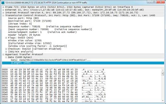
FIGURE 5.1 Sample PCAP Data as seen in Wireshark
Recently, the PCAP-NG format has evolved as the next version of the PCAP file format. PCAP-NG provides added flexibility to PCAP files, including allowing for comments to be inserted into packet captures (Figure 5.2). This feature is incredibly helpful to analysts when storing examined files for later analysis by themselves or other analysts. Most of the tools mentioned in this book support PCAP-NG.
From the Trenches
You can determine the format of a packet capture file by using the capinfos tool that is provided with Wireshark (which we will talk about more in Chapter 13). To do this, execute the command capinfos –t < file >. If the file is just a PCAP file, capinfos will tell you that it is a “libpcap” file. If it is a PCAP-NG file, it will refer to it as “pcapng.”
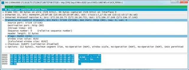
FIGURE 5.2 A Commented Packet Leveraging PCAP-NG
In this chapter we will explore several popular FPC collection solutions and highlight some of the benefits of each one. In addition to this, we will examine some strategies for implementing FPC solutions into your network in the most economical manner possible.
Dumpcap
One of the easiest ways to get up and running with full packet capture is by utilizing Dumpcap. The Dumpcap tool is included with Wireshark, which means that most analysts already have it on their system whether they know it or not. Dumpcap is a simple tool designed solely for the purpose of capturing packets from an interface and writing them to disk. Dumpcap utilizes the Libpcap packet capture library to capture packets and write them in PCAP-NG format.
If you are using Security Onion then Wireshark is already installed, which means that you already have Dumpcap. If not, then you can download the Wireshark suite from http://www.wireshark.org. Once you’ve downloaded and installed Wireshark (along with the bundled Libpcap driver, required for packet capture), you can begin logging packets by invoking the Dumpcap tool and specifying a capture interface, like this:
dumpcap –i eth1
This command will begin capturing packets and writing them to a randomly named file in the current working directory, and will continue to do so until stopped. Dumpcap provides some other useful options for crafting how packet data is stored and captured:
• -a < value >: Specifies when to stop writing to a capture file. This can be time duration, a file size, or a number of written files. Multiple conditions can be used together.
• -b < options >: Causes Dumpcap to write to multiple files based upon when certain criteria are met. This can be time duration, a file size, or a number of written files. Multiple conditions can be used together.
• -B < value >: Specifies the buffer size, which is the amount of data stored before writing to disk. It is useful to attempt to increase this if you are experiencing packet loss.
• -f < filter >: Berkeley Packet Filter (BPF) command(s) for filtering the capture file.
• -i < interface >: Capture packets from the specified interface
• -P: Save files as PCAP instead of PCAP-NG. Useful when you require backwards compatibility with tools that don’t support PCAP-NG yet.
• -w < filename >: Used to specify the output file name.
In order to get this command more “production ready”, we might invoke the command like this:
dumpcap –i eth1 –b duration:60 –b files:60 –w NYC01
This command will capture packets from the eth1 interface (-i eth1), and store them in 60 files (-b files:60), each containing 60 seconds worth of captured traffic (-b duration:60). When the 60th file has been written, the first file starts being overwritten. These files will be numbered using the string we specified and adding the number of the file, and a date time stamp (-w NYC01).
While Dumpcap is simple to get up and running, it does have its limitations. First of all, it doesn’t always stand up well in high performance scenarios when reaching higher throughput levels, which may result in dropped packets. In addition, the simplicity of the tool limits its flexibility. This is evident in the limited number of configuration options in the tool. One example of this can be found in how Dumpcap outputs captured data. While it will allow you to specify text to prepend to packet capture filenames, it does not provide any additional flexibility in controlling the naming of these files. This could prove to be problematic if you require a specific naming convention for use with a custom parsing script or a third party or commercial detection or analysis tool that can read PCAP data.
Dumpcap is a decent FPC solution if you are looking to get up and running quickly with a minimal amount of effort. However, if you require a great degree of flexibility or are going to be capturing packets on a high throughput link, you will probably want to look elsewhere.
Daemonlogger
Designed by Marty Roesch, the original developer of the Snort IDS, Daemonlogger is a packet logging application designed specifically for use in NSM environments. It utilizes the Libpcap packet capture library to capture packets from the wire, and has two operating modes. Its primary operating mode is to capture packets from the wire and write them directly to disk. Its other mode of operation allows it to capture packets from the wire and rewrite them to a second interface, effectively acting as a soft tap.
The biggest benefit Daemonlogger provides is that, like Dumpcap, it is simple to use for capturing packets. In order to begin capturing, you need only to invoke the command and specify an interface.
daemonlogger –i eth1
This option, by default, will begin capturing packets and logging them to the current working directory. Packets will be collected until the capture file size reaches 2 GB, and then a new file will be created. This will continue indefinitely until the process is halted.
Daemonlogger provides a few useful options for customizing how packets are stored. Some of the more useful options include:
• -d: Run as a daemon
• -f < filename >: Load Berkeley Packet Filters (BPF’s) from the specified file
• -g < group >: Run as the specified group
• -i < interface >: Capture packets from the specified interface
• -l < directory >: Log data to a specified directory
• -M < pct >: In ring buffer mode, log packet data to a specified percentage of volume capacity. To activate ring buffer mode, you’ll also need to specify the -r option.
• -n < prefix >: Set a naming prefix for the output files (Useful for defining sensor name)
• -r: Activates ring buffer mode
• -t < value >: Roll over the log file on the specified time interval
• -u < user >: Run as the specified user
With these options available, a common production implementation might look like this:
daemonlogger –i eth1 –d –f filter.bpf –l /data/pcap/ -n NYC01
When this command is invoked, Daemonlogger will be executed as a daemon (-d) that logs packets captured from interface eth1 (-i eth1) to files in the directory /data/pcap (-l /data/pcap). These files will be prepended with the string NYC01 to indicate the sensor they were collected from (-n NYC01). The data that is collected will be filtered based upon the BPF statements contained in the file filter.bpf (-f filter.bpf).
Daemonlogger suffers from some of the same deficiencies as Dumpcap when it comes to performance. While Daemonlogger does perform better than Dumpcap at higher throughput levels, it can still suffer as throughput levels increase to those seen in some larger enterprise environments.
Daemonlogger also provides limited ability to control output file names. It will allow you to specify text to prepend to packet capture files, but it follows that text with the time the capture was created in epoch time format. There is no way to specify the date/time format that is included in the file name. Additional scripting can be done to rename these files after they’ve been created, but this is another process that will have to be managed.
Daemonlogger currently sets itself apart from the crowd by offering a ring buffer mode to eliminate the need for manual PCAP storage maintenance. By specifying the –r –M < pct > option in Daemonlogger, you can tell it to automatically remove older data when PCAP storage exceeds the specified percentage. In certain cases this might be essential, however if you’re already gathering other types of data, this storage maintenance is probably already being taken care of by other custom processes, like the ones we will talk about later in this chapter.
Once again, Daemonlogger is a great FPC solution if you are looking to get up and running quickly with a minimal amount of effort. It is incredibly stable, and I’ve seen it used successfully in a variety of enterprise environments. The best way to determine if Daemonlogger is right for you is to give it a try on a network interface that you want to monitor and see if you experience any packet loss.
Netsniff-NG
Netsniff-NG is a high-performance packet capture utility designed by Daniel Borkmann. While the utilities we’ve discussed to this point rely on Libpcap for capture, Netsniff-NG utilizes zero-copy mechanisms to capture packets. This is done with the intent to support full packet capture over high throughput links.
One of the neat features of Netsniff-NG is that it not only allows for packet capture with the RX_RING zero-copy mechanism, but also for packet transmission with TX_RING. This means that it provides the ability to read packets from one interface and redirect them to another interface. This feature is made more powerful with the ability to filter captured packets between the interfaces.
In order to begin capturing packets with Netsniff-NG, we have to specify an input and output. In most cases, the input will be a network interface, and the output will be a file or folder on disk.
netsniff-ng –i eth1 –o data.pcap
This command will capture packets from the eth0 interface (-i eth1) and write them to a file called data.pcap in the currently directory (-o data.pcap) until the application is stopped. If you execute this command, you’ll also notice that your screen fills with the contents of the packets you are capturing. In order to prevent this behavior, you’ll need to force Netsniff-NG into silent mode with the -s flag.
When you terminate the process (which can be done by pressing Ctrl + C), Netsniff-NG will generate some basic statistics related to the data it’s captured. We see these statistics in Figure 5.3.
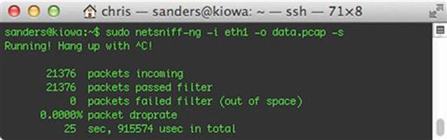
FIGURE 5.3 Netsniff-NG Process Output
Netsniff-NG provides a lot of the features found in the other FPC applications we’ve discussed. Some of these options include:
• -g < group >: Run as the specified group
• -f < file name >: Load Berkeley Packet Filters (BPF’s) from a specified file
• -F < value >: A size or time interval used to determine when to end capture in single-file mode, or roll over to the next file in ring buffer mode.
• -H: Sets the process priority to high
• -i < interface >: Capture packets from the specified interface
• -o < file >: Output data to the specified file
• -t < type >: Only handle packets of defined types (host, broadcast, multicast, outgoing)
• -P < prefix >: Set a naming prefix for the output files (Useful for defining sensor name)
• -s: Run silently. Don’t print capture packets to screen
• -u < user >: Run as the specified user
With these options available, a common production implementation might look like this:
netsniff-ng -i eth1 –o /data/ -F 60 -P “NYC01”
This command will run Netsniff-NG in ring buffer mode, which is noted by the usage of an output directory instead of a file name in the –o parameter (-o /data/). This will generate a new PCAP file every 60 seconds (–F 60), and every file will be prefixed with the sensor name NYC01 (-P “NYC01”).
In our testing, Netsniff-NG is the best performing FPC utilities in this book when it comes to very high throughput links. It performs so well, that it is included with Security Onion as the de facto FPC utility.
Choosing the Right FPC Collection Tool
We have discussed three unique FPC solutions, and in each description mentioned the overall performance of each tool. While Dumpcap and Daemonlogger will generally work fine in most situations with little to no packet loss, you will need a tool like Netsniff-NG to operate in environments with extremely high sustained traffic rates. Without scaling up your collection tools to meet your throughput requirements, you will be wasting CPU cycles and gathering incomplete data. There is nothing more frustrating for an analyst than trying to reassemble a data stream only to find that a packet is missing and your efforts are all for naught.
The history of FPC collection tools mostly revolves around which can generate data “the best”. While sometimes “best” is a reference to being feature rich, it has classically been that new FPC solutions are created to meet the requirements of newer, faster networks. This is not to say that the best FPC collection tool is the one that can ingest data the fastest, but instead the one that drops the least amount of packets on your sensor and that also contains enough features to ensure that data is stored in a format accessible by your detection and analysis tools.
The three tools mentioned earlier are included in this book because they are all proven to get the job done in various network environments, and are a few of the most well-known and widely deployed free solutions. With that in mind, you must choose the best fit for your organization based upon the criteria that are the most important to you.
Planning for FPC Collection
Collection of FPC data should take high priority when architecting your sensor for a multitude of reasons. One reason for this is that you can generate almost all other major data types from previously collected FPC data. With that said, FPC data is a “primary” data type that is always collected directly off the wire. FPC data will always be the largest of any data type per time quanta. This means that for any given amount of time, the amount of hard disk space that is consumed by FPC data will surpass that of any other data type. This is not to say that FPC data will always take up the vast percentage of your disk. Many organizations place an extraordinary amount of value in retrospective log analysis and correlation, and as such, can often devote an equal or larger amount of disk space to other types of logs, like Bro logs. Of course, the result might be that you can only store 24 hours of PCAP data compared to the 1 year of Bro logs. The takeaway here is that a lot of the data you collect will either be derived from PCAP data or will be affected by its expansive storage requirements.
The key consideration you must keep in mind when deploying an FPC solution is throughput, or the average rate of network traffic over the interface(s) that you’re monitoring. Determining the throughput over a particular monitor port should be done before the first purchase of a sensor is made to ensure that the sensor will have the resources necessary to support collection and detection at the scale necessary. Attempting to engineer these requirements for a sensor after you’ve bought hardware is usually a recipe for disaster.
Storage Considerations
The first and most obvious consideration when generating FPC data is storage. PCAP takes up a lot of space relative to all other data types; so determining the amount of FPC data you want to store is critical. This decision begins by choosing a retention strategy that is either time-based or size-based.
A time-based strategy says that you will retain PCAP data for at LEAST a specific time interval, for example, 24 hours. A size-based strategy says that you will retain a minimum amount of PCAP data, usually allocated by a specific hard drive volume, for example, 10 TB of PCAP data (limited by a 10 TB RAID array). With both of these strategies, your organization should attempt to define operational minimums and operational ideals. The operational minimum is the minimal requirement for performing NSM services at an acceptable level and defines the time or size unit representing the least amount of data you can store. The operational ideal is set as a reasonable goal for performing NSM to the best extent possible and defines the time or size unit representing the amount of data you would like to store in an ideal situation. In doing this, you should always have the minimum amount, but strive for the ideal amount.
Deciding between a time- or size-based FPC data collection can depend on a variety of factors. In some regulated industries where specific compliance standards must be met, an organization may choose to use time-based FPC collection to align with those regulations, or simply because their organization is more attuned to store data based upon time intervals. In organizations where budgets are tighter and hardware is limited, NSM staff may choose to use a size-based strategy due to hard limits on available space. It is also common to see organizations use a size-based strategy on networks that are very diverse or rapidly growing, due to an inability to accurately gauge the amount of storage required for time-focused collection.
When planning for time-based retention, in theory, gauging the average throughput across an interface can allow you to determine how much data, per time interval, that you can store given a fixed amount of drive space. For example, if you determine that your interface sees 100 MB/s throughput on average and you have 1 TB of hard drive space reserved, you can theoretically store over 24 days of FPC data. However, it is a common pitfall to rely solely on the average throughput measurement. This is because this measurement doesn’t account for throughput spikes, which are short periods of time where throughput might dramatically increase. These spikes may occur for a number of reasons, and might be a result of regularly scheduled events like off site backups or application updates, or random events such as higher than average web browsing activity. Since FPC is a primary data type, these spikes can also result in an increase of other data that is derived from it. This compounds the effect of data spikes.
Due to the nature of network traffic, it is difficult to predict peak throughput levels. Because of this, organizations that choose a time-based retention plan are forced to choose a time interval that is considerably shorter than their hardware can handle in order to provide an overflow space. Without that overflow, you risk losing data or temporarily toppling your sensor.
Managing FPC data based on the total amount of stored data is a bit more straight forward and carries with it inherent safety features. With this method, you define the maximum amount of disk space that FPC data can occupy. Once the stored data reaches this limit, the oldest FPC data is removed to make room for newly collected data. As we saw before, Daemonlogger is an FPC solution that has this feature built in.
Calculating Sensor Interface Throughput with Netsniff-NG and IFPPS
We’ve talked a lot about how the collection and storage of FPC data depends on being able to reliably determine the total throughput of a sensor’s monitoring interface. Now, we will look at methods for calculating throughput statistics. The first method involves using a tool called ifpps, which is a part of the Netsniff-NG suite of tools. In Security Onion, Netsniff-NG is installed without ifpps, so if you want to follow along you will need to install it manually by following these steps:
1. Install the libncurses-dev prerequisite with APT
sudo apt-get install libncurses-dev
2. Download Netsniff-NG with GIT
git clone https://github.com/borkmann/netsniff-ng.git
3. Configure, Make, and Install only ifpps
./configure
make && sudo make install ifpps_install
After installing ifpps, you can make sure it installed correctly by running it with the –h argument to see its possible arguments, or just cut to the chase and run this command, which will generate a list of continuously updating network statistics;
ifpps -d < INTERFACE >
Ifpps will generate statistics detailing the current throughput of the selected interface, as well as other data related to CPU, disk I/O and other system statistics. A sample of this output is shown in Figure 5.4.
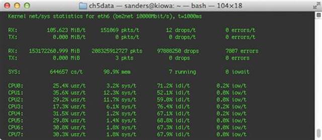
FIGURE 5.4 Generating Network Statistics with ifpps
The “/t” seen beside each statistic represents the time interval at the top right of the output and can be changed prior to execution using the -t option. The default time value is 1000ms.
Ifpps will give you a live snapshot of an interface’s throughput at any given point in time, which can be a useful statistic when combined with a large sample size. Using this method, you want to ensure that you collect multiple peak and off-peak samples and average those together for accurate measurement of average throughput.
Unfortunately, ifpps is a bit limited in functionality. It doesn’t provide any functionality for applying a filter to the interface you are capturing from, so if you are slimming down your FPC collection like we will talk about later, this might not be the best tool for the job.
Calculating Sensor Interface Throughput with Session Data
Perhaps the most flexible way to calculate throughput statistics is to consult session data. Now we will walk through an example of calculating throughput using SiLK’s rwfilter, rwcount, and rwstats tools that we referenced in the last chapter.
To begin, we will use rwfilter to select a specific time interval. The easiest way to do this is to with data from a single business day, which we will call “daily.rw”
rwfilter --start-date = 2013/10/04 --proto = 0- --type = all --pass = daily.rw
This filter is basic, and will select all session data collected on October 4th and save it to the daily.rw file. You can verify that data exists in this file by using the following command to view a sample of it:
cat daily.rw | rwcut | head
Once you’ve confirmed that you have your day’s worth of data, you can begin breaking it down to determine how much data you actually have coming across the wire. We will continue this example with a sample data set we’ve generated. To do this, we call on the rwcount tool:
cat daily.rw | rwcount --bin-size = 60
This command will feed our data set to rwcount, which will provide a summary of the amount of data per minute traversing the sensor. This time interval is determined by the --bin-size setting, which instructs rwcount to group things in bins of 60 seconds. These results are shown in Figure 5.5.
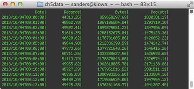
FIGURE 5.5 Data Throughput per Minute with Rwcount During Off-Peak Times
In the figure above you will notice that we see roughly 1.5 GB per minute traversing the sensor during off-peak hours at 00:00 UTC (which is 8 PM EST). However, if you look at the figure below (Figure 5.6) we see that traffic gets as high as 8-9 GB per minute during peak business hours at 17:00 UTC (which is 3 PM EST).
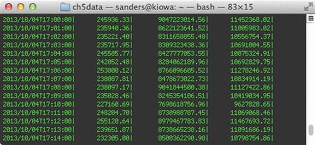
FIGURE 5.6 Throughput per Minute with Rwcount During Peak Times
To calculate an average throughput for the day, you can increase the bin-size in the rwcount command to count the total data for a single day, which is 86400 seconds.
cat daily.rw | rwcount --bin-size = 86400
Our results are shown in Figure 5.7.
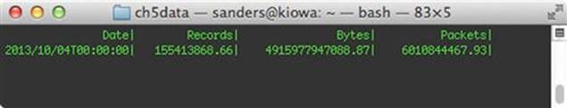
FIGURE 5.7 Calculating Average Throughput per Day
Using this calculation, we arrive at a total byte count of 4915977947088.87. We will want to get this number into something more manageable, so we can divide it by 1024 three times (4915977947088.87 × 1024− 3) to arrive at a total of 4578.36 GB. To arrive at the average throughput for this link on this day, we can take this byte count and divide it by the time quanta whose average we want to ascertain. This is 1440 minutes if you wish to have average number of bytes/minute, or 86400 seconds if you wish to have average number of bytes/second. This yields 3.18 GB bytes per minute (4578.36 / 1440) or 54.26 MB per second ((4578.36 / 86400) × 1024). While doing these calculations, all numbers were rounded to two places after the decimal point.
Decreasing the FPC Data Storage Burden
In an ideal world you could collect FPC data for every host, port, and protocol on your network and store it for a long time. In the real world, there are budgets and limitations that prevent that and sometimes we need to limit the amount of data we collect. Here we will talk about different strategies for eliminating the amount of FPC data you are retaining in order to get the best “bang for your buck” when it comes to data storage for NSM purposes.
Eliminating Services
The first and easiest method of paring down the amount of FPC data that is retained is to eliminate traffic generated by individual services. One way we can identify services that are a good fit for this strategy is to use rwstats, which can provide us with great detail on exactly how much the retention of data related to various ports, protocols, and hosts can affect your FPC data storage footprint. Rwstats is covered in extensive detail in Chapter 11, but we will go ahead and dive into it a bit here too. We will use two different rwstats commands to determine the ports associated with the largest volume of inbound and outbound traffic.
First, we’ll use rwstats to determine which ports are responsible for the most inbound communication within our example network. We will do that by calculating the source ports responsible for the most traffic, with this command:
cat daily.rw | rwstats --fields = sport --top --count = 5 --value = bytes
This command takes our original data set and feeds it to rwstats, which calculates the top 5 (--top --count = 5) source ports (--fields = sport) where the largest amount of data transfer occurred, by bytes (--value==bytes). The result is shown in Figure 5.8.
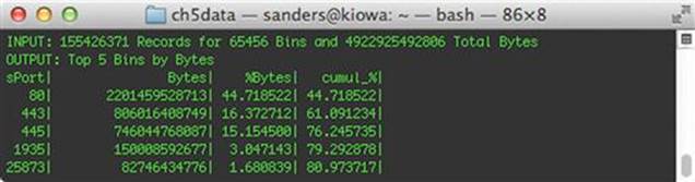
FIGURE 5.8 Top Communicating Source Ports
As you can see in the figure above, the majority of the traffic on this network segment is port 80 traffic, which we will assume is related to HTTP traffic. Specifically, 44% of the observed traffic is HTTP. Of course, HTTP traffic is immensely valuable for NSM detection and analysis so we probably want to keep this for now. However, if you look at the next line you will see that more than 16% of the total data transferred over the course of a day originated from source port 443. For the complete picture, let’s also take a look at the top 5 destination ports to get insight into outbound communication, using this command:
cat daily.rw | rwstats --fields = dport --top --count = 5 --value = bytes
The output from this command is shown in Figure 5.9.
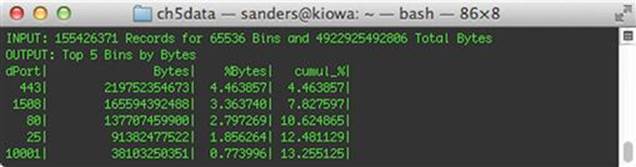
FIGURE 5.9 Top Communicating Destination Ports
The figure above shows that over 4% of traffic is destined to TCP/443, resulting in the conclusion that on a given business day, roughly 20.9% of all traffic traversing the monitoring interface of our sensor is TCP/443. Therefore, filtering out TCP/443 traffic will increase your total FPC data retention by 20.9% per business on average.
It is common for organizations to eliminate the collection of encrypted data that is a part of HTTPS communication. While the header information from encrypted data or statistics relating to it can be actionable, the encrypted data itself often isn’t. This is a good example of maximizing your FPC data storage by eliminating retention of data that doesn’t necessarily help you get the most bang for your buck when it comes to storage.
With TCP/443 traffic eliminated, we can revert back to our previous throughput calculation to see exactly how much of a dent it makes in those figures. We can modify our existing data set by using rwfilter to prune any TCP/443 traffic from our daily.rw file like this:
cat daily.rw | rwfilter --input-pipe = stdin --aport = 443 --fail = stdout| rwcount --bin-size = 86400
This command takes the existing daily.rw dataset and passes that data to another filter that will “fail out” any records that have port 443 as a source or destination address. That data is piped directly to rwcount to again present a statistic that shows total data traversing the sensor based on the new filter (Figure 5.10).
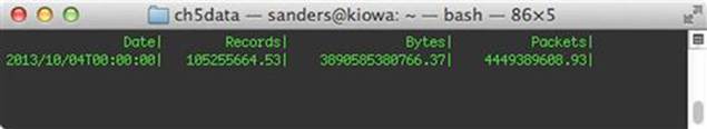
FIGURE 5.10 Throughput Statistics for the Same Day without TCP/443 Traffic
The figure above represents the exact same data as before, however this time with any TCP/443 traffic taken out. When we calculate the throughput values, we can see that this yields statistics of 2.52 GB per minute, or 42.9 MB per second. The result shows that removing TCP/443 traffic has indeed reduced the total amount of data that would be collected by ~ 20.9% during a business day.
This type of action can be taken for other ports containing encrypted data as well, such as ports used for encrypted VPN tunnels. While it might not be a good fit for every organization to consider, starting with removing encrypted data from FPC collection is just one example of how to reduce the burden of FPC data storage by eliminating the retention of traffic from specific services This also pays dividends later when it is time to parse FPC data for the creation of secondary data types during collection, as well as when parsing data for detection and analysis. Let’s look at some more ways that we can decrease the storage burden of FPC data.
Eliminating Host to Host Communication
Another way to reduce the amount of FPC data being stored is to eliminate the storage of communication between specific hosts.
Since we’ve already evaluated how much traffic will be reduced by dropping TCP/443 communication, let’s continue by removing that data from our next example. As you recall from earlier, we can “fail” anything that matches various criteria, so we will take advantage of that. In this example, we will look at the top-talking source and destination IP addresses remaining in the traffic after removing port 443 using this command:
cat daily.rw | rwfilter --input-pipe = stdin --aport = 443 --fail = stdout| rwstats --fields = sip,dip --top --count = 5 --value = bytes
This command sends our existing data set through another rwfilter command that removes any traffic matching TCP/443 on any port. This data is then piped to rwstats, which generates the top talking source and destination IP pairs (--fields = sip,dip) by the total amount of bytes transferred (--value = bytes). The result is shown in Figure 5.11.
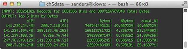
FIGURE 5.11 Identifying Top Talking IP Pairs
In the figure above we see that 19% of the communication on this network segment occurs between the hosts with the addresses 141.239.24.49 and 200.7.118.91. In order to determine whether this communication is a good candidate for exclusion from FPC data collection, you will have to dig a little deeper. Ideally, you would have friendly intelligence regarding the internal host you are responsible for, and would be able to identify the service that is responsible for this large amount of traffic. One way to do this with rwstats is to use the following query:
cat daily.rw | rwfilter --input-pipe = stdin --saddress = 141.239.24.49 --daddress = 200.7.118.91 --pass = stdout| rwstats --fields = sport --top --count = 10 --value = bytes
The results of this query are shown in Figure 5.12.
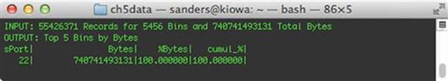
FIGURE 5.12 Examining Communication Between These Hosts
In this case, it looks like all of this communication is occurring on port 22. Assuming this is a legitimate connection, this probably means that some form of SSH VPN exists between these two devices. If you don’t have any ability to decrypt and monitor this traffic (such as through an intermediate proxy), then this would probably be a good candidate for exclusion from FPC data collection. This process can be repeated for other “top talkers” found on your network.
Using the strategies we’ve outlined here, we have successfully reduced the amount of FPC data being stored by around 40%. This means that your sensor can hold 40% more actionable data. Unfortunately, we can’t provide clear-cut examples of things that can be eliminated from FPC data storage in every network, because every network and every organization’s goals are so different. However, following the instructions provided in Chapter 2 for appropriately planning your data collection should help you make these determinations.
Caution
At the beginning of this chapter we mentioned that multiple other data types, such as PSTR, are often derived from FPC data. If your environment works in this manner, you should be aware of this when eliminating certain data types from FPC collection. For instance, if you generate PSTR data from FPC data and eliminate port 443 traffic, you won’t be able to generate packet strings from the HTTPS handshake, which will create a gap in network visibility. This might not be avoidable when space is limited, but if you still wish to keep this PSTR data you will have to find another way to generate it, such as doing so with another process directly from the wire.
Managing FPC Data Retention
Since FPC data eats up more disk space than any other data type per second, it is likely that it will be FPC data that causes your sensor to go belly up if data retention and rollover isn’t handled properly. I’ve seen even the most mature SOCs experience scenarios where a data spike occurs and it causes FPC data to be written to disk faster than it can be deleted. This can result in all sorts of bad things. Ideally, your FPC data storage exists on a volume that is separate from your operating system in order to prevent this from happening. However, even then I’ve even seen instances where FPC data was stored on shared dynamically expanding virtual storage, and a sustained spike in data led to other virtual devices being deprived of resources, ultimately leading to system crashes. There are dozens of other scenarios like this that can lead to the dreaded 2 AM phone call that nobody likes to make to systems administrators. With that in mind, this section is devoted to the management of FPC data; specifically, purging old data.
There are a number of ways to manage FPC data, but we will approach this from a simple perspective that only uses tools built in to most Linux distributions. This is because these tools are effective, and can be scripted easily. While some of the techniques we describe in this section might not fit your environment perfectly, we have confidence that they can be adapted fairly easily.
Earlier, we discussed the two most common strategies that organizations use for storing FPC data: time-based and size-based. The method for managing these two strategies varies.
Time-Based Retention Management
Using a time-based retention strategy is fairly easy to manage in an automated fashion. The linux find utility can easily search for files with modify times that are of a certain age. For instance, in order to find files older than 60 minutes within the /data/pcap/ directory, simply run the following command;
find /data/pcap -type f -mtime + 60
From that command you can generate a file list of PCAPs that you wish to delete. This command can be modified by pairing it with xargs in order to remove data that meets this criteria. The following one-liner will remove any data older than 60 minutes.
find /data/pcap -type f -mtime + 60 | xargs -i rm {}
Size-based Retention Management
Managing FPC data that is using a size-based retention strategy is a bit more difficult. This method of data retention deletes the oldest PCAP files once the storage volume exceeds a set percentage of utilized disk space. Depending on your FPC collection deployment, this method can be challenging to implement. If you are able to use Daemonlogger, it has the capability to do this type of data purging on its own, as was described earlier. If you are using a tool that doesn’t have this feature built in, purging data in this manner requires a bit more critical thinking.
One way to handle this is through a BASH script. We’ve provided such a script here:
#!/bin/bash
## This script deletes excess PCAP when the “percentfull” reaches the predefined limit.
## Excess PCAP is when the total amount of data within a particular PCAP directory
## reaches the percent amount defined about, out of the total amount of drive space
## on the drive that it occupies. For the purpose of consistency, the percentfull amount
## is uniform across all PCAP data sources.
## Refer to the “Data Removal Configuration (DRC)” at the bottom of this script for settings.
#Example DRC;
## Data Removal Configuration
#dir = “/data/pcap/eth1/”
#percentage = 1
#datamanage $dir $percentage
#dir = “/data/pcap/eth2/”
#percentage = 3
#datamanage $dir $percentage
##################################################################
## FUNCTION #######################################################
##################################################################
totaldiskspace = $(df | grep SOsensor-root | awk '{print $2}')
function datamanage {
# Initial data evaluation
datadirectory = “$1”
datapercent = “$2”
datasize = $(du -s $datadirectory | awk '{print $1}')
diskstatus = $(df | grep SOsensor-root | awk '{print $5}' | egrep -o '[0-9]{1,3}')
datapercentusage = $(echo “scale = 2; $datasize / $totaldiskspace * 100” | bc | sed 's/\..*//g')
echo “Data usage in $datadirectory is at $datapercentusage% of hard drive capacity)”
# Data Removal Procedure
while [ “$datapercentusage” -gt “$datapercent” ]; do
filestodelete = $(ls -tr1 $datadirectory | head -20)
printf %s “$filestodelete” | while IFS = read -r ifile
do
echo $ifile
if [ -z $datadirectory$ifile ]; then
exit
fi
echo “Data usage in $data directory ($datapercentusage%) is greater than your desired amount ($datapercent% of hard drive)”
echo “Removing $datadirectory$ifile”
sudo rm -rf $datadirectory$ifile
du -s $datadirectory
# datasize = $(du -s $datadirectory | awk '{print $1}')
done
datasize = $(du -s $datadirectory | awk '{print $1}')
datapercentusage = $(echo “scale = 2; $datasize / $totaldiskspace * 100” | bc | sed 's/\..*//g')
du -s $datadirectory
datasize = $(du -s $datadirectory | awk '{print $1}')
datapercentusage = $(echo “scale = 2; $datasize / $totaldiskspace * 100” | bc | sed 's/\..*//g')
done
}
# Data Removal Configuration
pidofdiskclean = $(ps aux | grep diskclean.sh | wc -l)
echo $pidofdiskclean
if [ “$pidofdiskclean” -le “4” ]; then
dir = “/data/pcap/eth1/”
percentage = 40
datamanage $dir $percentage
dir = “/data/pcap/eth2/”
percentage = 40
datamanage $dir $percentage
wait
echo “”
fi
To use the script above you must configure the volume name where data is stored by editing the dir variable. Additionally, you must configure the Data Removal Configuration section near the bottom of the script to indicate the directories where PCAP data is stored, and the amount of empty buffer space you wish to allow on the volume.
The script will take these variables and determine the percentage of utilized space that is taken up by the data within it. If it determines that this percentage is above the allowable amount, it will remove the oldest files until the percentage is at a suitable level.
This script can be placed in a scheduled cron job that runs on a regular basis, such as every hour, every 10 minutes, or every 60 seconds. How frequently it runs will depend on how much of an empty space buffer you allow, and how much throughput you have. For instance, if you only leave 5% of empty buffer space and have a large amount of throughput, you will want to ensure the script runs almost constantly to ensure that data spikes don’t cause the drive to fill up. On the flip side, if you allow 30% of empty buffer space and the link you’re monitoring has very little throughput, you might be fine only running this script every hour or so.
In a scenario where your sensor is under a high load and empty buffer space is very limited, your cron job has a chance of not running in time to remove the oldest files. However, if you run the script constantly, for instance on a sleep timer, you can still run the risk of slower script performance in calculating disk space requirements during execution. To split the difference, it is often ideal to require the script to calculate disk space, determine if the directory is too full, and then delete the 10 oldest files, instead of just the individual oldest file. This will increase script performance dramatically, but can result in less than maximum retention (but not by much). The script below will perform that task in a manner similar to the first script we looked at.
#!/bin/bash
## This script deletes excess pcap when the “percentfull” reaches the predefined limit.
## Excess pcap is when the total amount of data within a particular pcap directory
## reaches the percent amount defined about, out of the total amount of drive space
## on the drive that it occupies. For the purpose of consistency, the percentful amount
## is uniform across all pcap data sources.
## Refer to the “Data Removal Configuration (DRC)” at the bottom of this script for settings.
#Example DRC;
## Data Removal Configuration
#dir = “/data/pcap/eth6/”
#percentage = 1
#datamanage $dir $percentage
#dir = “/data/pcap/eth7/”
#percentage = 3
#datamanage $dir $percentage
##################################################################
## FUNCTION #######################################################
##################################################################
totaldiskspace = $(df | grep SOsensor-root | awk '{print $2}')
function datamanage {
# Initial data evaluation
datadirectory = “$1”
datapercent = “$2”
datasize = $(du -s $datadirectory | awk '{print $1}')
diskstatus = $(df | grep SOsensor-root | awk '{print $5}' | egrep -o '[0-9]{1,3}')
datapercentusage = $(echo “scale = 2; $datasize / $totaldiskspace * 100” | bc | sed 's/\..*//g')
echo “Data usage in $datadirectory is at $datapercentusage% of hard drive capacity)”
# Data Removal Procedure
while [ “$datapercentusage” -gt “$datapercent” ]; do
filestodelete = $(ls -tr1 $datadirectory | head -10)
echo $filestodelete
printf %s “$filestodelete” | while IFS = read -r ifile
do
echo $ifile
if [ -z $datadirectory$ifile ]; then
exit
fi
echo “Data usage in $datadirectory ($datapercentusage%) is greater than your desired amount ($datapercent% of hard drive)”
echo “Removing $datadirectory$ifile”
sudo rm -rf $datadirectory$ifile
done
datasize = $(du -s $datadirectory | awk '{print $1}')
datapercentusage = $(echo “scale = 2; $datasize / $totaldiskspace * 100” | bc | sed 's/\..*//g')
done
}
# Data Removal Configuration
pidofdiskclean = $(ps aux | grep diskclean.sh | wc -l)
echo $pidofdiskclean
if [ “$pidofdiskclean” -le “4” ]; then
# Data Removal Configuration
dir = '/data/pcap/eth1/'
percentage = 10
datamanage $dir $percentage
dir = “/data/pcap/eth2/”
percentage = 10
datamanage $dir $percentage
wait
fi
While the code samples provided in this section might not plug directly into your environment and work perfectly, they certainly provide a foundation that will allow you to tweak them for your specific collection scenario. As another resource, consider examining the scripts that Security Onion uses to manage the retention of packet data. These scripts use similar techniques, but are orchestrated in a slightly different manner.
Conclusion
FPC data is the most thorough and complete representation of network data that can be collected. As a primary data type, it is immensely useful by itself. However, its usefulness is compounded when you consider that so many other data types can be derived from it. In this chapter we examined different technologies that can be used for collecting and storing FPC data. We also discussed different techniques for collecting FPC data efficiently, paring down the amount of FPC data you are collecting, and methods for purging old data. As we move on through the remainder of the collection portion of this book, you will see how other data types can be derived from FPC data.
All materials on the site are licensed Creative Commons Attribution-Sharealike 3.0 Unported CC BY-SA 3.0 & GNU Free Documentation License (GFDL)
If you are the copyright holder of any material contained on our site and intend to remove it, please contact our site administrator for approval.
© 2016-2026 All site design rights belong to S.Y.A.