Blender For Dummies (2015)
Part III
Get Animated
 Visit www.dummies.com/extras/blender for great Dummies content online.
In this part . . .
· Constraining objects.
· Using shape keys, hooks, and armatures.
· Applying the Dope Sheet.
· Simulating physics.
· Visit www.dummies.com/extras/blender for great Dummies content online.
Chapter 10
Animating Objects
In This Chapter
![]() Using the Graph Editor
Using the Graph Editor
![]() Putting constraints on objects and taking advantage of these constraints
Putting constraints on objects and taking advantage of these constraints
![]() Practicing with animation
Practicing with animation
I have to make a small admission: Animation is not easy. It's time consuming, frustrating, tedious work where you often spend days, sometimes even weeks, working on what ends up to be a few seconds of finished animation. An enormous amount of work goes into animation. However, there's something incredible about making an otherwise inanimate object move, tell a story, and communicate to an audience. Getting those moments when you have beautifully believable motion — life, in some ways — is a positively indescribable sensation that is, well, indescribably positive. Animation, and the process of creating animation, truly has my heart more than any other art form. It's simply my favorite thing to do. It's like playing with a sock puppet, except better because you don't have to worry about wondering whether or not it's been washed.
This chapter, as well as the following three chapters, go pretty heavily into the technical details of creating animations using Blender. Blender is a great tool for the job. Beyond what this book can provide you with, though, animation is about seeing, understanding, and re-creating motion. I highly recommend that you make it a point to get out and watch things. And not just animations: Go to a park and study how people move. Try to move like other people move so that you can understand how the weight shifts and how gravity and inertia compete with and accentuate that movement. Watch lots of movies and television and pay close attention to how people's facial expressions can convey what they're trying to say. If you get a chance, go to a theater and watch a play. Understanding how and why stage actors exaggerate their body language is incredibly useful information for an animator.
 While you're doing that, think about how you can use the technical information in these chapters to re-create those feelings and that motion with your objects in Blender.
Working with Animation Curves
In Blender, the fundamental way for controlling and creating animation is with animation curves called f-curves. F-curve is short for function curve, and it describes the change, or interpolation, between two key moments in an animated sequence.
To understand interpolation better, flash back to your grade-school math class for a second. Remember when you had to do graphing, or take the equation for some sort of line or curve and draw it out on paper? By drawing that line, you were interpolating between points. Don't worry though; I'm not going to make you do any of that. That's what we have Blender for. In fact, the following example shows the basic process of animating in Blender and should help explain things more clearly:
1. Start with Blender's default scene (Ctrl+N⇒Reload Start-Up File).
2. Select the default cube object and switch to the camera view (right-click, Numpad 0).
3. Split the 3D View horizontally and change one of the new areas to the Graph Editor (Shift+F6).
 I like to make the lower one the Graph Editor, because it's right above the Timeline in the default screen layout.
4. In the 3D View, make sure that the default cube is selected and press I⇒Location.
This step sets an initial location keyframe for the cube. I give a more detailed description of keyframes later in the chapter in the “Inserting keys” section. The important thing to notice is that the left region of the Graph Editor is now updated and shows a short tiered list with the items Cube, CubeAction, and Location.
5. Press Shift+↑ on your keyboard.
You move forward in time by 10 frames.
6. Grab (G) the cube in the 3D View and move it to another location in the scene.
7. Press I⇒Location again in the 3D View. A set of colored lines appears in the Graph Editor. These colored lines are f-curves. Each f-curve represents a single attribute, or channel, that's been animated. If you expand the Location block in the Graph Editor by left-clicking the triangle on the left side of its name, you can see the three location channels: X Location, Y Location, and Z Location. To see the actual curves a little bit better, move your mouse to the large graph section of the Graph Editor and press Home. Your Blender screen should look something like the one in Figure 10-1.
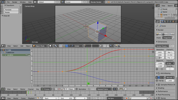
Figure 10-1: Animating the location of the default cube object.
Congratulations! You just created your first animation in Blender. Here's what you did: The largest part of the Graph Editor is a graph (go figure!). Moving from left to right on this graph — its X-axis — is moving forward in time. The vertical axis on this graph represents the value of whatever channel is being animated. So the curves that you created describe and control the change in the cube's location in the X-, Y-, and Z-axes as you move forward in time. Blender creates the curves by interpolating between the control points, called keys, that you created.
You can see the result for yourself by playing back the animation. Keeping your mouse cursor in the Graph Editor, press Alt+A (alternatively, you can left-click the Play button in the Timeline). A green vertical line, called the timeline cursor, moves from left to right in the graph. As the timeline cursor moves, you should see your cube move from the starting point to the ending point you defined in the 3D View. Press Esc to stop the playback. You can watch the animation in a more controlled way by scrubbing in the Graph Editor. To scrub, left-click in the graph area of the Graph Editor and drag your mouse cursor left and right. The timeline cursor follows the location of your mouse pointer, and you can watch the change happening in the 3D View.
Customizing your screen layout for animation
There is a screen layout in Blender specifically set up for animation named — conveniently — Animation. You can choose it from the Screen Layout datablock in the Info editor at the top of the Blender window or by using the Ctrl+ ← ⇒ Ctrl + ← hotkey combination.
This screen layout isn't too dissimilar from the Default layout, but it does have a few differences. In particular, the Outliner is larger, and on the left side of the screen, there's a Dope Sheet and Graph Editor. A second 3D View is also placed above the Outliner. The Timeline from the Default layout is pretty much unchanged. (For a full reminder of what each editor does, refer to Chapter 1.)
You may be wondering, however, why this layout has three editors (the Timeline, Graph Editor, and Dope Sheet) that allow you to adjust your position in time on your animation. The quick answer is that each editor gives you different kinds of control over your animation. For example, the Timeline gives you a central place to control the playback of your overall animation. This way, you can use the Graph Editor to focus on specific detailed animations and the Dope Sheet for making sense of complex animation with a lot of animated attributes. Like the Graph Editor, you can scrub the Timeline and Dope Sheet by left-clicking in it and dragging your mouse cursor left and right.
One change I usually like to make to this layout is in the secondary 3D View above the Outliner. I like to change the viewport shading in this editor to be Shaded (Z) or Textured (Alt+Z). The reason for this secondary view is so that you can work from any perspective in the main 3D View but still retain an idea of what the camera sees. That way, you don't end up animating something that will never be on camera. The default Wireframe shading in this 3D View is good for fast playback, but it's usually too difficult to tell what's going on. I also like to disable the 3D Manipulator (Ctrl+Spacebar) in that secondary 3D View so it doesn't get in the way of seeing the actual animation.
To that end, I also use Blender's Only Render display. Only Render hides anything that won't be rendered (3D grid, relationship lines, lamps, empties, and so on) from the 3D View, allowing you to get a truer understanding of what your final animation looks like. To activate this feature, reveal the Properties region (N) in this secondary 3D View and enable the Only Render check box in the Display panel.
The last change I make to this screen layout is in the main 3D View. I swap out the Translate manipulator for the Rotate manipulator (if you have the Pie Menus add-on enabled, you can do this quickly by using Ctrl+Spacebar ⇒ Rotate) and change its coordinate space to Normal (Alt+Spacebar ⇒ Normal). I do this change because normally I can grab and scale with the G and S hotkeys pretty quickly, but precise rotation when animating is often faster and easier with the Rotate manipulator. Plus, this manipulator doesn't obstruct my view as much as the other ones do. Figure 10-2 shows my modestly modified Animation screen layout.
Figure 10-2: The Animation screen layout with a few small modifications to make working more pleasant.
Working in the Graph Editor
Working in the Graph Editor is very similar to working in the 3D View. The following describes the basic controls available in the Graph Editor:
· Middle-click+drag moves around your view of the graph.
· Ctrl+middle-click+drag allows you to interactively scale your view of the curve horizontally and vertically at the same time.
· Scroll your mouse wheel to zoom in and out.
· Shift+scroll moves the graph vertically.
· Ctrl+scroll moves the graph horizontally.
· Right-click selects individual f-curve control points.
· Press A to toggle selecting all or no control points.
· Press B for Border Select.
· Press N to reveal the Graph Editor's Properties region (similar to the Properties region in the 3D View).
· Left-click a channel in the left region of the Graph Editor to select it.
You may need to expand the blocks in this region to drill down to the actual animation channels (such as X Location, Y Location, and Z Location).
· Ctrl+left-click allows you to arbitrarily add points to a selected f-curve in the graph. Anywhere you Ctrl+left-click in the graph, a new control point is added to the selected channel.
The Graph Editor also has some handy keyboard shortcuts for hiding and revealing channels. They're particularly useful when you want to manage a complex animation with a lot of keyframes and channels. If you select one or more keyframes, you can use any of these hotkeys:
· H hides the channels that the selected keyframes belong to.
· Shift+H hides all channels except for the ones where you've selected a keyframe.
· Alt+H reveals (“unhides”) all animation channels in the Graph Editor.
Inserting keys
Instead of Ctrl+left-clicking in the Graph Editor to add control points to a specific f-curve, you have another, more controlled option. Blender also uses a workflow that's a lot more like traditional hand-drawn animation. In traditional animation, a whole animated sequence is planned out ahead of time using a script and storyboards (drawings of the major scenes of the animation, kind of like a comic book, with arrows to indicate camera direction). Then an animator goes through and draws the primary poses of the character. These drawings are referred to as keyframes or keys. They're the poses that the character must make in order to most effectively convey the intended motion to the viewer. With the keys drawn, they’re handed off to a second set of animators called the inbetweeners. These animators are responsible for drawing all the frames between each of the keys in order to get the appearance of smooth motion.
Creating the illusion of motion with static images
In order to effectively do animation, you really need a firm grasp on how moving pictures work. This is the fundamental basis of animation, and film, television, and even video games. Without getting into the complex details of psychology and neuroscience, the basics are this: humans perceive movement as the apparent difference in what we see at two relatively close moments in time.
If you have two images of the same object in different positions, you can create the illusion that the object moves between positions by swapping between those images very quickly. Now chain a series of those images together and show them in quick succession. Each image is only visible for a fraction of a second before the next one appears. This rapid swapping of images tricks our minds into seeing movement on the screen.
Who said science isn't fun?
Translating the workflow of traditional animation to how you do work in Blender, you should consider yourself the keyframe artist and Blender the inbetweener (at least to start). On a fully polished animation, it isn't uncommon to have some kind of key on every frame of animation. In the quick animating example at the beginning of this section, you create a keyframe after you move the cube. By interpolating the curve between those keys, Blender creates the in-between frames. Some animation programs refer to creating these in-between frames as tweening.
To have a workflow that's even more similar to traditional animation, it’s preferable to define your keyframes in the 3D View. Then you can use the Graph Editor to tweak the change from one keyframe to the next. And this workflow is exactly the way Blender is designed to animate. Start in the 3D View by pressing I to bring up the Insert Keyframe menu. Through this menu, you can create keyframes for the main animatable channels for an object. I describe the channels here in more detail:
· Location: Insert a key for the object's X, Y, and Z location.
· Rotation: Insert a key for the object's rotation in the X, Y, and Z axes.
· Scaling: Insert a key for the object's scale in the X, Y, and Z axes.
· LocRot/LocScale/LocRotScale/RotScale: Insert keyframes for various combinations of the previous three values.
· Visual Location/Rotation/LocRot: Insert keyframes for location, rotation, or both, but based on where the object is visually located in the scene. These options are explicitly made for use with constraints, which I cover later in this chapter in “Using Constraints Effectively.”
· Available: If you already inserted keys for some of your object's channels, choosing this option adds a key for each of those preexisting curves in the Graph Editor. If no curves are already created, no keyframes are inserted.
· Delta Location/Rotation/Scale: With the exception of Available, all of the preceding keying options use absolute coordinates for keying animations. Delta keys, however, use coordinates relative to your object's current location, rotation, and scale. Delta keys can be useful if you want to have many objects with the same animation, but starting from different origin points.
When Blender sets keyframes for location, rotation, and scale, bear in mind which coordinate system the Graph Editor is using. Location is stored in global coordinates, whereas rotation and scale are stored in the object's local coordinate system.
Here’s the basic workflow for animating in Blender:
1. Insert an initial keyframe (I).
A keyframe appears at frame 1 in your animation. Assuming that you enter a Location keyframe, if you look at the Graph Editor, notice that Location channel is added and enabled.
2. Move forward 10 frames (Shift+↑).
This puts you at frame 11. (Of course, when doing a real animation, your keys aren't always going to be 10 frames apart.) The Shift+↑ and Shift+↓ hotkeys move you 10 frames forward or backward in time, regardless of the editor your mouse cursor is in.
This is a good way to rough in your keys. You can go back later and adjust your timing from the Dope Sheet or Graph Editor. To move forward or back one frame at a time, use the ← and → keys. Of course, you can also use the Timeline, Graph Editor, or Dope Sheet to change what frame you are in.
3. Grab your cube and move it to a different location in 3D space (G).
4. Insert a new keyframe (I).
Now you should have curves in the Graph Editor that describe the motion of the cube.
You can insert keys in an easier way using a feature called Autokey. Like its name indicates, Autokey automatically creates keys when you make changes in your scene. To enable the Autokey feature, look in the Timeline. Next to the playback controls in the Timeline's header is a button with a red circle on it, like the Record button on a DVR. Left-click it to activate Autokey. Now you can simply use tools in the 3D View like grab (G), rotate (R), and scale (S) as you move forward in time and keyframes are automatically inserted for you. Pretty sweet, huh?
By default, Blender uses the LocRotScale keying set (there's more on keying sets later in this chapter) for inserting keyframes when Autokey is enabled. This is worth noting because, if you're not careful, Autokey can insert keyframes that are unnecessary or (worse) not wanted. It's for this reason that when I use Autokey, I like to insert my initial keyframes manually and then use the Available keying set for autokeying.
A really cool feature in Blender is the concept of “[almost] everything animatable.” You can animate nearly every setting or attribute within Blender. Want to animate the skin material of your character so that she turns red with anger? You can! Want to animate the Count attribute in an Array modifier to dynamically add links to a chain? You can! Want to animate whether your object appears in wireframe or solid shading in the 3D View? Ridiculous as it sounds, that, too, is possible!
So how do you do this miraculous act of animating any attribute? It's amazingly simple. Nearly every text field, value field, color swatch, drop-down menu, check box, and radio button is considered a property and represents a channel that you can animate. Insert a keyframe for that channel by right-clicking one of those properties and choosing Insert Keyframes from the menu that appears. Figure 10-3 shows what this menu looks like.
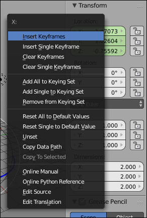
Figure 10-3: Right-click any property in the Properties editor, and you can insert a keyframe for it.
After you insert a new keyframe for that property, its color changes to yellow, and a channel for that property is added in the Graph Editor. When you move forward or backward in time, the color of the control changes from yellow to green. This green color indicates that the property is animated, but you're not currently on one of its keys. Insert another keyframe for that property, and BAM! The field's color turns to yellow and you have two keyframes for your animated property.
For an even faster way to insert keyframes on properties, hover your mouse over the control and just press I. This trick even works on the show/hide/selectable icons (known as the restrict columns) in the Outliner. How's that for awesome?
If you want to insert keyframes on multiple properties at the same time (such as the aforementioned restricted columns in the Outliner), keep holding the I hotkey as you run your mouse cursor over those properties. There you go. One key press, many keyframes.
Working with keying sets
When working on an animation, you can easily find yourself inserting keyframes for a bunch of different channels and properties at the same time. The troublesome thing is that, on a complex scene, these properties can be located all over Blender's interface. Sure, you can insert keys for an object's location, rotation, and scale by pressing I in the 3D View, but you may also need to key that object's visibility from the Outliner, the influence of a constraint in Constraint Properties, and the object's material color from Material Properties. They're all over the place! It wouldn't be difficult at all to overlook one while you work, resulting in an animation that doesn't quite behave the way you want it to.
This load can be lightened by using more advanced rigging features (see Chapter 11), but even that doesn't really solve it. A complex character rig can have hundreds of bones and controls to animate. Manually keeping track of all of them for multiple characters in a scene can be a nightmare. (I know. I've tried.)
You know what would be really nice? It would be great if you could make a custom group of a bunch of properties so you can insert a keyframe for all of them at the same time, kind of like the LocRotScale option when you press I in the 3D View. Well, guess what? That exact feature exists in Blender. It's called a keying set.
 Actually, the LocRotScale option is a keying set. It's one of a handful of pre-configured keying sets that ship with Blender. In fact, all of the options in the Insert Keyframe Menu (I) are keying sets.
Using keying sets
To use keying sets, start with a look at the last set of fields and buttons of the Timeline's header, just to the right of the Autokey button, as shown in Figure 10-4.

Figure 10-4: The Timeline's header has controls for choosing your active keying set and inserting keyframes within that keying set.
There are three widgets in the Timeline for working with keying sets:
· Active keying set: This field for this drop-down menu is empty by default. Left-click on it to choose one of the available keying sets to be your active one.
If you have an active keying set, you can make this field empty again by left-clicking the X to the right of your keying set's name.
· Insert keyframes: Left-click this button to insert a keyframe at the current frame on the Timeline for every property in the current active keying set. If you don't have an active keying set, a little error pops up to let you know.
· Remove keyframes: Left-click this button to remove any keyframes from the current frame that belong to any properties in the active keying set.
If you don't have any keys on the current frame, this button doesn't do anything.
To quickly choose an active keying set from the 3D View, use the Ctrl+Shift+Alt+I hotkey combination.
When you choose a keying set, Blender gives preference to the properties in that keying set when you insert keyframes. This means that with an active keying set chosen, you don't get the Insert Keyframe menu if you press I in the 3D View. Blender just quietly inserts keyframes for all of the properties in your chosen keying set. This lack of immediate feedback may be disorienting at first, but it makes for a very fast, distraction-free workflow for animating. Also, as mentioned earlier in this chapter, if you have Autokey enabled, it uses the active keying set. If you don't have an active keying set chosen, Autokey defaults to using the LocRotScale keying set.
Creating custom keying sets
The pre-configured keying sets that come with Blender are handy, but it's much more useful to define your own keying sets (especially as your animations become more complex). Keying sets aren't character or object-specific, so they apply to your whole scene. This means you can use a keying set to insert keyframes for a whole group of characters all at the same time if you like.
Because keying sets are relevant to your whole scene, you can create your custom keying sets from Scene Properties, in the Keying Sets panel. Follow these steps to create a new keying set and populate it with properties to keyframe:
1. In the Keying Sets panel, left-click the Plus (+) button to the right of the keying set list box.
2. Adjust your new keying set's settings.
Double-click its name in the listbox to rename it to something other than the generic Keying Set that you get by default. You can use the Description text field to write a few words that explain the purpose of your custom keying set.
On the bottom right of the panel, there are three toggleable settings that you can choose to enable or disable:
· Only Needed: Enable this option, and Blender only adds keyframes to the properties that changed since the last inserted keyframe. If the property didn't change, no keyframe is inserted, regardless of whether you've pressed I in the 3D View.
· Visual Keying: As covered earlier in this chapter, visual transforms the location, rotation, and scale of your object as they appear on-screen, including changes made by constraints. Enable this option and all inserted keyframes in this keying set will use visual transforms for keying.
· XYZ=RGB Colors: This option is enabled by default. It dictates that any new f-curves use red, green, and blue for X-, Y-, and Z-axis channels.
The buttons for the Keyframing Settings are configured in the Blender interface as radio buttons (if you left-click one to enable it, the others are automatically disabled). You can enable two or more of these settings by Shift+left-clicking them.
Figure 10-5 shows the Keying Sets panel with a few custom keying sets added in the list box.
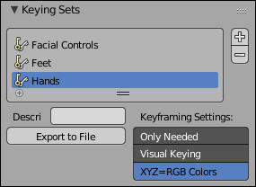
Figure 10-5: The Keying Sets panel is where you add new custom keying sets.
Left-clicking a keying set in the list box of the Keying Sets panel automatically makes that keying set the active one.
At this point, you've created your custom keying set, but it starts as an empty container. You haven't assigned any properties to it. To add, edit, and remove properties from your active keying set, you need to use the Active Keying Set panel in Scene Properties. It appears below the Keying Sets panel when you have a custom keying set selected in the list box.
To add a new property to your custom keying set, you need to tell Blender where to find that property. You need to give Blender that property's path, or the way to navigate through your .blend file's internal structure to your property. It's certainly possible (and sometimes necessary for more obscure properties) to manually add new paths from the Active Keying Set panel by left-clicking the Plus (+) button next to the Paths list box and get more specific from there. However, that can be an excruciatingly tedious process, even if you have a strong working knowledge of .blend file innards.
There's a better, easier way to populate your keying set. Rather than go about the painful, manual way, follow these steps:
1. In Blender's interface, find the property you want to add to your keying set.
This could be the material color of your object, just its Y-axis rotation, or its renderability in the Outliner. It can be any property that's capable of being keyframed.
2. Right-click the field or button or check box for that property.
Among all of the various options that are available in the menu that appears, there should be either two or three menu items that are specific to keying sets:
· Add All to Keying Set: If your chosen property is one of a block of properties (such as X, Y, and Z scale), this option can add all of the properties in that block to your custom keying set. If the property isn't part of such a block, this option doesn't appear in the menu.
· Add Single to Keying Set: Choose this option to add just the property that you've right-clicked to your keying set.
If the property isn't part of a block of properties, then this menu item reads as Add to Keying Set.
· Remove from Keying Set: If the property in question already is in your active keying set, you can choose this option to quickly remove it.
3. Add the property to your active keying set by left-clicking one of the Add to Keying Set menu items.
Your chosen property is now a member of the active keying set. You can verify that it's there by looking at the Paths list box in the Active Keying Set panel of Scene Properties. Figure 10-6 shows the Active Keying Set panel with a few paths added.
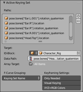
Figure 10-6: The properties of your active keying set are listed in the Active Keying Set panel of Scene Properties.
You may notice in Figure 10-6 that, like the Keying Sets panel, the Active Keying Set panel features the same three buttons for Keyframing Settings. By adjusting these settings in the Active Keying Set panel, you override the global Keyframing Settings as defined in the Keying Sets panel, but just for that property.
 The override behavior in the Active Keying Set panel only works in an additive way. That is, if you have Only Needed disabled in the Keying Sets panel, enabling it for a specific property in the Active Keying Set panel will override as expected. However, if that same option is enabled in the Keying Sets panel, currently there isn't a clean way to do an override that disables it for individual properties in the keying set.
To the left of the Keyframing Settings is a drop-down menu labeled F-Curve Grouping. This drop-down menu dictates how animation channels are grouped in the Dope Sheet and Graph Editor. You have three choices:
· Keying Set Name: This is the default setting. Animation channels in the Dope Sheet and Graph Editor are grouped according to the name of your keying set.
It generally works well, but if you have a lot of properties in your keying set, this can make that grouping seem a bit like a grab bag of animated properties.
· None: You have the option of not grouping the properties in your keying set at all. This can lead to pretty messy animation editors, so it isn't an option you'll choose often, but it's nice to know it's available.
· Named Group: This is a very powerful option for organizing a large keying set. If you choose Named Group as your method for f-curve grouping, a text field labeled Group appears below the drop-down menu. Type the name of a group in that field. Now, if you choose another property in your keying set and type the exact same group name, both properties are collected together in the Dope Sheet and Graph Editor. As covered in Chapter 11, this is extremely useful for complex character rigs.
Editing motion curves
After you know how to add keyframes to your scene, the next logical step is to tweak, edit, and modify those keyframes, as well as the interpolation between them, in the Graph Editor. The Graph Editor is similar to the 3D View, and you can select individual control points on f-curves by right-clicking or by pressing B for Border Select or even by pressing C for circle selection. Well, the similarities with the 3D View goes farther than that. Not only can you select those control points in the Graph Editor, but you can edit them like a 2D Bézier curve object in the 3D View. The only constraint is that f-curves can’t cross themselves. Having a curve that describes motion in time do a loopty-loop doesn't make any sense.
For more detailed descriptions of the hotkeys and controls for editing Bézier curves in Blender, see Chapter 6. Selecting and moving control point handles, as well as the V hotkey for changing handle types all work as expected. However, because these curves are specially purposed for animation, you have a few additional controls over them. For example, you can control the type of interpolation between control points on a selected curve by pressing T or going to Key ⇒ Interpolation Mode in the Graph Editor's header. You get the following options:
· Interpolation: These three options control the general interpolation between two keyframes.
· Constant: This option is sometimes called a step function because a series of them look like stair steps. Basically, this interpolation type keeps the value of one control point until it gets to the next one, where it instantly changes. Many animators like to use this interpolation mode when blocking out their animations. This way, they can focus on getting their poses and timing right without the distraction of in-between frames.
· Linear: The interpolation from one control point to the next is an absolutely straight line. This option is similar to changing two control points to have Vector handles.
· Bézier: The default interpolation type, Bézier interpolation smoothly transitions from one control point to the next. In traditional animation, this smooth transition is referred to as easing in and easing out of a keyframe.
· Easing (by strength): The interpolation options in this column are preset, “mathematically correct” interpolation methods. You can get the same curve profile by manually editing the handles of a curve with Bézier interpolation, but these easing presets are a faster way of getting the same result.
· Dynamic Effects: When things move in meatspace, there isn't always a smooth transition from one pose to the next. When you drop a ball to the ground, it bounces. When you slam on the brakes while driving, the car over-extends, lurching forward before settling back to rest. In many cases, you can (and should) animate this behavior by hand. However, in a pinch, these three Dynamic Effects interpolation can give you a great starting point:
· Back: In this interpolation type, the curve “overshoots the mark” set by the keyframe before settling back where you want it. To see what this effect is like, try slapping the surface of a table, but stopping just before your hand makes contact. If you watch carefully, you should notice that your hand goes a bit farther than you want it to before it finishes moving.
· Bounce: The Bounce interpolation is a fun one. It makes your object appear to bounce before coming to a rest.
· Elastic: Have you ever seen an over-extended rubber band break in half? The loose ends flop all over the place before they stop moving. The Elastic interpolation mode gives your object this kind of effect, like it's stuck to the floppy end of one of those broken rubber bands.
Figure 10-7 shows the Keyframe Interpolation menu.
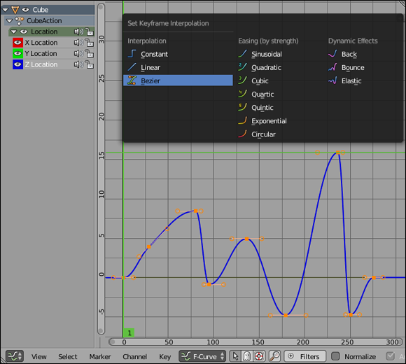
Figure 10-7: Changing the interpolation type on selected f-curve control points.
The interpolation mode options work only on the selected control points in the Graph Editor, so if you want to select all the control points in a single f-curve, select one of those control points and press L. Then you can apply your interpolation mode to the entire curve.
You can also change what a selected f-curve does before and after its first and last keyframes by changing the curve's extrapolation mode. You can change a curve's extrapolation mode by selecting an f-curve channel in the left region of the Graph Editor and then pressing Shift+E or navigating to Key ⇒ Extrapolation Mode in the Graph Editor's header. When you do, notice four possible choices:
· Constant Extrapolation: This setting is the default. The first and last control point values are maintained into infinity beyond those points.
· Linear Extrapolation: Instead of maintaining the same value in perpetuity before and after the first and last control points, this extrapolation mode takes the directions of the curve as it reaches those control points and continues to extend the curve in those directions.
· Make Cyclic (F-Modifier): This option adds an f-curve modifier (covered in the next section of this chapter) that takes all of the keyframes in your animation and repeats them before and after your first and last keyframes.
If you have a looping animation, like a character who never stops waving at you, this option is an easy way to make that happen.
· Clear Cyclic (F-Modifier): If your f-curve has a Cycles modifier, it's possible to remove that modifier from the Graph Editor's Properties region (N), but this menu option is faster.
Figure 10-8 shows the menu for the different type of extrapolation modes, as well as what each one looks like with a simple f-curve.
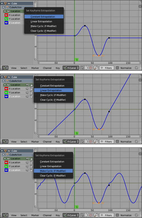
Figure 10-8: The four extrapolation modes you can have on f-curves.
If you have lots of animated objects in your scene, or just one object with a high number of animated properties, it may be helpful to hide extraneous curves from view so that you can focus on the ones you truly want to edit. To toggle a curve's visibility (or that of an entire keying set), left-click the eye icon next to its name in the channel region along the left side of the Graph Editor. If you want f-curves to be visible, but not editable, select a channel from the channel region and either left-click the lock icon or press Tab. You can also disable the influence of a specific f-curve or keying set by left-clicking the speaker icon. (If you're familiar with audio editing, you can think of this as “muting” those f-curves.)
As mentioned previously in this chapter, you can quickly mute/hide animation channels in the Graph Editor by using the H, Shift+H, and Alt+H hotkeys with one or more selected keyframes.
If you need explicit control over the placement of a curve or a control point, the Graph Editor has a Properties region like the 3D View. You bring it up the same way, too: Either press N or choose View ⇒ Properties. Within the Active Keyframe panel of this region, you can enter the exact value that you’d like to set your selected control point or that control point's handles, as well as modify that control point's interpolation type. Figure 10-9 shows the Properties region in the Graph Editor.
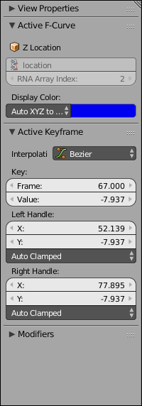
Figure 10-9: The Properties region (N) in the Graph Editor.
Often, you run into the occasion where you need to edit all the control points in a single frame so that you can change the overall timing of your animation. You may be tempted to use Border Select (B) to select the strip of control points you want to move around. However, a cleaner and easier way is to select one of the control points on the frame you want to adjust and press K in the Graph Editor or choose Select ⇒ Columns on Selected Keys. All the other control points that are on the same frame as your initial selection are selected.
Table 10-1 covers the most common hotkeys and mouse actions used to control animation in the Graph Editor.
Table 10-1 Commonly Used Hotkeys and Mouse Actions for the Graph Editor
|
Mouse Action |
Description |
Hotkey |
Description |
|
Left-click graph |
Move time cursor |
Alt+A |
Playback animation |
|
Left-click channel eye icon |
Hide/Reveal channel |
Shift+E |
Extrapolation Mode |
|
Left-click channel |
Select channel |
K |
Select columns of selected control points |
|
Right-click |
Select control point |
L |
Select linked control points |
|
Middle-click |
Pan graph |
O |
Clean keyframes |
|
Ctrl+middle-click |
Scale graph |
N |
Properties region |
|
Scroll |
Zoom graph |
Shift+S |
Snap Menu |
|
Shift+scroll |
Pan graph vertically |
T |
Interpolation Type |
|
Ctrl+scroll |
Pan graph horizontally |
Home |
Fit curves to graph |
Using F-curve modifiers
One of the biggest appeals of computer graphics in general — and computer animation specifically — is the prospect of letting the computer do all the hard work for you. Or at least you want the computer to handle a big chunk of the boring parts. If Blender's Graph Editor gives you the ability to procedurally manipulate f-curves with modifiers much in the same way that you can with meshes, that's something worth knowing about.
The preceding section addresses modifiers when covering the cyclic curve extrapolation mode (Shift+E). The Cycles modifier described there is one of a handful of f-curve modifiers that you can add. The following is a brief run-down of each of the f-curve modifier's that Blender offers:
· Generator: This modifier generates a new curve based on basic mathematical formulas for lines, parabolic lines, and some more advanced curve shapes. Unless you use additive mode, it completely disregards any existing keyframes on your f-curve.
· Built-In Function: This modifier generates a curve based on a different set of mathematical formulas than the Generator f-curve modifier. The formulas in this modifier are more naturally cyclic, like sine waves and tangent curves. Like the Generator f-curve modifier, this modifier also completely disregards any existing keyframes on your f-curve unless you use additive mode.
· Envelope: Though it can be a bit difficult to control, the Envelope f-curve modifier is extremely powerful. It's like the envelopes in audio processing software. You can add control points to define upper and lower thresholds for your f-curve. Any values in the f-curve beyond those thresholds (outside of the envelope) are attenuated (reduced so they fit within the envelope's bounds).
· Cycles: As covered previously in this chapter, this f-curve modifier duplicates your existing keyframes, repeating them over time.
· Noise: With the Noise f-curve modifier, you can add random variation to your f-curve.
Used judiciously, this modifier can bring a lot of life to an animation. For example, you could animate a car rolling along a bumpy road without actually creating those bumps at all.
· Python: With a little bit of programming knowledge, you can use Python to have nearly unlimited control over the behavior of an f-curve. Python coding, however, is an advanced topic and out of the scope of this book.
· Limits: This f-curve modifier is similar to the Envelope f-curve modifier, except you can't set arbitrary control points. You just have minimum and maximum X- and Y-axis control values for your f-curve. Also, rather than attenuating your f-curve when it exceeds those controls, the Limits f-curve modifier simply clips, or cuts off the overshoot segments of the f-curve.
· Stepped Interpolation: Using the Stepped Interpolation f-curve modifier, you can give your f-curve a stepped appearance as it goes from one keyframe to the next. It would be like using constant interpolation on your f-curve and inserting a keyframe on every frame of your animation. This can be useful if you want to give your animation a strobed or stop-motion look.
Figure 10-10 shows the panel for each of the f-curve modifiers.
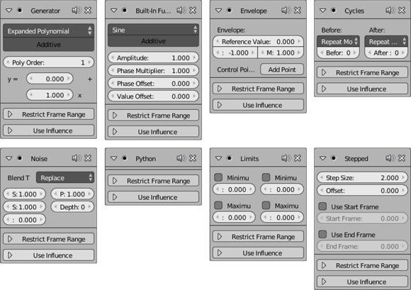
Figure 10-10: Blender offers eight different f-curve modifiers that you can apply to f-curves in your animation.
Like the modifiers that affect your 3D objects (see Chapter 5), you can stack f-curve modifiers so each one contributes to the one before it. For example, you could start with the Built-In Function f-curve modifier on your object's Z location to have your object move up and down sinusoidally. Then you could add a Noise f-curve modifier so it stutters a bit as it moves up and down.
Using Constraints Effectively
Occasionally, I get into conversations with people who assume that because there's a computer involved, good CG animation takes less time to make than traditional animation. In most cases, this assumption isn’t true. High-quality work takes roughly the same amount of time, regardless of the tool. The time is just spent in different places. Whereas in traditional animation, a very large portion of the time is spent drawing the in-between frames, CG animation lets the computer handle that detail. However, traditional animators don't have to worry as much about optimizing for render times, tweaking and re-tweaking simulated effects, or modeling, texturing, and rigging characters.
That said, computer animation does give you the opportunity to cut corners in places and make your life as an animator much simpler. Constraints are one feature that fit this description perfectly. Literally speaking, a constraint is a limitation put on one object by another, allowing the unconstrained object to control the behavior of the constrained one.
With constraints, you can do quite a lot without doing much at all. Animation is hard work; it's worth it to be lazy whenever you can.
To see the actual constraints that you have available, go to Constraint Properties and left-click the Add Constraint button. Alternatively, you can press Shift+Ctrl+C in the 3D View. Either way, you see a menu similar to the one in Figure 10-11.
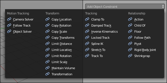
Figure 10-11: The types of constraints available by default within Blender.
In Chapter 4, I present a mnemonic for remembering how the parenting operation relates to the active object (children first!). For constraints, the mnemonic is a little bit backward because the active object is actually the object you're constraining. Because a constraint, by definition, restricts an object in some way, that object basically becomes a kind of prisoner. So for constraints, I think, “Prisoners last.” And there you have it, a handy mnemonic device for remembering selection order when parenting or constraining: children first (parenting) and prisoners last (constraining).
Because of limitations to this book's page count, I can't cover the function of each and every constraint in full detail. However, the remaining sections in this chapter cover features found in most constraints and some usage examples for more frequently used constraints.
The all-powerful Empty!
Of all the different types of objects available to you in Blender, none of them are as useful or versatile in animation as the humble Empty. An Empty isn't much — just a little set of axes that indicate a position, orientation, and size in 3D space. Empties don't even show up when you render. However, Empties are an ideal choice for use as control objects, and they're a phenomenal way to take advantage of constraints.
Empties can be displayed in the 3D View in a number of ways. Because an Empty can be used as a control for constraints and animations, sometimes it's useful to have it displayed with a particular shape. The following display types are available for Empties:
· Plain Axes: Think of this as the default display type. It's just a set of 3D crosshairs.
· Arrows: Occasionally, it's worthwhile to know specifically which axis is facing which direction on your Empty. This display type labels each axis in its positive direction.
· Single Arrow: This display type works great for a minimalist control. The arrow points along the Empty's local Z-axis.
· Circle: If you want an unobtrusive animation control, the Circle display type is a good choice. It allows your Empty to be located inside a volume (like an arm or leg), but still remain selectable because the circle is outside of it.
· Cube: Choose this display type and your Empty appears like a wireframe cube.
· Sphere: Like the Cube display type, this makes your Empty appear as a wireframe sphere.
· Cone: The Cube and Sphere display types can be handy, but they don't naturally give any indication of direction; you don't know which axis is up. The Cone display type draws your Empty like a wireframe cone with the point going along its local Z-axis.
· Image: With this display type, your Empty appears in the 3D View as a plane with any image you choose mapped to it. This display type isn't particularly useful as a controller for a constraint, but it's pretty useful in modeling. You can have a reference image visible in your 3D View from any direction.
As a practical example of how useful Empties can be, consider that 3D modelers like to have a turnaround render of the model they create. Basically, a turnaround render is like taking the model, placing it on a turntable, and spinning it in front of the camera. It's a great way to show off all sides of the model. Now, for simple models, you can just select the model, rotate it in the global Z-axis, and you're done. However, what if the model consists of many objects, or for some reason everything is at a strange angle that looks odd when spun around the Z-axis? Selecting and rotating all those little objects can get time consuming and annoying. A better way of setting up a turnaround is with the following rig:
1. Add an Empty (Shift+A⇒Empty⇒Plain Axes).
2. Grab the Empty to somewhere at the center of the model (G).
3. Select the camera and position it so that the model is in the center of view (right-click, G).
4. Add the Empty to your selection (Shift+right-click).
5. Make the Empty the camera's parent (Ctrl+P⇒Object).
6. Select the Empty and insert a rotation keyframe (right-click, I⇒Rotation).
7. Move forward in time 50 frames.
8. Rotate the Empty 90 degrees in the Z-axis and insert a new rotation keyframe (R⇒Z⇒90, I⇒Rotation).
The camera obediently matches the Empty's rotation.
9. Bring up the Graph Editor and set the extrapolation mode for the Z Rotation channel to linear extrapolation (Shift+F6, left-click, Shift+E⇒Linear Extrapolation).
10. Switch back to the 3D View and set it to use the camera view. Then playback the animation (Shift+F5, Numpad 0, Alt+A).
In the 3D View, you see your model spinning in front of your camera.
In this setup, the Empty behaves as the control for the camera. Imagine that a beam extends from the Empty's center to the camera's center and that rotating the Empty is the way to move that beam.
Adjusting the influence of a constraint
One of the most useful settings that's available to all constraints is at the bottom of each constraint block: the Influence slider. This slider works on a scale from 0 to 1, with 0 being the least amount of influence and 1 being the largest amount. With this slider, you have the capability of just partially being influenced by the target object's attributes. There's more to it, though.
You can animate any attribute in the Properties editor by right-clicking it and choosing Insert Keyframe (or pressing I with your mouse cursor hovered over that property), which means you can easily animate the influence of the constraint. If you key the Influence value of a constraint, a curve for that influence becomes visible in the Graph Editor.
Say that you're working on an animation that involves a character with telekinetic powers using his ability to make a ball fly to his hand. You can do that by animating the influence of a Copy Location constraint (see the “Copying the movement of another object” section) on the ball. The character's hand is the target, and you start with 0 influence. Then, when you want the ball to fly to his hand, you increase the influence to 1 and set a new keyframe. KERPLOW! Telekinetic character!
Using vertex groups in constraints
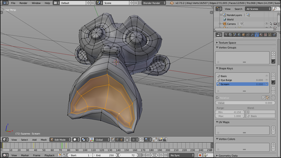
Many constraints have a Vertex Group field that appears after choosing a valid mesh object in the Target field. In the Vertex Group field, you can type or choose the name of a vertex group in the parent mesh. When you do, the constrained object is bound only to those specific vertices. (See Chapter 11 for details on how to create a vertex group.) After you choose a vertex group from the Vertex Group field of your constraint, the relationship line from the constrained object changes to point to the vertices in that group. Figure 10-12 shows a Suzanne head with a Child Of constraint bound to a vertex group consisting of a single vertex on a circle mesh.
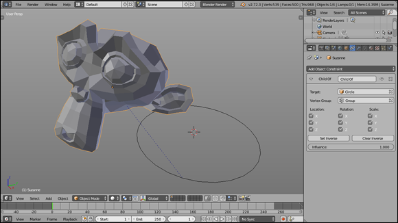
Figure 10-12: Parenting an object to a vertex group.
Copying the movement of another object
Using simple parenting is helpful in quite a few instances, but it's often not as flexible as you need it to be. You can't control or animate the parenting influence or use only the parent object's rotation without inheriting the location and scale as well. And you can't have movement of the parent object in the global X-axis influence the child's local X-axis location. More often than not, you need these sorts of refined controls rather than the somewhat ham-fisted Ctrl+P parenting approach.
To this end, a set of constraints provide you with just this sort of control: Copy Location, Copy Rotation, and Copy Scale. Figure 10-13 shows what each constraint looks like when added in Constraint Properties.
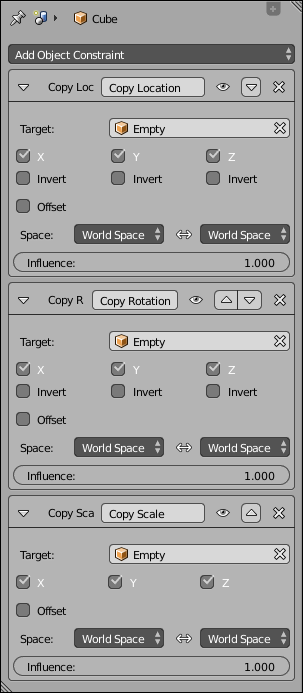
Figure 10-13: The Copy Location, Copy Rotation, and Copy Scale constraint controls.
You can mix and match multiple constraints on a single object in a way that's very similar to the way you can add multiple modifiers to an object. So if you need both a Copy Location and a Copy Rotation constraint, just add both. After you add them, you can change which order they come in the stack to make sure that they suit your needs.
Words and picture aren't always the best way of explaining how constraints work. It's often more to your benefit to see them in action. To that end, the website that accompanies this book has a few example files that illustrate how these constraints work. It's worth it to load them up in Blender and play with them to really get a good sense for how these very powerful tools work.
Probably the most apparent thing about these Copy constraints is how similar their options are to one another. The most critical setting, however, is the object that you choose in the Target field. If you're using an Empty as your control object, this is where you choose that Empty or type its name (as mentioned in other chapters, you can also hover your mouse over the Target field and press E to enable Blender's eyedropper feature to let you click on the target object). Until you do so, the Constraint Name field at the top of the constraint block remains bright red and the constraint simply won't work.
Below the Target field are a series of six check boxes. The X, Y, and Z check boxes are enabled by default, and beneath them are corresponding disabled check boxes, each labeled Invert. These six check boxes control which axis or axes the target object influences. If the axis check box is enabled and the Invert check box below it is also enabled, the target object has an inverted influence on the constrained object in that axis. Using the preceding Copy Location example, if you disable the X check box and then grab the Empty and move it in the X-axis (G⇒X), the cube remains perfectly still. However, enabling the X check box as well as the Invert check box beneath it causes the cube to translate in an opposite X direction when you move the target Empty.
Next up is the Offset check box, which is useful if you've already adjusted your object's location, rotation, or scale prior to adding the constraint. By default, this feature is off, so the constrained object replicates the target object's behavior completely and exactly. With it enabled, though, the object adds the target object's transformation to the constrained object's already set location, rotation, or scale values. The best way to see this is to create a Copy Location constraint with the following steps:
1. Start with the default scene (Ctrl+N).
2. Grab the default cube to a different location (G).
3. Add an Empty (Shift+A⇒Empty⇒Plain Axes).
4. Add the cube to your current selection and put a Copy Location constraint on it (Shift+right-click, Shift+Ctrl+C⇒Copy Location).
The cube automatically snaps directly to the Empty's location.
5. Left-click the Offset check box in the Copy Location constraint within Constraint Properties.
The cube goes back to its original position. Grab (G) the Empty and its location influences the cube's location from there.
Putting limits on an object
Often when you animate objects, it's helpful to prevent objects from being moved, rotated, or scaled beyond a certain extent. Say that you're animating a character trapped inside a glass dome. As an animator, it can be helpful if Blender forces you to keep that character within that space. Sure, you could just pay attention to where your character is and visually make sure that he doesn't accidentally go farther than he should be allowed, but why do the extra work if you can have Blender do it for you? Figure 10-14 shows the constraint options for most of the limiting constraints Blender offers you.

Figure 10-14: The options for the limiting constraints that Blender offers you.
Here are descriptions of what each constraint does:
· Limit Location/Rotation/Scale: Unlike most of the other constraints, these three don't have a target object to constrain them. Instead, they're limitations on what the object can do within its own space. For any of them, you can define minimum and maximum limits in the X, Y, and Z axes. You enable limits by left-clicking their corresponding check boxes and define those limits in the value fields below each one.
The For Transform check box that's in each of these constraints can be pretty helpful when animating. To better understand what it does, go to the Properties region in the 3D View (N). If you have limits and For Transform is not enabled, the values in the Properties region change even after you reach the limits defined by the constraint. However, if you enable For Transform, the values in the Properties region are clipped to the limitations you defined with the constraint.
· Limit Distance: This constraint is similar to the previous ones except it relates to the distance from the origin of a target object. The Clamp Region menu gives you three ways to use this distance:
· Inside: The constrained object can only move within the sphere of space defined by the Distance value.
· Outside: The constrained object can never enter the sphere of space defined by the Distance value.
· On Surface: The constrained object is always the same distance from the target object, no more and no less.
The On Surface name is a bit misleading. Your object isn't limited to the surface of the target object; it's limited to the surface of an imaginary sphere with a radius equal to the Distance value.
· Floor: Technically, the Floor constraint is listed as a Relationship constraint, but I tend to think of it more as a limiting constraint. It uses the origin of a target object to define a plane that the origin of the constrained object can't move beyond. So, technically, you can use this constraint to define more than a floor; you can also use it to define walls and a ceiling as well. Remember, though, that this constraint defines a plane. If your target object is an uneven surface, it doesn’t use that object's geometry to define the limit of the constrained object, just its origin. Despite this limitation, this constraint is actually quite useful, especially if you enable the Use Rotation check box. This option allows the constrained object to recognize the rotation of the target object so that you can have an inclined floor, if you like.
When animating while using constraints, particularly limiting constraints, it's in your best interest to insert keyframes using Visual Location and Visual Rotation, as opposed to plain Location and Rotation. Using the visual keying types sets the keyframe to where the object is located visually, within the limits of the constraint, rather than how you actually transformed the object. For example, assume that you have a Floor constraint on an object that you're animating to fall from some height and land on a floor plane that's even with the XY grid. For the landing, you grab (G) the object and move your mouse cursor 4 units below the XY grid. Of course, because of the constraint, your object stops following the mouse when it hits the floor. Now, if you insert a regular Location keyframe here, the Z-axis location of the object is set to -4.0 even though the object can't go below 0. However, if you insert a Visual Location key, the object's Z-axis location is set to what you see it as: 0. If you enable the For Transform check box on all of your constraints, you can get similar behavior and just use regular (non-visual) location and rotation keyframing.
Tracking the motion of another object
Tracking constraints are another set of helpful constraints for animation. Their basic purpose is to make the constrained object point either directly at or in the general direction of the target object. Tracking constraints are useful for controlling the eye movement of characters or building mechanical rigs like pistons. Figure 10-15 shows the options for three of Blender's tracking constraints.
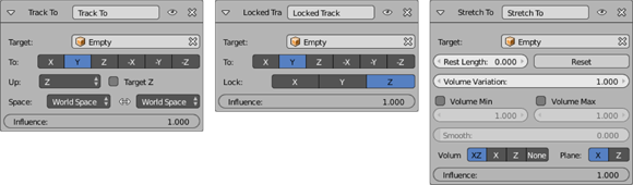
Figure 10-15: Control options for Blender's tracking constraints.
Following are descriptions of each tracking constraint:
· Track To: Of these constraints, this one is the most straightforward. In other programs, this constraint may be referred to as the Look At constraint, and that's what it does. It forces the constrained object to point at the target object. The best way to see how this constraint works is to go through the following steps:
· Load the default scene (Ctrl+N).
· Add a Track To constraint to the camera with the target object being the cube (right-click the cube, Shift+right-click the camera, Shift+Ctrl+C⇒Track To).
· In the buttons next to the To label, left-click -Z.
· In the Up drop-down menu, choose the Y-axis.
Now, no matter where you move the camera, it always points at the cube's origin. By left-clicking the X, Y, and Z buttons next to the To label and choosing an axes from the Up drop-down menu, you can control how the constrained object points relative to the target.
· Locked Track: The Locked Track constraint is similar to the Track To constraint, with one large exception: It only allows the constrained object to rotate on a single axis, so the constrained object points in the general direction of the target, but not necessarily directly at it. A good way to think about the Locked Track constraint is to imagine that you're wearing a neck brace. With the brace on, you can't look up or down; you can rotate your head only left and right. So if a bird flies overhead, you can't look up to see it pass. All you can do is turn around and hope to see the bird flying away.
· Stretch To: This constraint isn't exactly a tracking constraint like Track To and Locked Track, but its behavior is similar. The Stretch To constraint makes the constrained object point toward the target object like the Track To constraint. However, this constraint also changes the constrained object's scale relative to its distance to the target, stretching that object toward the target. And the Stretch To constraint can even preserve the volume of the constrained object to make it seem like it's really stretching. This constraint is great for cartoony effects, as well as for controlling organic deformations, such as rubber balls and the human tongue. On a complex character rig, you can use the Stretch To constraint to help simulate muscle bulging.
All materials on the site are licensed Creative Commons Attribution-Sharealike 3.0 Unported CC BY-SA 3.0 & GNU Free Documentation License (GFDL)
If you are the copyright holder of any material contained on our site and intend to remove it, please contact our site administrator for approval.
© 2016-2026 All site design rights belong to S.Y.A.