Essential MATLAB for Engineers and Scientists (2013)

PART 2

Applications

OUTLINE

Introduction

Chapter 12. Dynamical Systems

Chapter 13. Simulation

Chapter 14. Introduction to Numerical Methods

Chapter 15. Signal Processing

Chapter 16. SIMULINK

Chapter 17. Symbolics Toolbox

Introduction

Part 2 is on applications. Since this is an introductory course, the applications are not extensive. They are illustrative. You ought to recognize that the kinds of problems you actually can solve with MATLAB are much more challenging than the examples provided. However, many of the examples can be a starting point for the development of solutions to more challenging problems. The goal of this part of the text is to begin to scratch the surface of the true power of MATLAB.

CHAPTER 12

Dynamical Systems

Abstract

The objective of this chapter is to illustrate the importance of learning to use tools like MATLAB. MATLAB and companion toolboxes provide engineers, scientists, mathematicians, and students of these fields with an environment for technical computing applications. It is much more than a programming language like C or C++. Technical computing includes mathematical computation, analysis, visualization, and algorithm development. In this chapter we examine the application of MATLAB capabilities by solving four relatively simple problems in engineering science. The problems are the deflection of a cantilever beam subject to a uniform load, a single-loop closed electrical circuit, the free fall problem with friction, and the projectile problem with friction.

Keywords

Dynamical systems; Cantilever beam; Electrical circuit; Free-fall (with friction); Projectile (with friction)

CHAPTER OUTLINE

Cantilever beam

Electric current

Free fall

Projectile with friction

Summary

Exercises

The objective of this chapter is to discuss the importance of learning to use tools like MATLAB. MATLAB and companion toolboxes provide engineers, scientists, mathematicians, and students of these fields with an environment for technical computing applications. It is much more than a programming language like C, C++ or Fortran. Technical computing includes mathematical computation, analysis, visualization, and algorithm development. The MathWork website describes “The Power of Technical Computing with MATLAB” as follows:

■ Whatever the objective of your work—an algorithm, an analysis, a graph, a report, or a software simulation—technical computing with MATLAB lets you work more effectively and efficiently. The flexible MATLAB environment lets you perform advanced analyses, visualize data, and develop algorithms by applying the wealth of functionality available. With its more than 1000 mathematical, statistical, scientific and engineering functions, MATLAB gives you immediate access to high-performance numerical computing. This functionality is extended with interactive graphical capabilities for creating plots, images, surfaces, and volumetric representations.

■ The advanced toolbox algorithms enhance MATLAB's functionality in domains such as signal and image processing, data analysis and statistics, mathematical modeling, and control design. Toolboxes are collections of algorithms, written by experts in their fields, that provide application-specific numerical, analysis, and graphical capabilities. By relying on the work of these experts, you can compare and apply a number of techniques without writing code. As with MATLAB algorithms, you can customize and optimize toolbox functions for your project requirements.

In this chapter we are going to examine the application of MATLAB capabilities with four relatively simple problems in engineering science. The problems are the deflection of a cantilever beam subject to a uniform load, a single-loop closed electrical circuit, the free fall problem, and an extension of the projectile problem discussed in Chapter 2. The first problem is on a structural element you investigate in a first course in engineering mechanics. The structural element is the cantilever beam, which is one of the primary elements of engineered structures, e.g., buildings and bridges. We examine the deflection of this beam with a constant cross section when subject to a uniform distribution of load, e.g., its own weight.

The second problem is an examination of the equation that describes the “flow” of electrical current in a simple closed-loop electrical circuit. You examine this type of problem in a first course in electrical science.

The third problem is the free fall of an object in a gravitational field with constant acceleration, g. This is one of the first problems you examine in a first course in physics. We examine the effect of friction on the free-fall problem and, hence, learn that with friction (i.e., air resistance) the object can reach a terminal velocity.

The fourth problem is an extension of the projectile that takes into account air resistance (you learn about air resistance in your first course in fluid mechanics). By an examination of this problem, you will learn why golfers do not hit the ball from the tee at from the horizontal (which is the optimum angle for the furthest distance of travel of a projectile launched in frictionless air).

Before we begin, you must keep in mind that this is not a book on engineering or science; it is an introduction to the essential elements of MATLAB, a powerful technical analysis tool. In this and subsequent chapters you will scratch the surface of its power by solving some relatively simple problems that you have encountered or will encounter early in your science or engineering education. Keep in mind that MATLAB is a tool that can be used for a number of very productive purposes. One purpose is to learn how to write programs to investigate topics you confront in the classroom. You can extend your knowledge of MATLAB by self-learning to apply the utilities and any of the toolboxes that are available to you to solve technical problems. This tool requires a commitment from you to continue to discover and to use the power of the tool as part of your continuing education. Developing high-quality computer programs within the MATLAB environment in order to solve technical problems requires that you use the utilities available. If you need to write your own code you should, if at all possible, include the utilization of generic solvers of particular types of equations that are available in MATLAB. Of course, to do this you need to learn more advanced mathematics, science and engineering. You will certainly have the opportunity to do this after freshman year.

As a student majoring in science and engineering you will take at least five semesters of mathematics. The fifth course is usually titled Advanced Calculus, Advanced Engineering Mathematics, Applied Mathematics, or Methods of Mathematical Physics. Topics covered in this course are typically ordinary differential equations, systems of differential equations (including nonlinear systems), linear algebra (including matrix and vector algebra), vector calculus, Fourier analysis, Laplace transforms, partial differential equations, complex analysis, numerical methods, optimization, probability and statistics. By clicking the question mark (?) near the center of the upper-most tool bar in the MATLAB desk top, as you already know, opens the help browser. Scan the topics and find utilities and examples of approaches to solve problems in all of these subjects and more.

The Control Systems Toolbox is an example of one of the numerous engineering and scientific toolboxes that have been developed to advance the art of doing science and engineering. SIMULINK and Symbolics are also very important toolboxes. The latter two are included with your “student version” of MATLAB. One of the big advantages of SIMULINK, in addition to being a graphical algorithm-development and programming environment, is that it is useful when using the computer to measure, record and access data from laboratory experiments or data from industrial-process monitoring systems. Symbolics is very useful because it allows you to do symbolic mathematics, e.g., integrating functions like the ones you integrate in your study of the calculus. All of the mathematical subjects investigated by you, as a science or engineering major, are applied in your science and engineering courses. They are the same techniques that you will apply as a professional (directly or indirectly depending on the software tools available within the organization that you are employed). Thus, you can use your own copy of MATLAB to help you understand the mathematical and software tools that you are expected to apply in the classroom as well as on the job.

12.1. Cantilever beam

In this section we want to examine the problem of the cantilever beam. The beam and its deflection under load is illustrated in Figure 12.1 below, which is generated by the script m-file created to solve the problem posed next. Many structural mechanics formulas are available in Formulas for Stress and Strain, Fifth Edition by Raymond J. Roark and Warren C. Young, published by McGraw-Hill Book Company (1982). For a uniformly loaded span of a cantilever beam attached to a wall at with the free end at , the formula for the vertical displacement from under the loaded condition with y the coordinate in the direction opposite that of the load can be written as follows:

where , E is a material property known as the modulus of elasticity, I is a geometric property of the cross-section of the beam known as the moment of inertia, L is the length of the beam extending from the wall from which it is mounted, and w is the load per unit width of the beam (this is a two-dimensional analysis). The formula was put into dimensionless form to answer the following question: What is the shape of the deflection curve when the beam is in its loaded condition and how does it compare with its unloaded perfectly horizontal orientation? The answer will be provided graphically. This is easily solved by using the following script:

%

% The deflection of a cantilever beam under a uniform load

% Script by D.T.V. .............. September 2006, May 2016

%

% Step 1: Select the distribution of X's from 0 to 1

% where the deflections to be plotted are to be determined.

%

X = 0:.01:1;

%

% Step 2: Compute the deflections Y at eaxh X. Note that YE is

% the unloaded position of all points on the beam.

%

Y = - ( X.^4 - 4 * X.^3 + 6 * X.^2 );

YE = 0;

%

% Step 3: Plot the results to illustrate the shape of the

% deflected beam.

%

plot([0 1],[0 0],'--',X,Y,'LineWidth',2)

axis([0,1.5,-4, 1]),title('Deflection of a cantilever beam')

xlabel('X'),ylabel('Y')

legend('Unloaded cantilever beam','Uniformly loaded beam')

%

% Step 4: Stop

Again, the results are plotted in Figure 12.1. It looks like the beam is deflected tremendously. The actual deflection is not so dramatic once the actual material properties are substituted to determine y and x in, say, meters. The scaling, i.e., re-writing the equation in dimensionless form in terms of the unitless quantities Y and X, provides insight into the shape of the curve. In addition, the shape is independent of the material as long as it is a material with uniform properties and the geometry has a uniform cross sectional area, e.g., rectangular with height h and width b that are independent of the distance along the span (or length) L.

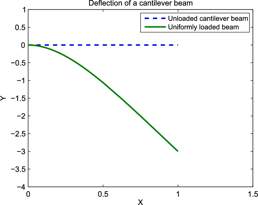
FIGURE 12.1 The vertical deflection of a uniformly loaded, cantilever beam.

12.2. Electric current

When you investigate electrical science you investigate circuits with a variety of components. In this section we will solve the governing equation to examine the dynamics of a single, closed loop electrical circuit. The loop contains a voltage source, V (e.g., a battery), a resistor, R (i.e., an energy dissipation device), an inductor, L (i.e., an energy storage device), and a switch which is instantaneously closed at time . From Kirchoff's law, as described in the book by Ralph J. Smith entitled Circuits, Devices, and Systems, published by John Wiley & Sons, Inc. (1967), the equation describing the response of this system from an initial state of zero current is as follows:

where i is the current. At the switch is engaged to close the circuit and initiate the current. At this instant of time the voltage is applied to the resistor and inductor (which are connected in series) instantaneously. The equation describes the value of i as a function of time after the switch is engaged. Hence, for the present purpose, we want to solve this equation to determine i versus t graphically. Rearranging this equation, we get

The solution, by inspection (another method that you learn when you take differential equations), is

This solution is checked with the following script:

%

% Script to check the solution to the soverning

% equation for a simple circuit, i.e., to check

% that

% i = (V/R) * (1 - exp(-R*t/L))

%

% is the solution to the following ODE

%

% di/dt + (R/L) * i - V/L = 0

%

% Step 1: We will use the Symbolics tools; hence,

% define the symbols as follows

%

syms i V R L t

%

% Step 2: Construct the solution for i

%

i = (V/R) * ( 1 - exp(-R*t/L) );

%

% Step 3: Find the derivative of i

%

didt = diff(i,t);

%

% Step 4: Sum the terms in ODE

%

didt + (R/L) * i - V/L;

%

% Step 5: Is the answer ZERO?

%

simple(ans)

%

% Step 6: What is i at t = 0?

%

subs(i,t,0)

%

% REMARK: Both answers are zero; hence,

% the solution is correct and the

% initial condition is correct.

%

% Step 7: To illustrate the behavior of the

% current, plot i vs. t for V/R = 1

% and R/L = 1. The curve illustrates

% the fact that the current approaches

% i = V/R exponentially.

%

V = 1; R = 1; L = 1;

t = 0 : 0.01 : 6;

i = (V/R) * ( 1 - exp(-R.*t/L) );

plot(t,i,'ro'), title(Circuit problem example)

xlabel('time, t'),ylabel('current, i')

%

When you run this script you will prove that the solution given above is correct. The figure that illustrates the solution to the problem posed is reproduced in Figure 12.2. This concludes this exercise related to electrical circuit theory that you will learn more about in your course on electrical science.

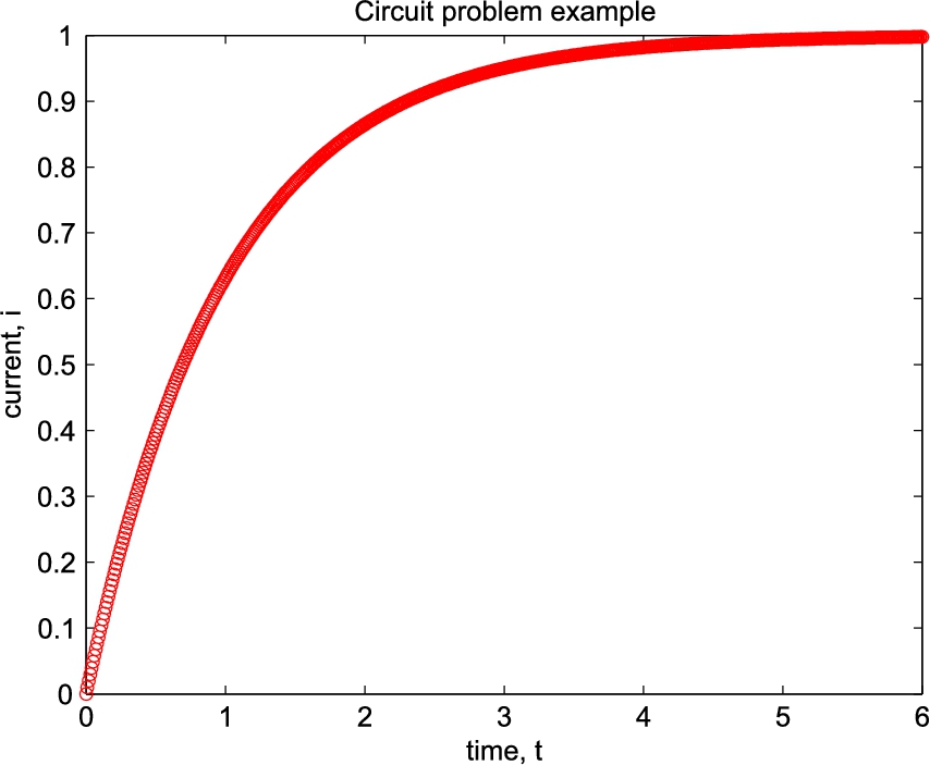
FIGURE 12.2 Exponential approach to steady current condition of a simple RL circuit with an instantaneously applied constant voltage.

12.3. Free fall

In this section we are going to use MATLAB to not only investigate the problem of free fall with friction (or air resistance), we are going to use MATLAB to check the theoretical results found in the literature. This example deals with the application of MATLAB for computing and graphically presenting information for analysis of the problem of free fall. This investigation is to examine the effect of air resistance on the distance of free fall in 5 s from a location , where the object is initially at rest (y is in the direction of gravity). Hence, we want to determine the distance, that an object falls from a state of rest with and without air resistance. In the book entitled Introduction to Theoretical Mechanics by R.A. Becker, that was published by McGraw-Hill Book Company (1954), the equations for free fall are given. The three cases of interest are as follows:

1. Without air resistance:

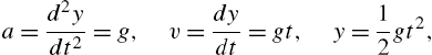
where a is the acceleration of the object, v is its speed and y is the distance of its free fall from the start of motion at .

2. With resistance proportional to the linear power of velocity:

3. With resistance proportional to the second power of velocity:

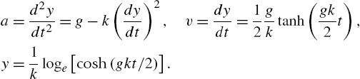
For all three cases the initial condition is at . (You will learn more about ordinary differential equations in your third semester of mathematics. In addition, in a first course in fluid mechanics you will learn about some of the details about air resistance. In particular, for air resistance associated with “laminar flow” problems, case 2 applies. In many practical situations it is case 3 that is usually the case of interest; this is the case where “turbulent flow” is important.)

Let us consider the following problem: Let us assume the above equations are correct. Note that they are written for a unit of mass. Let us also assume and for the air-drag parameter. Finally, let us answer the following:

(a) What is y in meters for s of free fall for the three cases.

(b) What are the terminal speeds in meters per second for cases 2 and 3 for the specified air-drag parameter?

(c) Is the terminal speed reached at s?

Note:

The terminal speeds are and for cases 2 and 3, respectively, where the terminal speed is the time independent or steady speed reached after a sufficient distance of free fall. It is the speed at which the gravitational force balances the air resistance force. From Part I, the Essentials, we learned that MATLAB is quite useful in this type of problem because it has the capability of computing the elementary functions in the formulas above.

As part of providing an answer to the questions raised, we want to examine the distance of free fall within the 5 s of flight time with the equations for y given above. Let us examine the influence of air resistance on free fall graphically; thus, we need to plot the distance y versus t from to . We shall plot all three curves on one figure for direct comparison. We will show that for a short period of time (significantly less than the 5 s) after the onset of motion all three curves are on top of each other. We will also show that at the distances of free fall are quite different.

The steps in the structure plan and the MATLAB code are as follows:

%

% Free fall analysis (saved as FFall.m):

% Comparison of exact solutions of free

% fall with zero, linear and quadratic

% friction for t = 0 to 5 seconds.

%

% Script by D. T. V. ......... September 2006.

% Revised by D.T.V. November 2008 & May 2016.

%

% Step 1: Specify constants

%

% Friction coefficient provided in the problem statement.

k = 0.2;

% Acceleration of gravity in m/s/s.

g = 9.81;

%

% Step 2: Selection of time steps for computing solutions

%

dt = .01;

%

% Step 3: Set initial condition (the same for all cases)

%

t(1) = 0.; v(1) = 0.; y(1) = 0.;

%

t = 0:dt:5;

%

% Step 4: Compute exact solutions at each time step

% from t = 0 to 5.

%

% (a) Without friction:

%

v = g * t;

y = g * t.^2 * 0.5;

%

% (b) Linear friction

%

velf = (g/k) * (1. - exp(-k*t));

yelf = (g/k) * t - (g/(k^2)) * (1.-exp(-k*t));

%

% (c) Quadratic friction

%

veqf = sqrt(g/k) * tanh( sqrt(g*k) * t);

yeqf = (1/k) * log(cosh( sqrt(g*k) * t) );

%

% Step 5: Computation of the terminal speeds

% (cases with friction)

%

velfT = g/k;

veqfT = sqrt(g/k);

%

% Step 6: Graphical comparison

%

plot(t,y,t,yelf,t,yeqf)

title('Fig 1. Comparison of results')

xlabel(' Time, t')

ylabel(' Distance, y ')

figure

plot(t,v,t,velf,t,veqf)

title('Fig. 2. Comparison of results')

xlabel(' Time, t')

ylabel(' Speed, v ')

%

% Step 7: Comparison of distance and speed at t = 5

%

disp(' ');

fprintf(' y(t) = %f, yelf(t) = %f, yeqf(t) = %f at t = %f\n',...

y(501),yelf(501),yeqf(501),t(501))

disp(' ');

fprintf(' v(t) = %f, velf(t) = %f, veqf(t) = %f at t = %f\n',...

y(501),yelf(501),yeqf(501),t(501))

%

% Step 8: Comparison of terminal velocity

%

disp(' ');

fprintf(' velfT = %f, veqfT = %f\n',...

velfT,veqfT)

%

% Step 9: Stop

%

The command window execution of the file above (named FFALL.m) gives the comparisons in Figures 12.3 and 12.4 and the printed results as follows:

>> FFall

y(t) = 122.625000, yelf(t) = 90.222433, yeqf(t) = 31.552121 at t = 5.000000

v(t) = 49.050000, velf(t) = 31.005513, veqf(t) = 7.003559 at t = 5.000000

velfT = 49.050000, veqfT = 7.003571

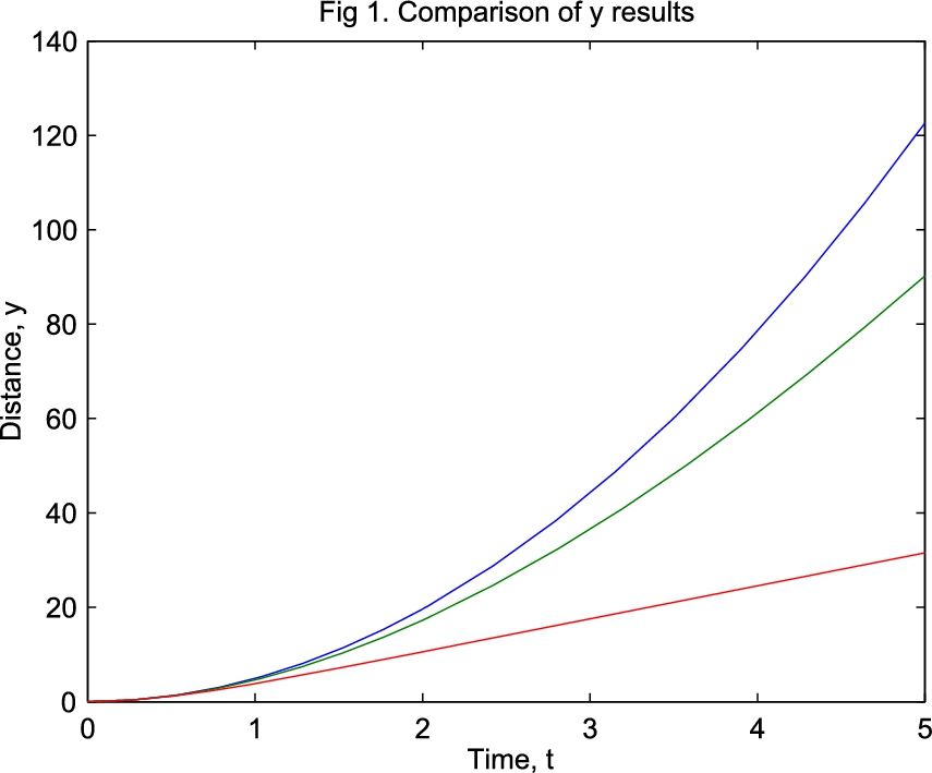
FIGURE 12.3 Comparison of free-fall distance: Top curve is for no friction, middle curve is for linear friction and the bottom curve is for quadratic friction.

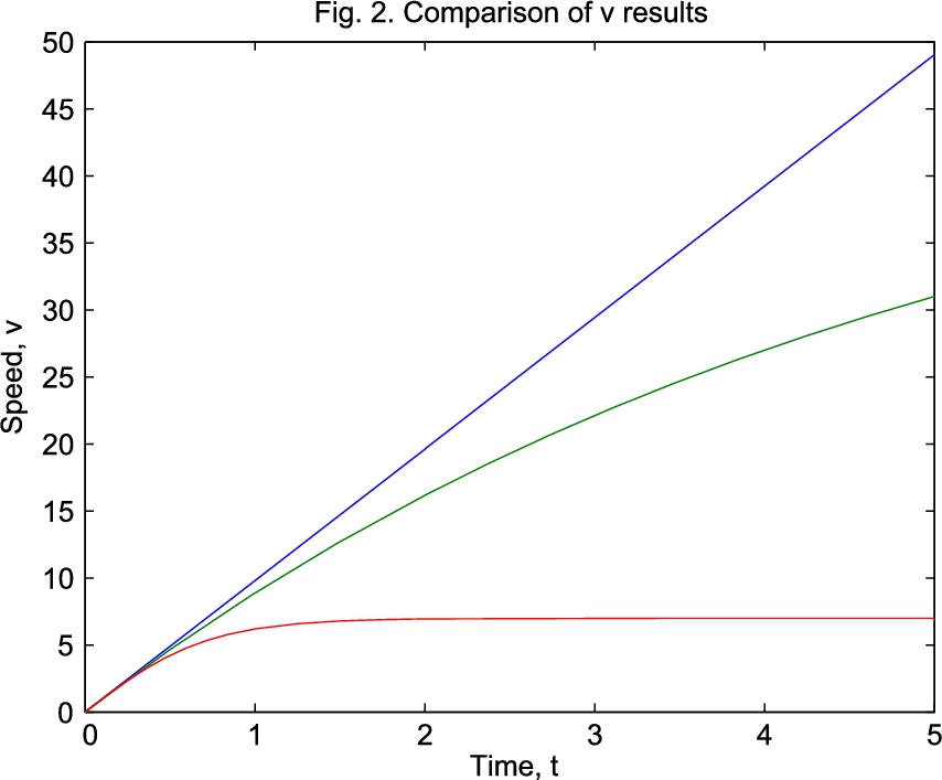
FIGURE 12.4 Comparison of free-fall speed: Top curve is for no friction, middle curve is for linear friction and the bottom curve is for quadratic friction.

The figures illustrate, as we may have expected, that for no friction the object falls the furthest distance. The case with quadratic friction reaches terminal velocity well within the five seconds examined. The linear friction case did not reach terminal speed, yet it is moving at a slower velocity as compared with the no friction case. Keep in mind that a unit mass object is falling with a friction coefficient . The same k was used for both the second and third cases. Within the first half second from the time of release the three curves are not distinguishable illustrating the fact that it takes a little time before the friction effects are felt. At the time of 5 s after release, the speed and the distance fallen are quite different. It is not surprising that quadratic friction slows the object quicker because the air resistance (or friction) is proportional to the speed squared, which is significantly larger than speed to the first power (as it is in the linear-friction case).

The above analysis was based on the exact solutions of the free-fall problem. Let use now use the symbolic tools to check the theoretical results found in the literature. The case that we will examine is Case 2, the linear friction case. The following script was implemented in the Command Window. The responses of MATLAB are also reproduced.

%

% The formula for the distance of free fall

% of an object from rest with linear friction

% is as follows:

%

% y = (g / k) * t - (g/k^2) * [ 1 - exp^(- k t)].

%

% To check the theory, we want to differentiate

% this twice to determine the formulas for velocity

% v and acceleration a, respectively. The results

% should match the published results.

%

% Step 1: Define the symblic variables

%

syms g k t y

%

% Step 2: Write the formula for y = f(t)

%

y = (g/k) * t - (g/k^2) * ( 1 - exp(-k * t));

%

% Step 3: Determine the velocity

%

v = diff(y,t);

%

% Step 4: Determine the acceleration

%

a = diff(v,t);

%

% Step 5: Print the v and a formulas and compare with

% the published results

%

v, a

%

% Step 6: Determine a from published formula and v.

%

a2 = g - k * v;

% Step 7: Simplify to somplest form

a2 = simple(a2)

%

% Step 6: Stop. REMARK: Results compare exactly. The

% results printed in the command window after executing

% this script are as follows:

% v = g/k-g/k*exp(-k*t)

% a = g*exp(-k*t)

% a2 = g/exp(k*t)

% These results verify the conclusion that the published

% formulas are correct.

%

Let us next consider an approximate method for solving the linear-friction case. This procedure is something you could have implemented if you didn't have the exact solution. More on numerical methods is provided in Chapter 14 of this book.

The equations for free-fall acceleration and velocity are differential equations. The following approximate analysis of a differential equation is called finite-differences. Let us consider the problem of free fall with linear friction (i.e., air drag that is linearly proportional to the speed of free fall). The formula (or equation) for this problem and its exact solution are given above. In the following analysis a script to solve this problem by the approximate method described below was written and executed for the same interval of time. This is described next. Then the approximate solution is compared with the exact solution graphically. For a unit mass, the formula that describes the velocity of free fall from rest with air resistance proportional to the linear power of velocity can be written as follows:

Let us approximate this equation by inverting the fundamental theorem of differential calculus, i.e., let us re-write it in terms of the definition of what a derivative is before the appropriate limit is taken. What is meant by this is to write this equation for a small interval of time as follows:

where the value identified by the integer n is the value of v at the beginning of the time interval, i.e., at . The value identified by is the value of v at the end of the time interval, i.e., at . This is an initial-value problem; hence, the value of v is known at . Knowing at , and by specifying , the value can be calculated by solving the finite-difference equation for given above. The solution will depend on the size of Δt. This formula gives us . We next need to solve for from the definition of v (viz., an approximate form of ). The average value of v over the interval of time, Δt, can be written in terms of y as follows:

Rearranging this equation, we get a formula for in terms of , , and Δt. Given the initial condition, i.e., and at , we compute with the first difference equation followed by computing with the last equation. Note that the new values become the initial condition for the next time step. This procedure is done repeatedly until the overall time duration of interest is reached (in this case this is ). The script file to implement this procedure is given next. The m-file is executed and the results plotted on the same graph with the exact solution. As shown, the comparison is remarkable. This is not always the case when approximate methods are used. The comparison is, of course, encouraging because we do not usually have exact results and need to resort to numerical approximations in our work.

The script file applied to examine the difference between the approximate method and the exact result is as follows:

%

% Approximate and exact solution comparison of

% free fall with linear friction for t = 0 to 5.

%

% Script by D. T. V. .......... September 2006.

% Revised by D.T.V. . November 2008 & May 2016.

%

% Step 1: Specified constants

%

k = 0.2;

g = 9.81;

%

% Step 2: Selection of time step for approximate solution

% dt = t(n+1) - t(n)

dt = 0.01;

%

% Step 3: Initial condition

%

t(1) = 0.;

v(1) = 0.;

y(1) = 0.;

%

% Step 3: Sequential implementation of the approximate

% solution method by repeating the procedure 500 times

% (using a for loop).

%

for n = 1:1:500

t(n+1) = t(n) + dt;

v(n+1) = (v(n) + dt * (g-0.5*k*v(n)) )/(1.+dt*0.5*k);

y(n+1) = y(n) + dt * 0.5 * (v(n+1) + v(n));

end

%

% Step 4: Exact solution over the same interval of time:

%

ye = (g/k) * t - (g/(k^2)) * (1.-exp(-k*t));

%

% Step 5: Graphical comparison:

%

plot(t,y,'o',t,ye)

title('Comparison of numerics w/ exact results')

xlabel(' Time, t')

ylabel(' Distance of free fall from rest, y')

%

% Step 6: Comparison of distance at t=5

%

disp(' ');

fprintf(' y(t) = %f, ye(t) = %f at t = %f \n',...

y(501),ye(501),t(501))

%

% Step 7: End of script by DTV.

%

In summary, the examination of the free fall problem illustrated the application and the checking of formulas reported in the literature. In addition, an approximate method was applied to solve the same problem to illustrate the application of a method that would be necessary if exact formulas were not found. Finally, the approximate method that was applied can certainly be improved by utilizing the ordinary differential equation solvers available in MATLAB. Examples of this type of procedure are given in Chapter 14. Other examples are in the help manuals in MATLAB that are found via the question mark (?) in the toolbar on the desktop window system (as already mentioned).

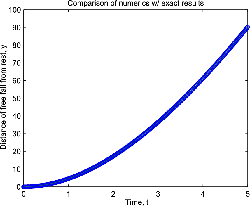
FIGURE 12.5 Comparison of free-fall distance. speed: Exact is the line, circles are for the finite-difference approximate solution.

12.4. Projectile with friction

Let is examine the projectile problem again. In this case let us examine the effect of air resistance on the flight of a projectile like a golf ball. For a unit mass, the formulas that describe the trajectory of a projectile in a gravitational field, g, with air resistance in the opposite direction of motion (that is proportional to the speed of the projectile in the direction of motion squared) are as follows:

The location of the projectile (e.g., a golf ball) is initially at , . It is launched at a speed in the direction of angle θ as measured from the horizontal. The coordinate x is in the horizontal direction parallel to the ground. The coordinate y is in the direction perpendicular to x pointing towards the sky. Hence, the gravitational acceleration is in the negative y direction. For a given launch speed and direction, we wish to estimate the range (or the distance) the ball travels in the x direction when it first hits the ground. To do this we shall approximate the four equations in a similar way that we treated the free falling object problem in the last section.

The solution method is given in detail in the script provided at the end of this paragraph. It was saved with the name golf.m.

%

% "The Golf ball problem"

% Numerical computation of the trajectory of a

% projectile launched at an angle theta with

% a specified launch speed. They are:

% theta = launch angle in degrees.

% Vs = launch speed.

%

% Script by D. T. V. ......... September 2006.

% Revised by D.T.V. November 2008 & May 2016.

%

% Equations of motion:

% u = dx/dt. v = dy/dt. g is in the opposite

% direction of y. x = y = 0 is the location of

% the tee. k is the coefficient of air drag. It

% is assumed to be constant. Friction is assumed

% to be proportional to the speed of the ball

% squared and it acts in the opposite direction

% of the direction of motion of the ball. The

% components of acceleration are thus:

% du/dt = - [k (u^2 + v^2) * u/sqrt(u^2+v^2)].

% dv/dt = - [k (u^2 + v^2) * v/sqrt(u^2+v^2)] - g.

%

% INPUT DATA

% Specified constants:

k = 0.02;

g = 9.81;

dt = 0.01;

%

% Input the initial condition:

%

theta = input(' Initial angle of launch: ')

the = theta * pi/180.;

Vs = input(' Initial speed of launch: ')

u(1) = Vs * cos(the);

v(1) = Vs * sin(the);

% Launch pad location:

x(1) = 0.;

y(1) = 0.;

%

% Compute approximate solution of the trajectory

% of flight.

% Repeat up to 6000 time, i.e., until ball hits

% the ground.

%

for n=1:1:6000;

u(n+1) = u(n) ...

- dt * (k * sqrt(u(n)^2+v(n)^2) * u(n));

v(n+1) = v(n) ...

- dt * (k * sqrt(u(n)^2+v(n)^2) * v(n) + g);

x(n+1) = x(n) + u(n) * dt;

y(n+1) = y(n) + v(n) * dt;

% Determination of when the object hits ground:

if y(n+1) < 0

slope = (y(n+1) - y(n))/(x(n+1) - x(n));

b = y(n) - slope * x(n);

xhit = - b/slope;

plot(x,y)

fprintf(' The length of the shot = %5.2f \n', xhit)

end

% Once object hits terminate the computations with a break:

if y(n+1) < 0; break; end

end

%

% Graphical presentation of the results:

%

if y(n+1) > 0

plot(x,y)

end

% ------ End of golf-ball script by DTV

What is the optimum launch angle for ? The answer to this question is described next for the launch speed of 100. Note that the optimum angle is the angle which gives the longest distance of travel (or greatest range). To compute the optimum angle the following script was executed after the lines with the input statements in the golf.m script were commented out by typing % at the beginning of the two lines with the input commands. The two lines in question were commented out as follows:

%

% In golf.m the following alterations were made

% prior to running this script!!!!!!

%

% % theta = input(' Initial angle of launch: ')

% % Vs = input(' Initial speed of launch: ')

%

% This script then finds the optimum angle for k = 0.2

% to compare with the zero friction case, which we know

% has the optimum launch angle of 45 degrees.

%

% Script by D. T. V. .......... September 2006.

% Revised by D.T.V. November 2008 & May 2016.

%

% Consider launch angles from 1 to 45 degrees

%

th = 1:1:45;

vs = 100; % Specified launch speed.

%

% Execute the modified golf.m file 45 times and save

% results for each executoion of golf.m

%

for i=1:45

theta = th(i)

golf % Execution of modified golf.m script.

xh(i) = xhit

thxh(i) = theta

end

% Find the maximum distance and the correponding index

[xmh,n] = max(xh)

% Determine the angle that the maximum distance occured.

opt_angle = thxh(n)

$ Display the results

disp(' optimum angle ')

disp( opt_angle )

% REMARK: For this case the result is 30 degrees.

% End of script

The optimum angle of launch for the case of nonlinear friction was computed and found to be equal to . Without friction it is . Hence, it is not surprising that golfers launch their best drives at angles significantly less than .

Summary

In this chapter we examined three problems using some of the utilities in MATLAB. We did the following:

■ We determined the shape of the deflection of a cantilever beam based on a published formula in the engineering literature. Thus, we could use the capability of MATLAB to do arithmetic with polynomials.

■ We examined the effect of friction on the free fall problem. In addition to computing the distance and speed of free fall based on published formulas, we checked the formulas with the symbolics tools and we also solved the problem by an approximate method to illustrate the range of possibilities at your disposal to solve technical problems.

■ We examined the projectile problem subjected to air resistance. We did this by applying the same type of approximate method as we applied in the free fall problem. We found that the optimum angle of launch with friction taken into account is less than (the frictionless value).

Exercises

12.1 Reproduce the script for the exact solutions for the free fall problem (called FFall.m) and execute it for a range of friction coefficients, e.g., and 0.3.

12.2 Use the symbolics tools in the same way they were used to check the formulas for the linear-friction case of free fall, to check the other two cases.

12.3 Reproduce the golf.m (projectile script) and look at the effect of varying the friction coefficient k. Look at and 0.03. What influence does friction have on the optimum angle for a launch speed of 100?