Essential MATLAB for Engineers and Scientists (2013)

PART 2 Applications

CHAPTER 17 Symbolics Toolbox

Abstract

With the Symbolics toolbox included in the MATLAB/SIMULINK suite of tools, this system of tools can be considered the mathematical handbook for scientists and engineers of the 21st century. The objective of this chapter is to introduce the Symbolic tools available within MATLAB. It is a useful set of tools for the application of mathematics in science and engineering. Examples of the application of the Symbolic capabilities have already been given elsewhere in this book to check analytic solutions found in the literature. In addition, predictions based on the analytic solutions were compared with predictions based on computational methods. The symbolic mathematical tools covered in this chapter are:

• Algebra: Polynomials, vectors and matrices.

• Calculus: Differentiation and integration.

• Transforms: Laplace and Z transforms.

• Generalized functions: Heaviside and Dirac.

• Systems of ordinary differential equations.

• The funtool, mupad and help.

Keywords

MuPAD; Computer algebra and calculus; Symbolic solutions

The objective of this chapter is to introduce the Symbolic tools available within MATLAB. It is a useful set of tools for the application of mathematics in science and engineering. Examples of the application of the Symbolic capabilities have already been given elsewhere in this book to check analytic solutions found in the literature. In addition, predictions based on the analytic solutions were compared with predictions based on computational methods. The symbolic mathematical tools covered in this chapter are:

■ Algebra: Polynomials, vectors and matrices.

■ Calculus: Differentiation and integration.

■ Transforms: Laplace and Z transforms.

■ Generalized functions: Heaviside and Dirac.

■ Systems of ordinary differential equations.

■ The funtool, MuPAD and help.

With the Symbolics toolbox MATLAB can be considered the “mathematical handbook” for the students of the 21st century. In the old days science and engineering students were required to purchase a “standard” mathematics handbook. Today, there are very few students, if any, who own and use a mathematics handbook. The computer and tools like MATLAB have changed this situation in a positive way. However, as for the second author of this book, it has been an interesting exercise to demonstrate that MATLAB is this century's handbook. In this chapter an introduction to the application of Symbolics follows a procedure based on a review of handbook information and providing examples for the kinds of information we were expected to look up in a handbook and, hence, what we, sort of, expect students to find by applying computer tools like MATLAB.

The main problem, if it is a problem at all, in the application of the symbolic toolbox, or any other computer tool that allows the user to do symbolic analysis, is that to use the tool effectively you need to know something about the mathematical questions being raised. In other words, if you want to differentiate the function, , with respect to the variable x, you need to know the meaning of a function and the meaning of differentiation or finding the derivative of f with respect to x, viz., finding .

Another example is finding the solutions of a quadratic equation. You need to know what kind of equation this is and the meaning of solving an algebraic equation of this type. Hence, if you know what to ask, MATLAB Symbolics can be applied to help you find an answer to a symbolic mathematical question.

The application of symbolics to examine mathematical questions that can be answered with the help of mathematical handbooks is addressed in this chapter to illustrate the power of the symbolic tools available in MATLAB. Certainly the tools are more powerful than the relatively simple examples presented in this chapter. Once you are adept at using this toolbox, then you can extend the application of this toolbox to examine more difficult questions that may even be beyond the capabilities of more traditional applications of applied mathematics to solve problems in science and in engineering.

The symbolic mathematical topics covered in a typical handbook are, e.g., algebra, trigonometry, calculus, integration, differentiation and differential equations. The information provided in a handbook is to help the student, engineer or scientist make progress in solving mathematical problems they confront in their attempts to solve technical problems. A solid education in science, technology, engineering and mathematics (STEM) provides the necessary background to utilize handbooks and/or tools like MATLAB in a productive way. Of course, MATLAB like handbooks need to be used regularly to gain proficiency in applying such tools as part of finding solutions. We will touch some of the topics covered in handbooks to help guide the readers in their attempts to apply the Symbolic toolbox within MATLAB. We will start with algebra including linear algebra, vector algebra and matrix algebra. Then we will examine differentiation and integration. This will be followed by investigating integral transforms and, in particular, the Laplace transform. Then we will conclude by investigating the symbolic solution of differential equations.

17.1. Algebra

In Section 1.1.6 we introduced how to solve a system of linear equations. One example applied the solve utility available in MATLAB Symbolics. Let us extend that example by solving the simultaneous system of quadratic equations

Applying the same procedure illustrated in Section 1.1.6, we get the following results by typing and executing the following command in the Command Window. The results are also illustrated below.

>> [x y] = solve('x^2 + 3*y', 'y^2 + 2*x')

x =

-(-12)^(2/3)/2

-((3^(1/2)*(-12)^(1/3)*i)/2 + (-12)^(1/3)/2)^2/2

-((3^(1/2)*(-12)^(1/3)*i)/2 - (-12)^(1/3)/2)^2/2

y =

(-12)^(1/3)

- (3^(1/2)*(-12)^(1/3)*i)/2 - (-12)^(1/3)/2

(3^(1/2)*(-12)^(1/3)*i)/2 - (-12)^(1/3)/2

The results indicate that x and y each have four roots. Two are real and two are complex. This points to the fact that MATLAB deals with complex numbers and, hence, not just real numbers. This is another important capability of MATLAB. In MATLAB by default (unless you reassign them) i and j represent the number known as .

17.1.1. Polynomials

Everyone reading this book certainly knows about the quadratic equation. Most students of STEM subjects can recite, from memory, the roots of the quadratic equation; this is helpful to check the results found by applying MATLAB. The quadratic equation can be written as follows:

(17.1)

Let us solve this equation using the solve utility in MATLAB. To do this we can execute the following script:

clear;clc

syms a b c x

solve(a*x^2 + b*x + c)

The answer in the Command Window is

ans =

-(b + (b^2 - 4*a*c)^(1/2))/(2*a)

-(b - (b^2 - 4*a*c)^(1/2))/(2*a)

Thus, as expected, the solutions of the quadratic equation are

(17.2)

For the two roots to be real numbers . If the equality holds, then the two roots are equal. If the roots are complex and unequal. An alternative one-line command can be used to solve this equation; this can be done in the Command Window as follows

>> solve('a*x^2+b*x+c')

The apostrophes indicate that what is between them is a symbolic expression. The output of both procedures of the application of solve is a symbolic data-type array. Since this is a quadratic equation we expect to get two solutions.

Next, let us examine the cubic polynomial

(17.3)

To find the roots of this equation we can execute the following script:

clear;clc

syms a b c d x

solve(a*x^3 + b*x^2 + c*x + d)

In this case, since we are solving a cubic, the answer (ans) is in a symbolic data-type array. The answer is rather lengthy however and, hence, it is not reproduced here. It is produced in the command window.

Let us consider another example. Let us solve

The following commands were executed in the Command Window:

>> solve('a*x^4 + c*x ');

>> solution = simple(ans);

>> solution

solution =

(-c/a)^(1/3)

((3^(1/2)*i - 1)*(-c/a)^(1/3))/2

-((3^(1/2)*i + 1)*(-c/a)^(1/3))/2

>> latex(solution)

ans =

\left(\begin{array}{c} 0\\ {\left(-\frac{c}{a}\right)}^{\frac{1}{3}}\\

\frac{\left( - 1 + \sqrt{3}\, \mathrm{i}\right)\,

{\left(-\frac{c}{a}\right)}^{\frac{1}{3}}}{2}\\

-\frac{\left(1 + \sqrt{3}\, \mathrm{i}\right)\,

{\left(-\frac{c}{a}\right)}^{\frac{1}{3}}}{2} \end{array}\right)

This answer (ans) was used in the word processor used by the second author; the word processor implements Latex. This translation to Latex gives the following array of the four roots to this quartic equation:

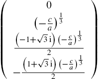
Note that two of the roots are complex numbers.

Finally, let us examine the solution of three simultaneous linear equations with the solve utility. Let us solve

Doing this in the Command Window, we get

>> [x y z] = solve('x + y + z = 1','2*x + 3*y + z = 1',

'x + y + 3*z = 0')

The solution of this system of equations leads to , and .

Note that there are a variety of methods to implement the solve function (or solution procedure utility) within Symbolics. If numerical solutions are obtained, as in the last example, they need to be converted to double data types to use them in MATLAB scripts (this was already illustrated in Section 1.1.6).

17.1.2. Vectors

The single row or single column arrays are vectors. Let us consider the following 3-component vectors:

There are two ways to multiply these mathematical objects that most of the students are familiar. They are the inner or dot product and the vector or cross product. They can be found by applying the following script of Symbolic commands (from the editor).

format compact

syms a1 a2 b1 b2 c1 c2 real

x1 = [a1,b1,c1]

x2 = [a2,b2,c2]

x1_dot_x2 = dot(x1,x2)

x1_cross_x2 = cross(x1,x2)

format

The results in the Command Window are

x1 =

[ a1, b1, c1]

x2 =

[ a2, b2, c2]

x1_dot_x2 =

a1*a2 + b1*b2 + c1*c2

x1_cross_x2 =

[ b1*c2 - b2*c1, a2*c1 - a1*c2, a1*b2 - a2*b1]

The format compact was implemented to get the compact output illustrated above. The last command, viz., format, was implemented to reset the default output-display format in the Command Window. The solution can be written as follows:

The dot product is a scalar.

The cross product is a vector. It is a three-component vector (the same number of components as the vectors that are multiplied to get this result).

17.1.3. Matrices

Let us consider the following mathematical objects known as matrices. We can add and subtract the two objects. We can multiply and divide the two objects. We will do these operations using the Symbolic toolbox

The following script was executed in MATLAB:

format compact

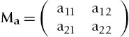
syms a11 a12 a21 a22 b11 b12 b21 b22

Ma = [a11 a12; a21 a22]

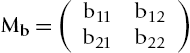
Mb = [b11 b12; b21 b22]

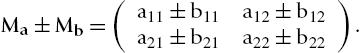
Msum = Ma + Mb

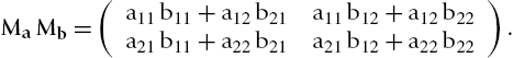
Mproduct = Ma*Mb

The results in the Command Window are

Ma =

[ a11, a12]

[ a21, a22]

Mb =

[ b11, b12]

[ b21, b22]

Msum =

[ a11 + b11, a12 + b12]

[ a21 + b21, a22 + b22]

Mproduct =

[ a11*b11 + a12*b21, a11*b12 + a12*b22]

[ a21*b11 + a22*b21, a21*b12 + a22*b22]

The addition of the two matrices involve term-by-term addition.

The product leads to a matrix of the same size as the matrices that are multiplied; each term in the result is the multiplication of the a row of times the column on summed together. Study the product matrix, as written below, to verify the matrix multiplication process. The product of the two matrices is

Let us analyze a number of properties of the following matrix:

syms c11 c12 c21 c22 real

Mc = [c11 c12; c21 c22]

Mcdet = det(Mc);

Mcinv = inv(Mc);

Mc*inv(Mc);

disp(' Mc * Mcinv = Imatrix')

Imatrix = simple(ans)

Mcdet

Mcinv

[EigenVectorsMc EigenValuesMc] = eig(Mc)

Except for the eigenvectors and eigenvalues, the following output was in the Command Window. The latter were converted to Latex and are reported below.

Mc =

[ c11, c12]

[ c21, c22]

Mc * Mcinv = Imatrix

Imatrix =

[ 1, 0]

[ 0, 1]

Mcdet =

c11*c22 - c12*c21

Mcinv =

[ c22/(c11*c22 - c12*c21), -c12/(c11*c22 - c12*c21)]

[ -c21/(c11*c22 - c12*c21), c11/(c11*c22 - c12*c21)]

The eigenvalues associated with this matrix are

This is a result of diagonalizing the matrix (a process interpreted geometrically as a rotation of the coordinate system to find the coordinates in which the matrix only has finite diagonal terms). The coordinate system at which this occurs is given by the orthogonal eigenvectors. The corresponding eigenvectors for this example are

Let us next consider the analysis of a three-by-three symmetric matrix, viz.,

This matrix was examined in detail by implementing the following script. It is an important mathematical object that plays an important role in, e.g., structural mechanics where it is the form of the stress tensor.

format compact

syms a b c d e f real

M = [a d e

d b f

e f c]

Mdet = det(M);

Minv = inv(M);

M*inv(M);

disp(' M * Minv = Imatrix')

Imatrix = simple(ans)

Mdet

Minv

[EigenVectorsM EigenValuesM] = eig(M)

format

The results in the Command Window, except for the rather lengthy eigenvalue, eigenvector and inverse expressions are as follows:

M =

[ a, d, e]

[ d, b, f]

[ e, f, c]

M * Minv = Imatrix

Imatrix =

[ 1, 0, 0]

[ 0, 1, 0]

[ 0, 0, 1]

Mdet =

- c*d^2 + 2*d*e*f - b*e^2 - a*f^2 + a*b*c

We know that the inverse of M is determined correctly because , where I is the identity matrix. It is left as an exercise to examine the inverse matrix and the results of the eigenvalue problem solved by the Symbolic tools in MATLAB.

If the matrix represents the state of stress at a point in a solid material, the eigenvalues would be the principal stresses and the eigenvectors the principal directions. This information is important in the analysis of the strength of materials. Similar matrices appear in modeling the mechanics of fluids.

17.2. Calculus

In this section we examine symbolic differentiation and integration. We will do this simultaneously because they are essentially inverse operation. Let us examine the quadratic function

(17.4)

The derivative of this equation is

(17.5)

This can be verified by applying the Symbolic tools in MATLAB. We can do this as follows:

format compact

syms x a b c real

f = a*x^2 + b*x + c

disp('dfdx = diff(f,x) was executed to get:')

dfdx = diff(f,x)

% Integration

disp('f = int(dfdx,x) was executed to get:')

f = int(dfdx,x)

disp(' Note that the constant of integration, c, is implied.')

disp(' Hence, to include it you need to add c to f:')

f = f + c

disp('f = expand(f) was executed to get:')

f = expand(f)

disp(' Thus, the function f is recovered (as expected).')

format

The output to the Command Window is

f =

a*x^2 + b*x + c

dfdx = diff(f,x) was executed to get:

dfdx =

b + 2*a*x

f = int(dfdx,x) was executed to get:

f =

x*(b + a*x)

Note that the constant of integration, c, is implied.

Hence, to include it you need to add c to f:

f =

c + x*(b + a*x)

f = expand(f) was executed to get:

f =

a*x^2 + b*x + c

Thus, the function f is recovered (as expected).

Thus, we verified the formula for . The next step is to verify the results of differentiation by integrating. This was done in the script given above by executing int(dfdx,x). The result obtained is f to within a constant. The integration tool does not explicitly include the arbitrary constant of integration. Hence, a constant needs to be added as illustrated in the above example. Then the function f with the added constant is expanded (expand(f)), leading to the result sought, i.e., the recovery of the original function f.

Let us examine a second example. It is the examination of

(17.6)

Differentiating this formula and, subsequently, integrating , we get the following: The script in the editor that was executed is

format compact

syms x a b c real

f = a*sin(x)^2 + b*cos(x)

dfdx = diff(f,x)

% Integration

ff = int(dfdx,x)

ff = expand(ff)

format

The output to the Command Window is

f =

a*sin(x)^2 + b*cos(x)

dfdx =

2*a*cos(x)*sin(x) - b*sin(x)

ff =

2*(cos(x)/2 + 1/2)*(2*a + b - 2*a*(cos(x)/2 + 1/2))

ff =

a + b + b*cos(x) - a*cos(x)^2

Note that the result of the integration of is (it is ff in the script; it is f below)

Substituting , we get

where c is the arbitrary constant of integration. Since it is arbitrary, let us select it as . Thus,

This is the result sought; it is the same as given in the original equation, Equation (17.6). Thus, these tools not only allow you to do differentiation and integration of a variety of problems you may confront in practice or wish to examine as part of your self-education, it helps provide insight into the connection between the operation of differentiation and the inverse operation of integration. We needed to be aware of the arbitrary constant of integration and what role it plays in the recovery of the formula that was differentiated. We needed to know that the derivative of a constant is identically zero.

17.3. Laplace and Z transforms

In this section the useful transforms known as the Laplace and the Z transforms are introduced by way of an example. Transforms are useful in applied mathematics as applied to examine engineering and scientific problems. There are other transforms available in Symbolics that could be investigated as well. We limit this primarily to the Laplace transform because it is introduced to undergraduates as part of the mathematics background necessary to examine dynamical systems. We examine the Z transform because it is interesting. In addition, we demonstrate the application of ezplot that is available in the Symbolic tools to help examine graphically various functions.

Let us examine the Laplace and the Z transforms of the function . Execute the following set of commands either in the Command Window or from the editor.

syms x t w

y = sin(x)

Ly = laplace(y)

yy = ilaplace(Ly,x)

Zy = ztrans(y)

ezplot(Ly)

hold on

ezplot(Zy)

ezplot(y)

The script in sequence determines the Laplace transform of y, Ly, it finds the inverse Laplace transform of the result to illustrate that you recover y, it determines the Z transform, Zy, (whatever that is) and it plots y, Ly and Zy. The results, as given in the Command Window, are as follows:

y =

sin(x)

Ly =

1/(s^2 + 1)

yy =

sin(x)

Zy =

(z*sin(1))/(z^2 - 2*cos(1)*z + 1)

The graphical results are in Figure 17.1.

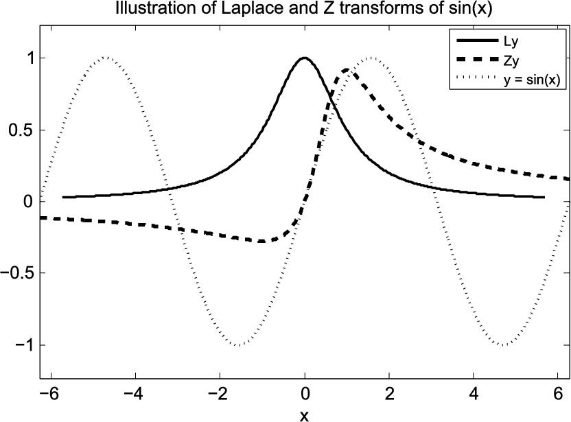
FIGURE 17.1 Comparison if sin x, its Laplace and Z transforms.

17.4. Generalized functions

In this section we examine very useful functions that are utilized in many scientific and engineering analyses. The first of the two functions examine is the Heaviside step function, . It is a function that is zero for , it is equal to 1/2 at and it is equal to unity for . It is a built in function in MATLAB and in MATLAB Symbolics. To examine it the following script was executed.

syms x

y = heaviside(x)

dydx = diff(y,x)

x = -1:.01:1;

y = heaviside(x);

plot(x,y,'--o'),title('The Heaviside step function')

xlabel('x');ylabel('y');

The output to the Command Window is

y =

heaviside(x)

dydx =

dirac(x)

Thus, the derivative of the Heaviside step function is the Dirac delta function (which we will examine next). A graphical illustration of the Heaviside step function is given in Figure 17.2.

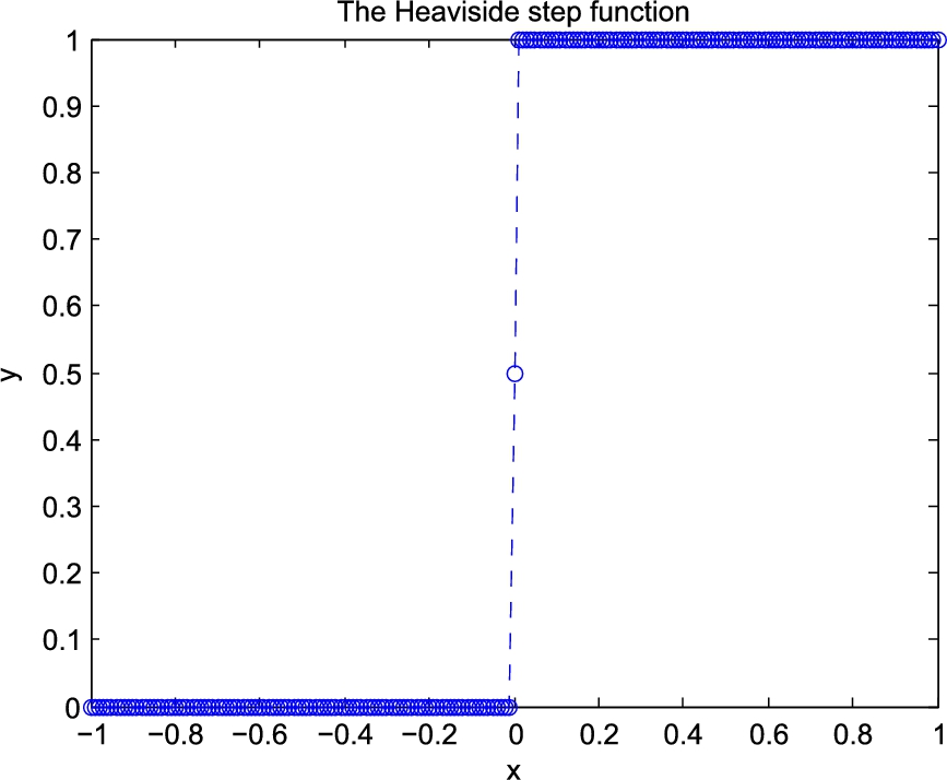
FIGURE 17.2 The Heaviside step function, H(x).

To use the Symbolic tools to examine the Dirac delta function let us execute the following script:

syms x

y = dirac(x)

I1 = int(y,x)

I2 = int(y,x,-1,1)

The results in the Command Window are as follows:

y =

dirac(x)

I1 =

heaviside(x)

I2 =

This illustrates that the indefinite integral of the Dirac function is the Heaviside function. It also illustrates that the definite integral that includes is one. The Dirac function is infinite at and it is zero everywhere else. It is not included in the range of integration the integral is zero. Note that where the delta function is infinite and, hence, where the Heaviside step function jumps from zero to one can be changed by changing the x coordinate to another origin where the argument of the two functions is equal to zero.

17.5. Differential equations

The function dsolve is an ordinary differential equation and a system of ordinary differential equation (ODE) solver. We will examine two examples in this section. One is the solution of a single ODE and a system of ODEs. Let us examine the equation

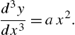
To solve this equation all we need to do is to execute the following command:

>> dsolve('D3y= a*x^2','x')

The result of executing this command is

ans =

(a*x^5)/60 + (C2*x^2)/2 + C3*x + C4

Thus, the solution is

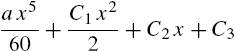
where , and are the three arbitrary constants of integration. The procedure for solving a differential equation is to integrate. In this case because it is a third-order differential equation that we solved, it required three integrations and, hence, the result is to within three arbitrary constants.

In the next example we solve two equations simultaneously. In addition, we specify constraints (or boundary conditions). The equations to be solved are

This system of equations, since it is second order, is subject to two constraints. In this example they are and , which can be interpreted as initial conditions. The solution can be obtained by implementing the following command in MATLAB:

[f, g] = dsolve('Df = 3*f + 4*g, Dg = -4*f + 3*g','f(0) = 0,

g(0) = 1')

The solution is

f =

sin(4*t)*exp(3*t)

g =

cos(4*t)*exp(3*t)

Thus,

The dsolve function is a powerful function to apply to try to find analytic solutions to systems of ODEs.

17.6. Implementation of funtool, MuPAD and help

This is the last section of this chapter. In this section we illustrate funtool, an interesting utility to examine graphically a variety of functions. The MuPAD capability to create your own notebooks associated with your own investigations is introduced. Finally, the help documents that come with MATLAB that are related to Symbolics is reviewed.

17.6.1. The funtool

In the Command Window type funtool and execute the command. This is done as follows:

>> funtool

The three windows illustrated in Figure 17.3 are opened. If you type a function you are interested in examine in the space defining f, you examine it by hitting <Enter>. If you are interested in examining the capabilities of this tool click the Demo button. This tool provides an interesting and convenient way to examine graphically any function you wish to investigate.

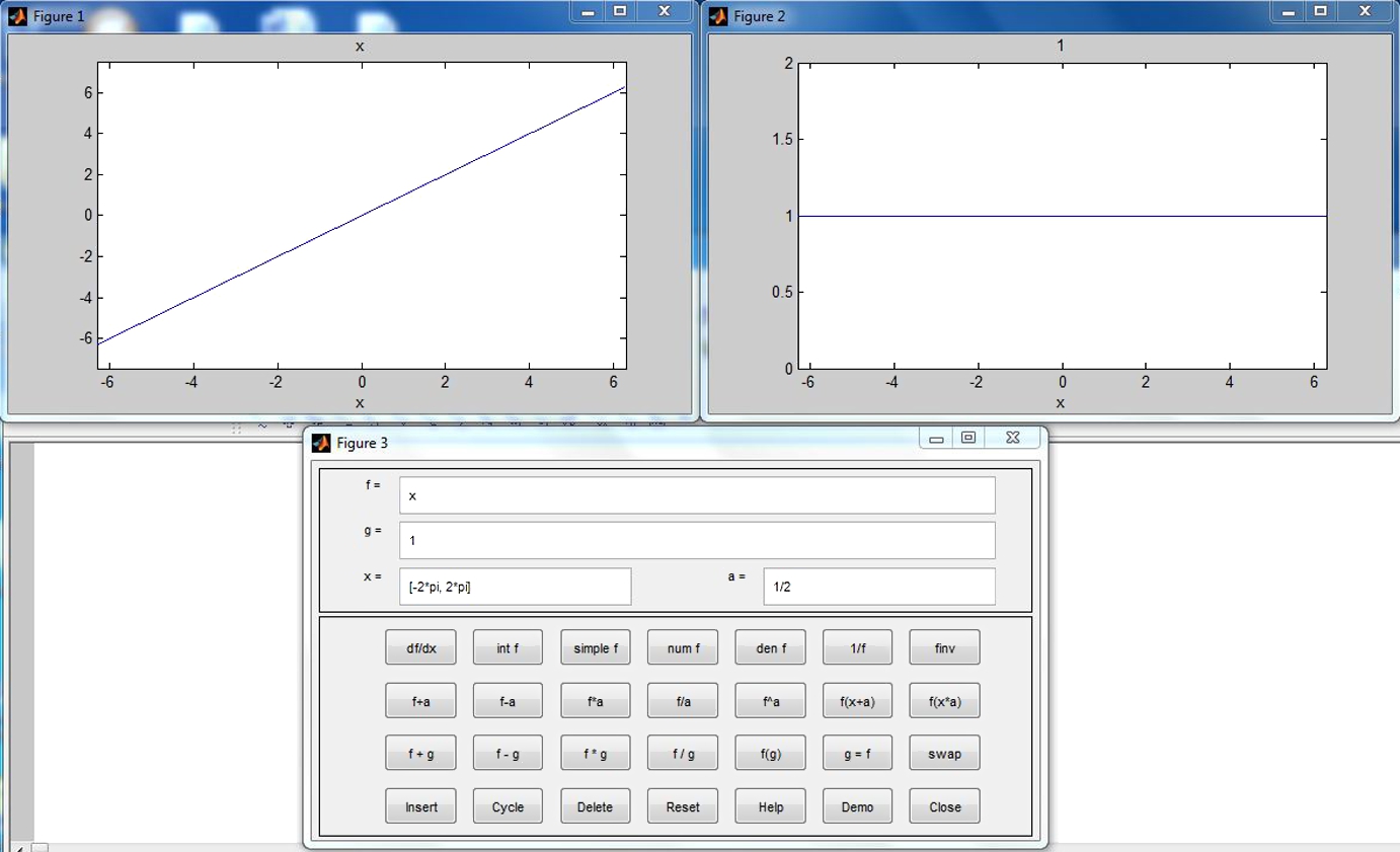
FIGURE 17.3 The function tool.

17.6.2. The MuPAD notebook^⁎ and Symbolic help

If you are interested in creating a notebook within MATLAB to examine a subject under investigation that requires symbolic among other tools to study, then the MuPAD notebook environment may be of interest. To open a new notebook type the following command in the Command Window and execute it.

>> mupad

The window illustrated in Figure 17.4 is opened. Examine the tools on the tool bar to learn how to input text as well as enter commands that allow you to execute Symbolic commands within this notebook environment.

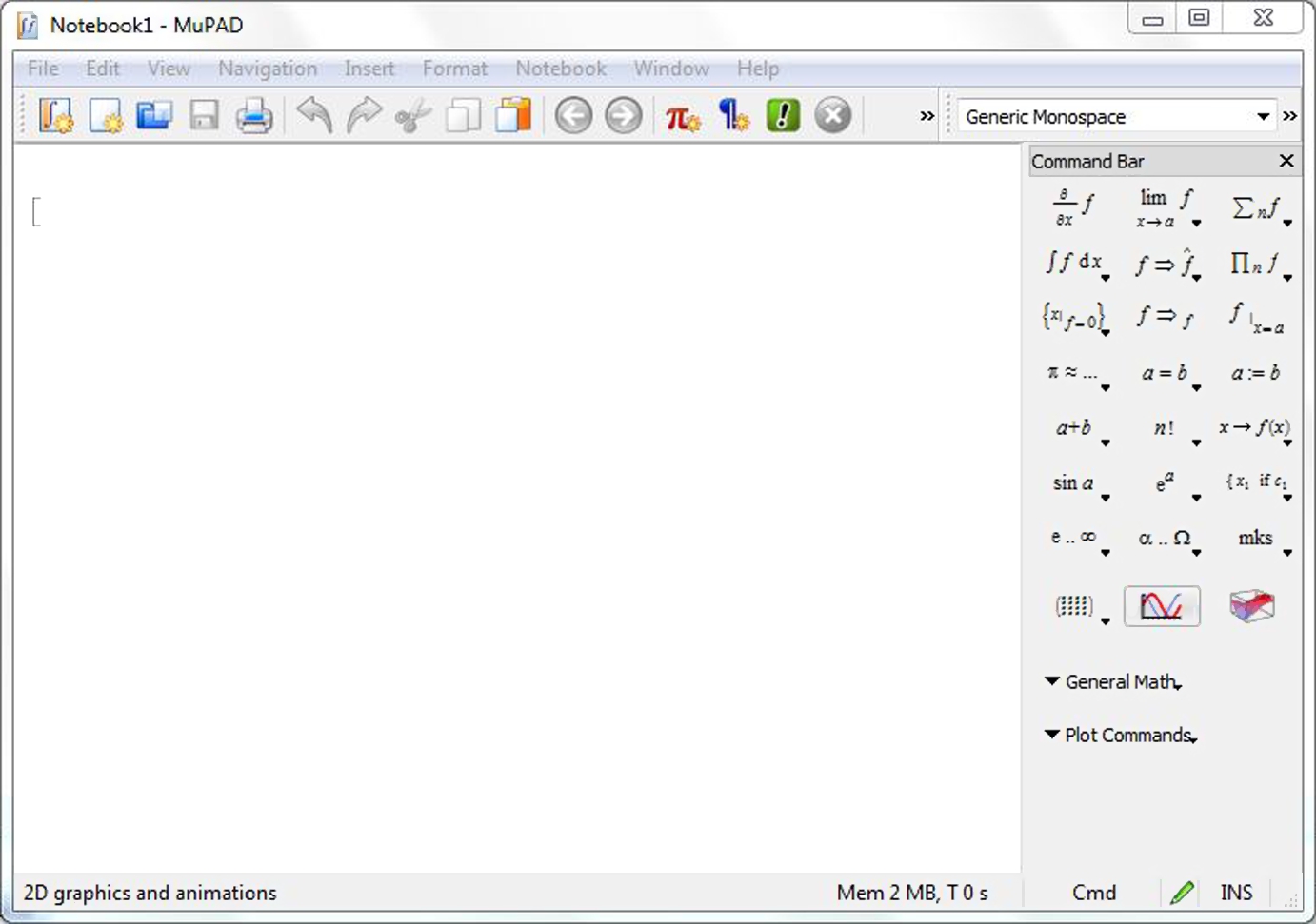
FIGURE 17.4 The notebook tool.

Finally, to get help on using mupad and other features of the Symbolic tools click the circled question mark, ‘?’, just below the word “Help” on the top tool bar. This opened the help window illustrated in Figure 17.5. To get to the Symbolics help click on Symbolic Math Toolbox in the contents palette. The information in the right hand pane will change to the information in Figure 17.6. Note that there are examples, help for MuPAD and demos that are quite useful.

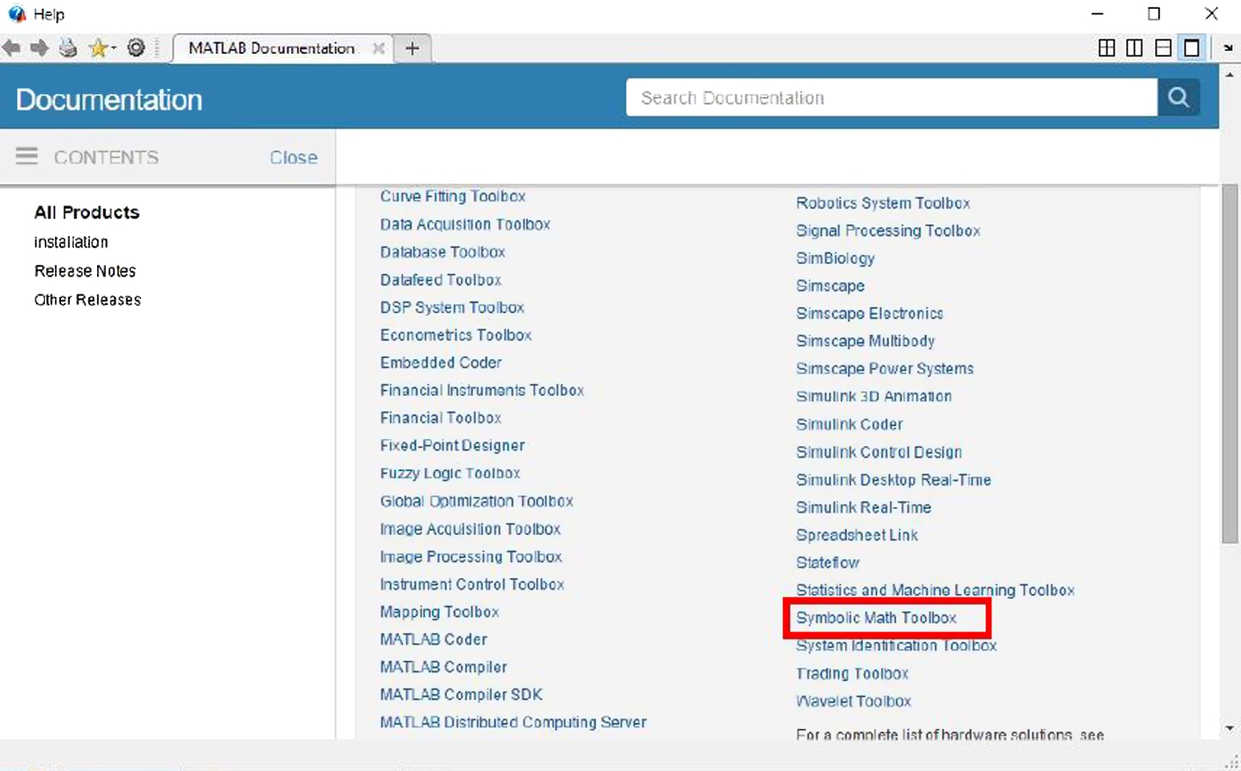
FIGURE 17.5 The MATLAB help documents: Click item in red box on the list of tools.

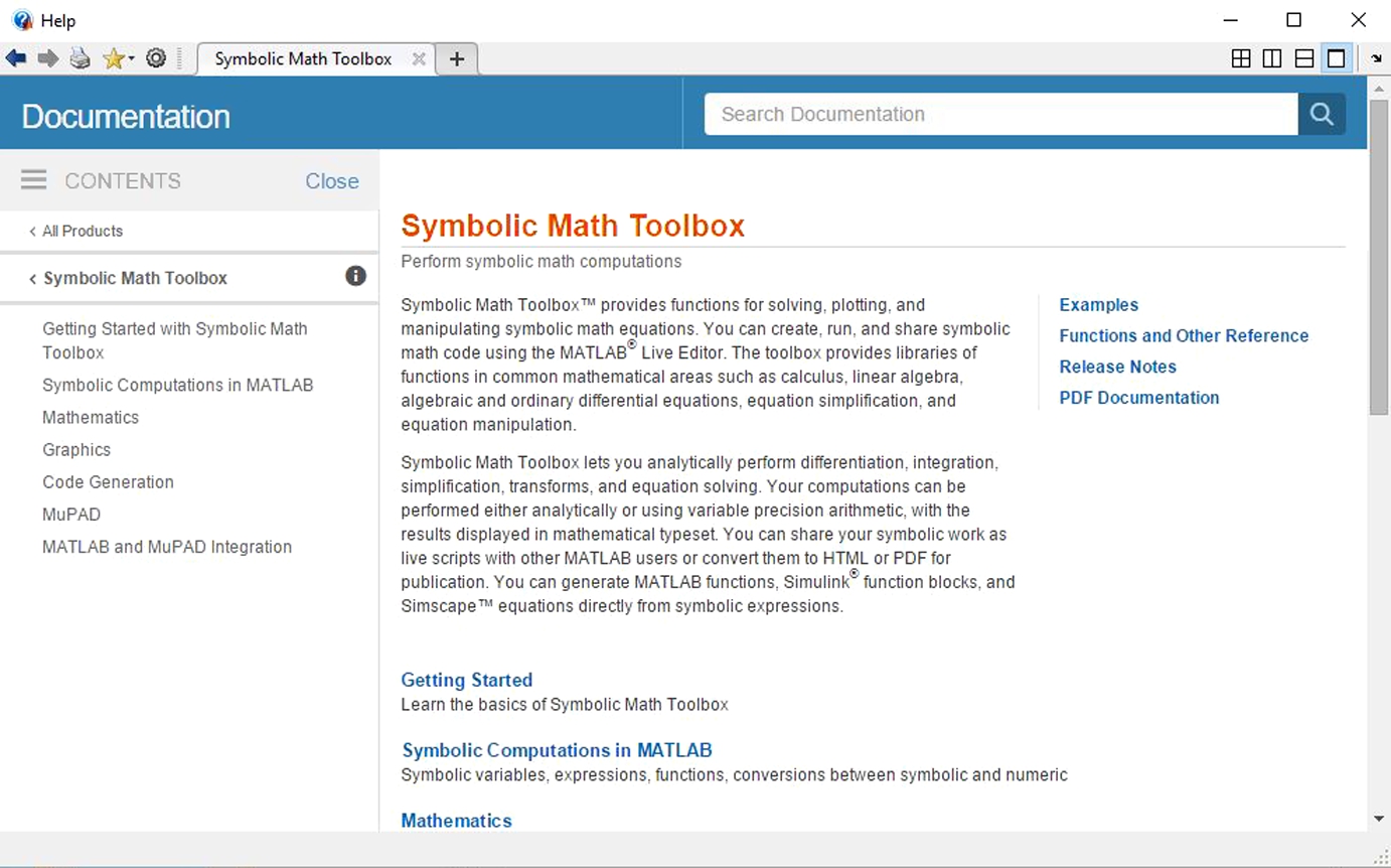
FIGURE 17.6 The help documents on the Symbolic tools.

Exercises

17.1 Find the derivatives of , and .

17.2 Integrate the function from to .