Software Engineering: A Methodical Approach (2014)
PART D. Software Development
Chapter 16. Software Economics
Software economics was first introduced in chapter 3 (section 3.7) though not by that term. At that time, we were discussing the feasibility of the software engineering project. After reading chapter 3, one may get the impression that software cost is equal to development cost. In this chapter, you will see that the two are often different; that development cost is just one component of software cost; and that there are other factors. You will also see that determination of software cost, software price and software value are difficult issues that continue to be the subject of research and further refinement. The chapter proceeds under the following captions:
· Software Cost versus Software Price
· Software Value
· Assessing Software Productivity
· Estimation Techniques for Engineering Cost
· Summary and Concluding Remarks
16.1 Software Cost versus Software Price
There are few cases where software cost is the same as software price; in most cases, they are different. Let us examine both.
16.1.1 Software Cost
As mentioned in chapter 3 (section 3.7.4), there are many components that go into the cost of developing a software system. These cost components are summarized in Figure 16-1.
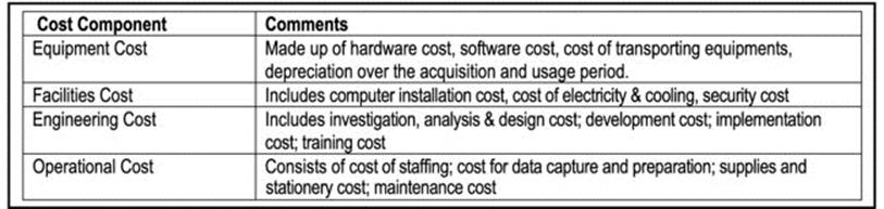
Figure 16-1. Software Engineering Cost Components
Software engineering is a business as well as an applied science. The business approach that many organizations employ is simply to put a price tag on each of these components based on experience as well as business policies: The equipment cost, facilities cost and operational cost will continue to remain purely business issues. The standard business approach for determining the engineering cost is to multiply the organization’s prescribed hourly rate by the estimated number of hours required for the project. However, as you will see later, there have been efforts to apply more scientific and objective techniques to the evaluating engineering cost through the exploration of deterministic models.
16.1.2 Software Price
Determining the software cost is important but it does not complete the software evaluation process. We must also determine the software (selling) price. Naturally, the biggest contributor to software price is software cost. Three scenarios are worth noting:
· If your organization is a software engineering firm and/or the product is to be marketed, then determining a selling price that consumers will pay for the product is critical. In this case, the price may be significantly discounted since software cost can be recovered from multiple sales.
· If your organization is not a software engineering firm and/or the product will not be marketed to the consuming public, then the software price is likely to be high, since its cost cannot be recovered from sale. In this case, the minimum price is the software cost.
· If your organization is a software engineering firm contracted to build a product exclusively for another organization, then the software price is likely to be high, since the software engineering firm must recover its costs and make a profit.
Figure 16-2 summarizes some of the main factors affecting software pricing. Please note that there may be other factors that affect the pricing of the software (for instance other quality factors). The intent here is to emphasize that pricing a software system is not a straightforward or trivial matter.
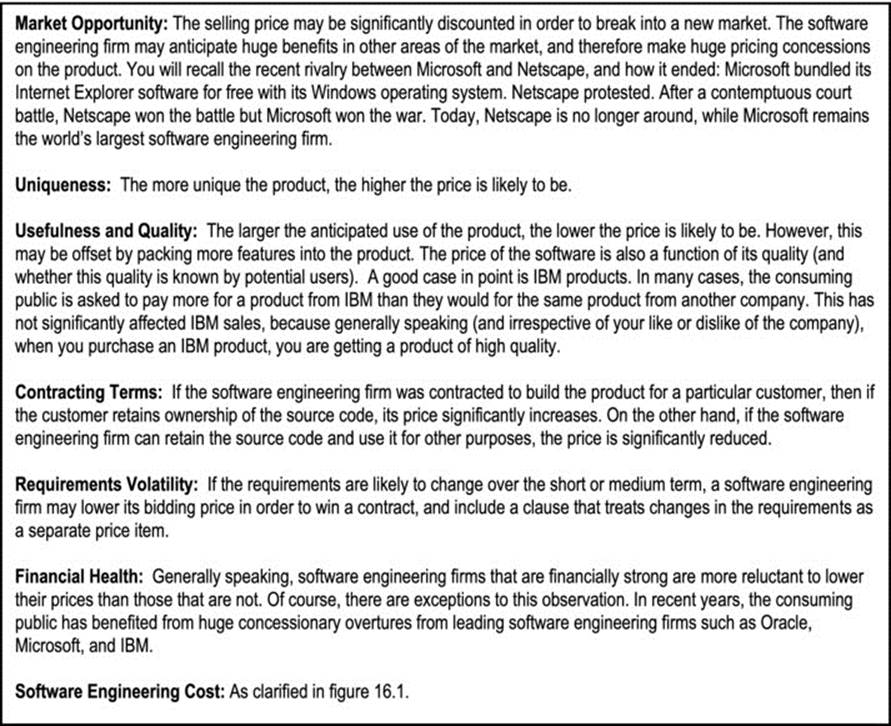
Figure 16-2. Some Factors Affecting Software Pricing
16.2 Software Value
The value of a software system may be different from the price. Whether your organization intends to market the software or not, it is often useful to place a value on the product, for the following reasons:
· If the product is being marketed, placing a value on it can provide a competitive advantage to the host organization (i.e. the organization that owns the product) if the value is significantly more than the price. The host organization can then use this as marketing advantage to appear generous to its prospective consumers.
· If the product is being kept by the host organization, then having a value that is significantly higher than its price/cost makes the acquisition more justifiable.
· Whatever the situation, it makes sense to place a value on the product from an accounting point of view.
The big question is, how do we place a value on a software product? There is no set formula or method for answering this question; therefore we resort to estimation techniques. A common sense approach is to assume that software value is a function of any or each of the following:
· Software cost
· Productivity brought to the organization (and how this translates to increased profit)
· Cost savings brought to the organization
In the end, determining a value for the software system is a management function that is informed by software engineering. For this reason, we will examine some of the estimation techniques that are available (section 16.4). Before doing so, we will take a closer look at evaluating software productivity.
16.3 Evaluating Software Productivity
There are two approaches to assessing software productivity. One is to concentrate on the effort of the software engineer(s). The other is to concentrate on the added value to the enterprise due to the software product. Most of the proposed models tend to concentrate on the former approach. In keeping with the theme of the text, and in the interest of comprehensive coverage, we will examine both approaches.
A common method of assessment of software productivity is to treat it as a function of the productivity contribution of the software product, and the collective engineering effort. Two common types of metrics have been discussed in [Sommerville, 2006]. They are size-related metrics andfunction-related metrics. A third approach is a value-added metrics; it attempts to determine and associated value added by a software system to an organization. A brief discussion of each approach follows.
16.3.1 Size-related Metrics
Size-related methodologies rely on the software size as the main determinant of productivity evaluation. Common units of measure are the number of lines of source code, the number of object code instructions, and the number of pages of system documentation. To illustrate, a size-related metric may compute a software productivity index for a project, based on the formulae in Figure 16-3.
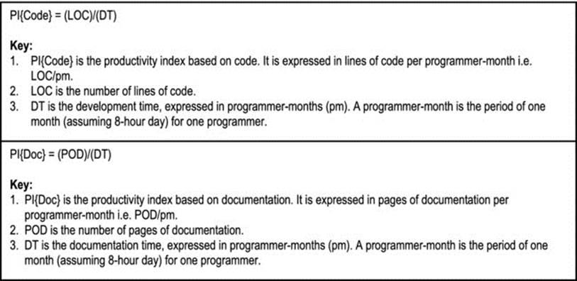
Figure 16-3. Formulae for Size-related Metrics
Associated with this approach are the following caveats:
· If different programming languages are used on the same project, then making a single calculation for PI{Code} would be incorrect, since the level of productivity varies from one software development environment to another. A more prudent approach would be to calculate the PI{Code} for each language and take a weighted average.
· Most of the documented size-related metrics concentrate on lines of code, with scant or no regard for documentation. This plays squarely into the fallacy that software engineering is equivalent to programming. The lower half of figure 16-3 has been added to provide balance and proper perspective to the analysis. If as proposed by this course, more effort ought to be placed on software design than on software development, and that the latter should be an exciting and enjoyable follow-up of the former, then any evaluation of software cost or productivity should reflect that perspective.
The main problem with this model is that it does not address the important matter of software quality. What if the software product and documentation are both voluminous due to faulty design? The model does not address this concern.
16.3.2 Function-related Metrics
Function-related methodologies rely on the software functionality as the main determinant of productivity evaluation. The common unit of measure for these methodologies is the function-points (FP) per programmer-month (a programmer-month is the time taken by one programmer for one month, assuming a normal work week of 40 hours). The number of function points for each program is estimated based on the following:
· External inputs and outputs
· User interactions
· External inquiries
· Files used
Additionally, a complexity weighting factor (originally in the range of 3 to 15) is applied to each program. Next, an unadjusted function-point count (UFC) is calculated by cumulating the initial function-points count times the weight, for each component:

Next, complexity factors are assigned for the project based on other factors such as code reuse, distributed processing, etc. The UFC is then multiplied to this/these other complexity factor(s) to yield an adjusted function-point count (AFC). Finally, the productivity index is calculated.
Figure 16-4 summarizes the essence of the approach. Associated with this approach are the following caveats:
· The approach is language independent.
· It is arguable as to how effective this approach is for event-driven systems and systems developed in the OO paradigm. For this reason, object-points have been proposed to replace function points for OO systems. We will discuss object-points later (section 16.4.3).
· The approach is heavily biased towards software development rather than the entire software engineering life cycle.
· The approach is highly subjective. The function-points, weights, and complexity factors are all subjectively assigned by the estimator.
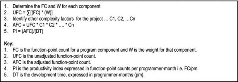
Figure 16-4. Calculations for Function-related Metrics
The matter of software quality still remains a concern, though to some extent, it has been addressed in the software’s functionality. Indeed, it can be argued that to some extent, a software system’s functionality is determined by the quality of the software design.
16.3.3 Assessment Based on Value Added
There is much work in the area of value-added assessment in the field of education as well as other more traditional engineering fields. Unfortunately, the software engineering industry is somewhat lacking in this area. In value-added software assessment, we ask and attempt to obtain the answer to the question, what value has been added to the organization by introduction of a software system or a set of software systems? In pursuing an accurate answer to this question, there are two alternatives that are available to the software engineer:
· Evaluate the additional revenue that the software system facilitated.
· Evaluate the reduced expenditure that the software system has contributed to.
These alternatives are by no means mutually exclusive; in fact, in many instances they both apply. One way to conduct the analysis is to estimate the useful economic life of the software system, and compute the above-mentioned values over that period. In hindsight, this may be challenging, but by no means insurmountable. However, the reality is, in most cases, it is desirable to conduct this analysis prior to the end of the economic life of the system. Moreover, in many cases, this analysis is required up front, as part of the feasibility study for a software engineering venture (review section 3.7).
Figure 16-5 provides two formulae that may be employed in estimating the value added by a software system. The first facilitates a crude estimate, assuming that interest rates remain constant over the period of analysis (of course, this is not practical, which is why it’s described as a crude estimate). Since this approach involves taking the difference between the value added and the acquisition cost, you may call it the difference method. The second formula computes the net present value (NPV), with due consideration to interest rates; it is considered a more realistic estimate. The simple adjustment to be made here is to ensure that the cash flow per annum includes additional revenue due to the system as well as reduced expenditure due to the system.
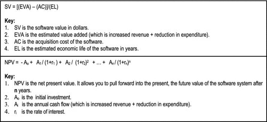
Figure 16-5. Estimating Software Value-added
16.4 Estimation Techniques for Engineering Cost
In the foregoing discussion, the importance of the engineering cost and the challenges to accurately determining it were emphasized. In section 16.1, it was mentioned that the standard business approach to estimating engineering cost is to multiply the estimated project duration (in hours) by the organization’s prescribed hourly engineering rate. In this section, we will examine the engineering cost a bit closer, and look at other models for cost estimation.
Our discussion commences with the work of Barry Boehm [Boehm, 2002]. According to the Boehm model for cost estimation, there are five approaches to software cost estimation (more precisely, the software engineering cost estimation) as summarized below:
· Algorithmic Cost Modeling: The cost is determined as a function of the effort.
· Expert Judgment: A group of experts assess the project and estimate its cost.
· Analogy: The project is compared to some other completed project in the same application domain, and its cost is estimated.
· Parkinson’s Law: The project cost is based on convenience factors such as available resources, and time horizon.
· Pricing Based on Consumer: The project is assigned a cost based on the consumer’s financial resources, and not necessarily on the software requirements.
Obviously, the latter four proposals are highly subjective and error-prone; they will not be explored any further. The algorithmic approach has generated much interest and subsequent proposals over the past twenty-five years, some of which have been listed for recommended readings.
16.4.1 Algorithmic Cost Models
Algorithmic cost models assume that project cost is a function of other project factors such as size, number of software engineers, and possibly others. As such, each cost model uses a mathematical formula to compute an index for the software engineering effort (E). The cost is then determined based on the evaluation of the effort. Figure 16-6 outlines the typical cost model.
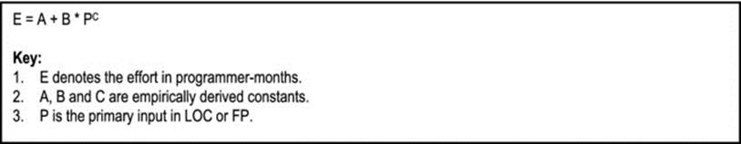
Figure 16-6. Typical Cost Model
By way of observation, the exponent C typically lies in the range {0.8 .. 1.5}. The constants A, B, and C are called adjustment parameters, and they are determined by project characteristics (such as complexity, experience of the project team members, the development environment, etc.).
Pressman [Pressman, 2005] lists a number of specific cases-in-point of this cost model, such as:
· E = 5.2 * (KLOC)0.91 … the Watson-Felix model
· E = 5.5 + 0.73 * (KLOC)1.16 … the Bailey-Basili model
· E = 3.2 * (KLOC)1.05 … the COCOMO Basic model
· E = 5.288 * (KLOC)1.047 … the Doty model for KLOC > 9
· E = -91.4 + 0.355 * (FP) … the Albrecht & Gaffney model
· E = -37 + 0.96 * (FP) … the Kemerer model
· E = -12.88 + 0.405 * (FP) … the small project regression model
![]() Note In the above examples, the acronym KLOC means thousand lines of code.
Note In the above examples, the acronym KLOC means thousand lines of code.
16.4.2 The COCOMO Model
Boehm first proposed the Constructive Cost Model (COCOMO) in 1981, and since then it has matured to the status of international fame. The basic model was of the form
![]()
Boehm used a three-mode approach, as follows (Figure 16-7 provides the formula used for each model):
· Organic Mode — for relatively simple projects.
· Semi-detached Mode — for intermediate-level projects with team members of limited experience.
· Embedded Mode — for complex projects with rigid constraints.
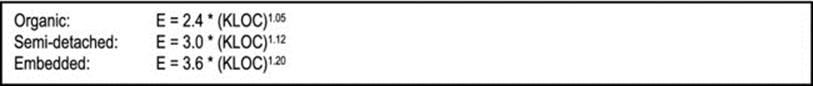
Figure 16-7. COCOMO Formulae
The original COCOMO model was designed based on traditional procedural programming in languages such as C, Fortran, etc. Additionally, most (if not all) software engineering projects were pursued based on the waterfall model. The next subsection discusses Boehm’s revision of this basic model.
16.4.3 The COCOMO II Model
Software engineering has changed significantly since the basic COCOMO model was first introduced. At the time of introduction, OOM was just an emerging idea, and most software engineering projects followed the waterfall model. In contrast, today, most software engineering projects are pursued in the OO paradigm, and the waterfall model has given way to more flexible, responsive approaches (review chapter 1). In 1997, Boehm and his colleagues introduced a revised COCOMO II model to facilitate the changes in the software engineering paradigm.
The COCOMO II model is more inclusive, and receptive to OO software development tools. It facilitates assessment based on the following:
· Number of lines of source code
· Number of object-points or function-points
· Number of lines of code reused or generated
· Number of application points
The changes relate to application points and code reuse/generation — features of contemporary OO software development tools. We will address both in what is called the application composition model. Two other sub-models of COCOMO II are the early design model and the post-architecture model.
Application Composition Model
In the application composition model, we are interested in object points (OP) as opposed to function points (FP). The model can be explained in seven steps as summarized below:
1. The number of object points in a software system is the weighted estimate of the following:
· The number of separate screens displayed
· The number of reports produced
· The number of components that must be developed to supplement the application
2. Each object instance is classified into one of three complexity levels — simple, medium or difficult — according to the schedule in Figure 16-8.
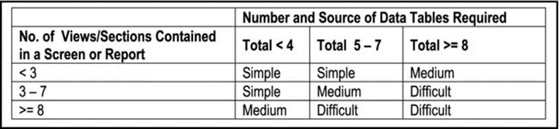
Figure 16-8. Object Instance Classification Guide
3. The number of screens, reports, and components are weighted according to the schedule in figure 16-9. The weights actually represent the relative effort required to implement an instance of that complexity level.
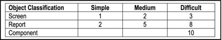
Figure 16-9. Complexity Weights for Object Classifications
4. Determine the object point count (OPC) by multiplying the original number of object instances by the weighting factor, and summing to obtain the total OPC. Figure 16-10a clarifies the calculation and Figure 16-10b provides an illustration.
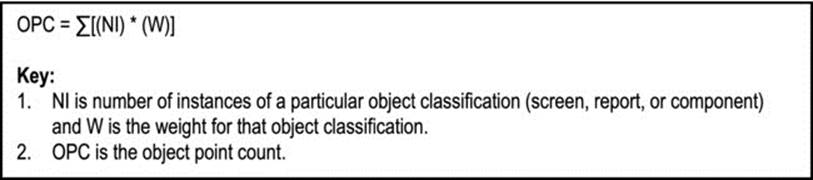
Figure 16-10a. Calculating the OPC
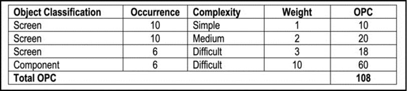
Figure 16-10b. Illustrating Calculation of the OPC
5. Calculate the number of object points (NOP) by adjusting the OPC based on the level of code reuse in the application:
![]()
6. Determine a productivity rate (PR) for the project, based on the schedule of Figure 16-11. Note that the schedule that it is in the project’s best interest to have a project team of very talented and experienced software engineers, and to use the best software development that is available.
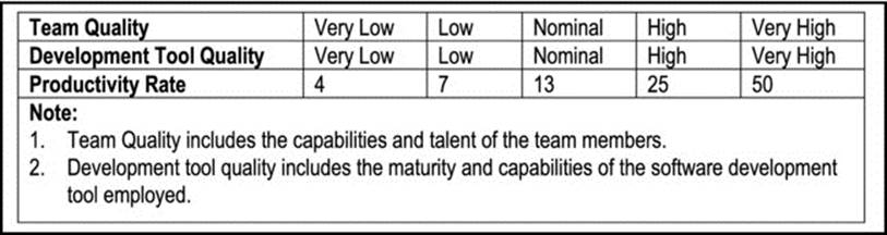
Figure 16-11. Productivity Rate Schedule
7. Compute the effort (E) via the formula
![]()
Figure 16-12 summarizes the steps in the application composition model. With practice on real projects, you will become more comfortable with this cost estimation technique. The important thing to remember about the model is that the software cost is construed to be a function of the engineering effort, and the complexity of the software.
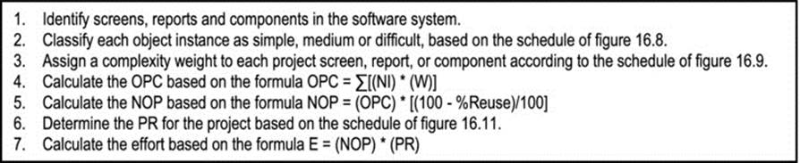
Figure 16-12. Summary of the Application Composition Model
Early Design Model
The early design model is recommended for the early stages the software engineering project (after the requirements specification has been prepared). A full discussion of the approach will not be conducted here, but a summary follows.
The formula used for calculating effort is
![]()
As clarified earlier, B and C are constants, and P denotes the primary input (estimated LOC or FP). Based on Boehm’s experiments, A is recommended to be 2.94, and C may vary between 1.1 and 1.24. The EAF is a multiplier that is determined based on the following seven factors (called cost drivers). In the interest of clarity, the originally proposed acronyms have been changed:
· Product Reliability and Complexity (PRC)
· Required Reuse (RR)
· Platform Difficulty (PD)
· Personnel Capability (PC)
· Personnel Experience (PE)
· Facilities (F)
· Schedule (S)
![]()
Post-Architecture Model
The post-architecture model is the most detailed of the COCOMO II sub-models. It is recommend for use during actual development, and subsequent maintenance of the software system (chapter 18 discusses software maintenance).
The formula used for calculating effort is of identical form as for the early design model:
![]()
In this case, B is empirically recommended to be 2.55 and C is calculated via the formula

The criteria (also called scale factors) used to assign capability weights (CW) about the project and the project team are as follows:
· Precedence: Does the organization have prior experience working on a similar project?
· Development Flexibility: The degree of flexibility in the software development process.
· Architecture/Risk Resolution: How much risk analysis has been done, and what steps have been taken to lessen of eliminate these risks?
· Team Cohesion: How cohesive is the team?
· Process Maturity: What is the process maturity of the organization? How capable is it in successfully pursuing this project?
Figure 16-13 provides the recommended schedule for determining the capability weights for these criteria. As can be seen from the figure, the weights range from 0 (extra high) to 6 (very low).
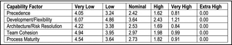
Figure 16-13. Capability Weights Schedule
The EAF is determined from a much wider range of factors than the early design model. Here, there are seventeen factors (cost drivers). Figure 16-14 lists these cost drivers along with their assigned ratings. In the interest of clarity, the original acronyms have been changed. The EAF is the product of these cost multipliers.
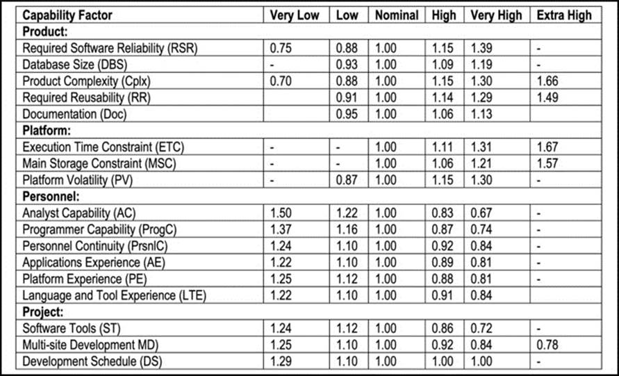
Figure 16-14. Post-Architecture Cost Drivers Schedule
You have no doubt observed that this is quite a complex cost model. It must be emphasized that in order to be of any use, the model must be calibrated to suit the local situation, based on local history. Moreover, there is considerable scope for uncertainty in estimation of values for the various factors. The model must therefore be used as a guideline, not a law cast in stone.
16.5 Summary and Concluding Remarks
Let us summarize what we have discussed in this chapter:
· Software cost is comprised of equipment cost, facilities cost, engineering cost and operational cost. Equipment cost, facilities cost, and operational cost, are determined by following standard business procedures. Engineering cost may be determined using standard business procedures also, but in software engineering, we are also interested in fine-tuning the estimation of this cost component by exploring more deterministic models.
· Software price is influenced by factors including (but not confined to) software cost, market opportunity, uniqueness, usefulness and quality, contracting terms, requirements volatility, and financial health of the organization that owns the product.
· Software value is influenced by software cost, productivity brought the organization, and cost savings brought to the organization.
· Software productivity may be evaluated based on the software engineering effort employed in planning and constructing the product, or based on the value added to the organization. Two metrics used for evaluating the engineering effort are the size-based metrics, and the function-based metrics. Two methods for evaluating value added are the difference method, and the NPV analysis method.
· The size-based metrics estimate productivity based on the number of lines of code and pages of documentation of the software.
· Function-based metrics estimate productivity based on the number of function-points of the software.
· Value-added metrics attempt to estimate the value added to the organization by the software.
· Techniques for estimating engineering costs include algorithmic cost modeling, expert judgment, analogy, Parkinson’s Law, and pricing based on consumer. Algorithmic cost modeling presents much research interest in software engineering.
· The typical formula for evaluating engineering effort in algorithmic cost modeling is E = A + B * PC.
· The COCOMO model uses three derivations of the basic algorithmic cost modeling formula. The model relates to traditional systems developed in the FO paradigm.
· The COCOMO II model is a revision of the basic COCOMO model, to facilitate more contemporary software systems developed in the OO paradigm. It includes an application component model, an early design model, and a post-architecture model.
· The application composition model outlines a seven-step approach for obtaining an evaluation of the engineering effort of the software system. This is summarized in Figure 16-12.
· The early design model uses an adjusted formula for evaluating the engineering effort. The formula is E = B * PC * (EAF), and certain precautions must be followed when using it.
· The post-architecture model uses the same formula E = B * PC * (EAF); however, the precautions to be followed are much more elaborate.
We have covered a lot of ground towards building software systems of a high quality. The deliverable that comes out of the software development phase is the actual product! It is therefore time to discuss implementation and maintenance. The next three chapters will do that.
16.6 Review Questions
1. What is the difference between software cost and software price?
2. What are the components of software cost? What are the challenges to determining software cost?
3. State and briefly discuss the main factors that influence software price?
4. How is software value determined? What are the challenges to determining software value?
5. State three approaches to evaluating software productivity. For each approach, outline a methodology, and briefly highlight its limitations.
6. Identify Boehm’s five approaches to software cost estimation. Which approach provides the most interest for software engineers?
7. Describe the basic algorithmic cost model that many software costing techniques employ.
8. Describe the COCOMO II model.
9. Choose a software engineering project that you are familiar with.
a. Using the COCOMO II Application Composition Model, determine an evaluation of the engineering effort of the project.
b. Using the COCOMO II Early Design Model, determine an evaluation of the engineering effort of the project.
c. Using the COCOMO II Post-Architecture Model, determine an evaluation of the engineering effort of the project.
d. Compare the results obtained in each case.
16.7 References and/or Recommended Reading
[Albrecht, 1979] Albrecht, A. J. “Measuring Application-Development Productivity.” AHARE/GUIDE IBM Application Development Symposium. 1979. See chapter 26.
[Boehm, 1981] Boehm, BarryW. Software Engineering Economics. Englewood Cliffs, NJ: Prentice Hall, 1981.
[Boehm et. al., 1997] Boehm, Barry W., C. Abts, B. Clark, and S. Devnani-Chulani. COCOMO II Model Definition Manual. Los Angeles, CA: University of Southern California, 1997.
[Boehm, 2002] Boehm, Barry W., et. al. COCOMO II. http://sunset.usc.edu/research/COCOMOII (accessed July 2006).
[Fenton, 1997] Fenton, Norman E. and Shari L. Pfleeger. Software Metrics: A Rigorous and Practical Approach. Boston, MA: PWS Publishing, 1997.
[Humphrey, 1990] Humphrey, Watts S. Managing the Software Process. Reading, MA: Addison-Wesley Publishing, 1990.
[Jones, 1997] Jones, Capers. Applied Software Measurement: Assuring Productivity and Quality 2nd ed. New York, NY: McGraw-Hill, 1997.
[MacDonell, 1994] MacDonell, Stephen G. “Comparative Review of Functional Complexity Assessment Methods for Effort Estimation.” BCS/IEE Software Engineering Journal 9(3), 1994. pp.107–116.
[Pressman, 2005] Pressman, Roger. Software Engineering: A Practitioner’s Approach 6th ed. Crawfordsville, IN: McGraw-Hill, 2005. See chapter 23.
[Putnam, 1992] Putnam, Lawrence H. and Ware Myers. Measures for Excellence: Reliable Software on time, within Budget. Englewood Cliffs, NJ: Yourdon Press, 1992.
[Sommerville, 2006] Sommerville, Ian. Software Engineering 8th ed. Reading, MA: Addison-Wesley, 2006. See chapter 26.