Mining the Social Web (2014)
Part I. A Guided Tour of the Social Web
Chapter 5. Mining Web Pages: Using Natural Language Processing to Understand Human Language, Summarize Blog Posts, and More
This chapter follows closely on the heels of the chapter before it and is a modest attempt to introduce natural language processing (NLP) and apply it to the vast source of human language[17] data that you’ll encounter on the social web (or elsewhere). The previous chapter introduced some foundational techniques from information retrieval (IR) theory, which generally treats text as document-centric “bags of words” (unordered collections of words) that can be modeled and manipulated as vectors. Although these models often perform remarkably well in many circumstances, a recurring shortcoming is that they do not maximize cues from the immediate context that ground words in meaning.
This chapter employs different techniques that are more context-driven and delves deeper into the semantics of human language data. Social web APIs that return data conforming to a well-defined schema are essential, but the most basic currency of human communication is natural language data such as the words that you are reading on this page, Facebook posts, web pages linked into tweets, and so forth. Human language is by far the most ubiquitous kind of data available to us, and the future of data-driven innovation depends largely upon our ability to effectively harness machines to understand digital forms of human communication.
NOTE
It is highly recommended that you have a good working knowledge of the content in the previous chapter before you dive into this chapter. A good understanding of NLP presupposes an appreciation and working knowledge of some of the fundamental strengths and weaknesses of TF-IDF, vector space models, and so on. In that regard, this chapter and the one before it have a somewhat tighter coupling than most other chapters in this book.
In the spirit of the prior chapters, we’ll attempt to cover the minimal level of detail required to empower you with a solid general understanding of an inherently complex topic, while also providing enough of a technical drill-down that you’ll be able to immediately get to work mining some data. While continuing to cut corners and attempting to give you the crucial 20% of the skills that you can use to do 80% of the work (no single chapter out of any book—or small multivolume set of books, for that matter—could possibly do the topic of NLP justice), the content in this chapter is a pragmatic introduction that’ll give you enough information to do some pretty amazing things with the human language data that you’ll find all over the social web. Although we’ll be focused on extracting human language data from web pages and feeds, keep in mind that just about every social website with an API is going to return human language, so these techniques generalize to just about any social website.
NOTE
Always get the latest bug-fixed source code for this chapter (and every other chapter) online at http://bit.ly/MiningTheSocialWeb2E. Be sure to also take advantage of this book’s virtual machine experience, as described in Appendix A, to maximize your enjoyment of the sample code.
Overview
This chapter continues our journey in analyzing human language data and uses arbitrary web pages and feeds as a basis. In this chapter you’ll learn about:
§ Fetching web pages and extracting the human language data from them
§ Leveraging NLTK for completing fundamental tasks in natural language processing
§ Contextually driven analysis in NLP
§ Using NLP to complete analytical tasks such as generating document abstracts
§ Metrics for measuring quality for domains that involve predictive analysis
Scraping, Parsing, and Crawling the Web
Although it’s trivial to use a programming language or terminal utility such as curl or wget to fetch an arbitrary web page, extracting the isolated text that you want from the page isn’t quite as trivial. Although the text is certainly in the page, so is lots of other boilerplate content such as navigation bars, headers, footers, advertisements, and other sources of noise that you probably don’t care about. Hence, the bad news is that the problem isn’t quite as simple as just stripping out the HTML tags and processing the text that is left behind, because the removal of HTML tags would have done nothing to remove the boilerplate itself. In some cases, there may actually be more boilerplate in the page that contributes noise than the signal you were looking for in the first place.
The good news is that the tools for helping to identify the content you’re interested in have continued to mature over the years, and there are some excellent options for isolating the material that you’d want for text-mining purposes. Additionally, the relative ubiquity of feeds such as RSS and Atom can often aid the process of retrieving clean text without all of the cruft that’s typically in web pages, if you have the foresight to fetch the feeds while they are available.
NOTE
It’s often the case that feeds are published only for “recent” content, so you may sometimes have to process web pages even if feeds are available. If given the choice, you’ll probably want to prefer the feeds over arbitrary web pages, but you’ll need to be prepared for both.
One excellent tool for web scraping (the process of extracting text from a web page) is the Java-based boilerpipe library, which is designed to identify and remove the boilerplate from web pages. The boilerpipe library is based on a published paper entitled “Boilerplate Detection Using Shallow Text Features,” which explains the efficacy of using supervised machine learning techniques to bifurcate the boilerplate and the content of the page. Supervised machine learning techniques involve a process that creates a predictive model from training samples that are representative of its domain, and thus, boilerpipe is customizable should you desire to tweak it for increased accuracy.
Even though the library is Java-based, it’s useful and popular enough that a Python package wrapper called python-boilerpipe is available.. Installation of this package is predictable: use pip install boilerpipe. Assuming you have a relatively recent version of Java on your system, that’s all that should be required to use boilerpipe.
Example 5-1 demonstrates a sample script that illustrates its rather straightforward usage for the task of extracting the body content of an article, as denoted by the ArticleExtractor parameter that’s passed into the Extractor constructor. You can also try out a hosted version of boilerpipe online to see the difference between some of its other provided extractors, such as the LargestContentExtractor or DefaultExtractor.
There’s a default extractor that works for the general case, an extractor that has been trained for web pages containing articles, and an extractor that is trained to extract the largest body of text on a page, which might be suitable for web pages that tend to have just one large block of text. In any case, there may still be some light post-processing required on the text, depending on what other features you can identify that may be noise or require attention, but employing boilerpipe to do the heavy lifting is just about as easy as it should be.
Example 5-1. Using boilerpipe to extract the text from a web page
fromboilerpipe.extractimport Extractor
URL='http://radar.oreilly.com/2010/07/louvre-industrial-age-henry-ford.html'
extractor = Extractor(extractor='ArticleExtractor', url=URL)
print extractor.getText()
Although web scraping used to be the only way to fetch content from websites, there’s potentially an easier way to harvest content, especially if it’s content that’s coming from a news source, blog, or other syndicated source. But before we get into that, let’s take a quick trip down memory lane.
If you’ve been using the Web long enough, you may remember a time in the late 1990s when news readers didn’t exist. Back then, if you wanted to know what the latest changes to a website were, you just had to go to the site and see if anything had changed. As a result, syndication formats took advantage of the self-publishing movement with blogs and formats such as RSS (Really Simple Syndication) and Atom built upon the evolving XML specifications that were growing in popularity to handle content providers publishing content and consumers subscribing to it. Parsing feeds is an easier problem to solve since the feeds are well-formed XML data that validates to a published schema, whereas web pages may or may not be well formed, be valid, or even conform to best practices.
A commonly used Python package for processing feed, appropriately named feedparser, is an essential utility to have on hand for parsing feeds. You can install it with pip using the standard pip install feedparser approach in a terminal, and Example 5-2 illustrates minimal usage to extract the text, title, and source URL for an entry in an RSS feed.
Example 5-2. Using feedparser to extract the text (and other fields) from an RSS or Atom feed
importfeedparser
FEED_URL='http://feeds.feedburner.com/oreilly/radar/atom'
fp = feedparser.parse(FEED_URL)
for e infp.entries:
print e.title
print e.links[0].href
print e.content[0].value
HTML, XML, AND XHTML
As the early Web evolved, the difficulty of separating the content in a page from its presentation quickly became recognized as a problem, and XML was (in part) a solution. The idea was that content creators could publish data in an XML format and use a stylesheet to transform it into XHTML for presentation to an end user. XHTML is essentially just HTML that is written as well-formed XML: each tag is defined in lowercase, tags are properly nested as a tree structure, and tags are either self-closing (such as <br />), or each opening tag (e.g., <p>) has a corresponding closing tag (</p>).
In the context of web scraping, these conventions have the added benefit of making each web page much easier to process with a parser, and in terms of design, it appeared that XHTML was exactly what the Web needed. There was a lot to gain and virtually nothing to lose from the proposition: well-formed XHTML content could be proven valid against an XML schema and enjoy all of the other perks of XML, such as custom attributes using namespaces (a device that semantic web technologies such as RDFa rely upon).
The problem is that it just didn’t catch on. As a result, we now live in a world where semantic markup based on the HTML 4.01 standard that’s over a decade old continues to thrive, while XHTML and XHTML-based technologies such as RDFa remain on the fringe. (In fact, libraries such as BeautifulSoup are designed with the specific intent of being able to reasonably process HTML that probably isn’t well-formed or even sane.) Most of the web development world is holding its breath and hoping that HTML5 will indeed create a long-overdue convergence as technologies like microdata catch on and publishing tools modernize. The HTML article on Wikipedia is worth reading if you find this kind of history interesting.
Crawling websites is a logical extension of the same concepts already presented in this section: it typically consists of fetching a page, extracting the hyperlinks in the page, and then systematically fetching all of those pages that are hyperlinked. This process is repeated to an arbitrary depth, depending on your objective. This very process is the way that the earliest search engines used to work, and the way most search engines that index the Web still continue to work today. Although a crawl of the Web is far outside our scope, it is helpful to have a working knowledge of the problem, so let’s briefly think about the computational complexity of harvesting all of those pages.
In terms of implementing your own web crawl, should you ever desire to do so, Scrapy is a Python-based framework for web scraping that serves as an excellent resource if your endeavors entail web crawling. The actual exercise of performing a web crawl is just outside the scope of this chapter, but the Scrapy documentation online is excellent and includes all of the tutelage you’ll need to get a targeted web crawl going with little effort up front. The next section is a brief aside that discusses the computational complexity of how web crawls are typically implemented so that you can better appreciate what you may be getting yourself into.
NOTE
Nowadays, you can get a periodically updated crawl of the Web that’s suitable for most research purposes from a source such as Amazon’s Common Crawl Corpus, which features more than 5 billion web pages and checks in at over 81 terabytes of data!
Breadth-First Search in Web Crawling
NOTE
This section contains some detailed content and analysis about how web crawls can be implemented and is not essential to your understanding of the content in this chapter (although you will likely find it interesting and edifying). If this is your first reading of the chapter, feel free to save it for next time.
The basic algorithm for a web crawl can be framed as a breadth-first search, which is a fundamental technique for exploring a space that’s typically modeled as a tree or a graph given a starting node and no other known information except a set of possibilities. In our web crawl scenario, our starting node would be the initial web page and the set of neighboring nodes would be the other pages that are hyperlinked.
There are alternative ways to search the space, with a depth-first search being a common alternative to a breadth-first search. The particular choice of one technique versus another often depends on available computing resources, specific domain knowledge, and even theoretical considerations. A breadth-first search is a reasonable approach for exploring a sliver of the Web. Example 5-3 presents some pseudocode that illustrates how it works, and Figure 5-1 provides some visual insight into how the search would look if you were to draw it out on the back of a napkin.
Example 5-3. Pseudocode for a breadth-first search
Create an empty graph
Create an empty queue to keep track of nodes that need to be processed
Add the starting point to the graph as the root node
Add the root node to a queue for processing
Repeat until some maximum depth is reached or the queue is empty:
Remove a node from the queue
For each of the node's neighbors:
If the neighbor hasn't already been processed:
Add it to the queue
Add it to the graph
Create an edge in the graph that connects the node and its neighbor
We generally haven’t taken quite this long of a pause to analyze an approach, but breadth-first search is a fundamental tool you’ll want to have in your belt and understand well. In general, there are two criteria for examination that you should always consider for an algorithm: efficiency and effectiveness (or, to put it another way: performance and quality).
Standard performance analysis of any algorithm generally involves examining its worst-case time and space complexity—in other words, the amount of time it would take the program to execute, and the amount of memory required for execution over a very large data set. The breadth-first approach we’ve used to frame a web crawl is essentially a breadth-first search, except that we’re not actually searching for anything in particular because there are no exit criteria beyond expanding the graph out either to a maximum depth or until we run out of nodes. If we were searching for something specific instead of just crawling links indefinitely, that would be considered an actual breadth-first search. Thus, a more common variation of a breadth-first search is called a bounded breadth-first search, which imposes a limit on the maximum depth of the search just as we do in this example.
For a breadth-first search (or breadth-first crawl), both the time and space complexity can be bounded in the worst case by bd, where b is the branching factor of the graph and d is the depth. If you sketch out an example on paper, as in Figure 5-1, and think about it, this analysis quickly becomes more apparent.
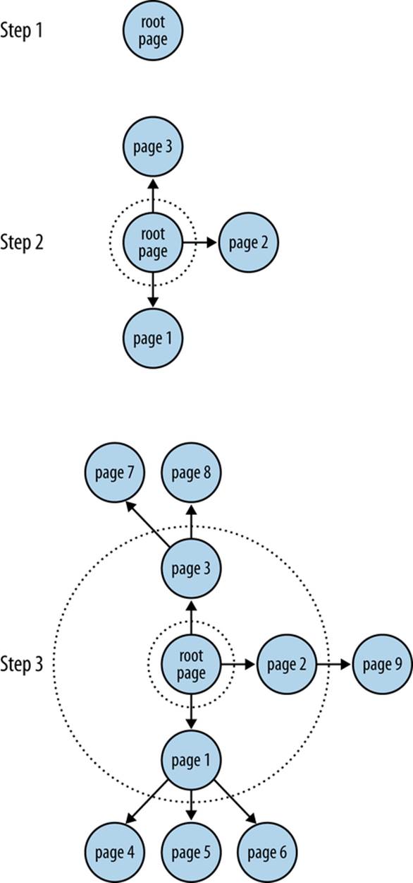
Figure 5-1. In a breadth-first search, each step of the search expands the depth by one level until a maximum depth or some other termination criterion is reached
If every node in a graph had five neighbors, and you only went out to a depth of one, you’d end up with six nodes in all: the root node and its five neighbors. If all five of those neighbors had five neighbors too and you expanded out another level, you’d end up with 31 nodes in all: the root node, the root node’s five neighbors, and five neighbors for each of the root node’s neighbors. Table 5-1 provides an overview of how bd grows for a few sizes of b and d.
Table 5-1. Example branching factor calculations for graphs of varying depths
|
Branching factor |
Nodes for depth = 1 |
Nodes for depth = 2 |
Nodes for depth = 3 |
Nodes for depth = 4 |
Nodes for depth = 5 |
|
2 |
3 |
7 |
15 |
31 |
63 |
|
3 |
4 |
13 |
40 |
121 |
364 |
|
4 |
5 |
21 |
85 |
341 |
1,365 |
|
5 |
6 |
31 |
156 |
781 |
3,906 |
|
6 |
7 |
43 |
259 |
1,555 |
9,331 |
Figure 5-2 provides a visual for the values displayed in Table 5-1.
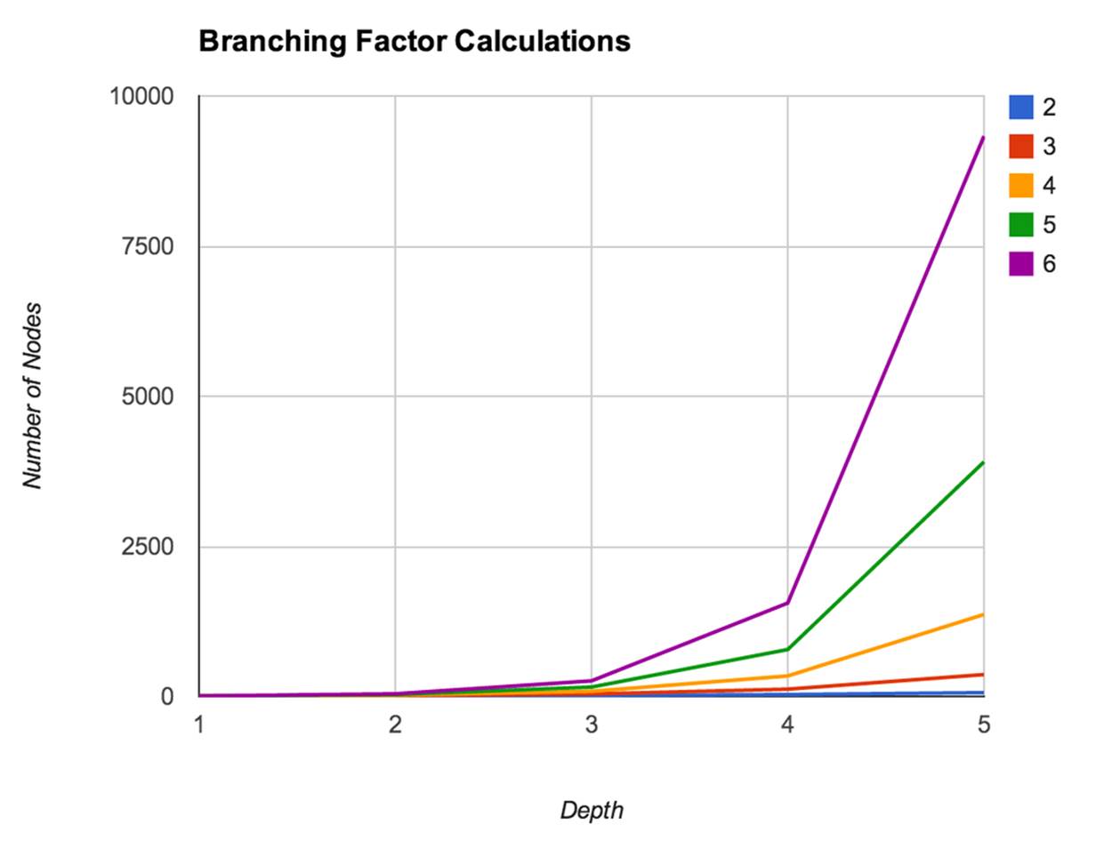
Figure 5-2. The growth in the number of nodes as the depth of a breadth-first search increases
While the previous comments pertain primarily to the theoretical bounds of the algorithm, one final consideration worth noting is the practical performance of the algorithm for a data set of a fixed size. Mild profiling of a breadth-first implementation that fetches web pages would likely reveal that the code is primarily I/O bound from the standpoint that the vast majority of time is spent waiting for a library call to return content to be processed. In situations in which you are I/O bound, a thread pool is a common technique for increasing performance.
Discovering Semantics by Decoding Syntax
You may recall from the previous chapter that perhaps the most fundamental weaknesses of TF-IDF and cosine similarity are that these models inherently don’t leverage a deep semantic understanding of the data and throw away a lot of critical context. Quite the contrary, the examples in that chapter took advantage of very basic syntax that separated tokens by whitespace to break an otherwise opaque document into a bag of words and used frequency and simple statistical similarity metrics to determine which tokens were likely to be important in the data. Although you can do some really amazing things with these techniques, they don’t really give you any notion of what any given token means in the context in which it appears in the document. Look no further than a sentence containing a homograph[18] such as fish, bear, or even google as a case in point; either one could be a noun or a verb.
NLP is inherently complex and difficult to do even reasonably well, and completely nailing it for a large set of commonly spoken languages may well be the problem of the century. However, despite what many believe, it’s far from being a solved problem, and it is already the case that we are starting to see a rising interest in a “deeper understanding” of the Web with initiatives such as Google’s Knowledge Graph, which is being promoted as “the future of search.” After all, a complete mastery of NLP is essentially a plausible strategy for acing the Turing Test, and to the most careful observer, a computer program that achieves this level of “understanding” demonstrates an uncanny amount of human-like intelligence even if it is through a brain that’s mathematically modeled in software as opposed to a biological one.
Whereas structured or semistructured sources are essentially collections of records with some presupposed meaning given to each field that can immediately be analyzed, there are more subtle considerations to be handled with human language data for even the seemingly simplest of tasks. For example, let’s suppose you’re given a document and asked to count the number of sentences in it. It’s a trivial task if you’re a human and have just a basic understanding of English grammar, but it’s another story entirely for a machine, which will require a complex and detailed set of instructions to complete the same task.
The encouraging news is that machines can detect the ends of sentences on relatively well-formed data quickly and with nearly perfect accuracy. Even if you’ve accurately detected all of the sentences, though, there’s still a lot that you probably don’t know about the ways that words or phrases are used in those sentences. Look no further than sarcasm or other forms of ironic language as cases in point. Even with perfect information about the structure of a sentence, you often still need additional context outside the sentence to properly interpret it.
Thus, as an overly broad generalization, we can say that NLP is fundamentally about taking an opaque document that consists of an ordered collection of symbols adhering to proper syntax and a reasonably well-defined grammar, and deducing the semantics associated with those symbols.
Let’s get back to the task of detecting sentences, the first step in most NLP pipelines, to illustrate some of the complexity involved in NLP. It’s deceptively easy to overestimate the utility of simple rule-based heuristics, and it’s important to work through an exercise so that you realize what some of the key issues are and don’t waste time trying to reinvent the wheel.
Your first attempt at solving the sentence detection problem might be to just count the periods, question marks, and exclamation points in the sentence. That’s the most obvious heuristic for starting out, but it’s quite crude and has the potential for producing an extremely high margin of error. Consider the following (relatively unambiguous) accusation:
Mr. Green killed Colonel Mustard in the study with the candlestick. Mr. Green is not a very nice fellow.
Simply tokenizing the sentence by splitting on punctuation (specifically, periods) would produce the following result:
>>> txt="Mr. Green killed Colonel Mustard in the study with the \
... candlestick.Mr.Green is not averynicefellow."
>>> txt.split(".")
['Mr', 'Green killed Colonel Mustard in the study with the candlestick',
'Mr', 'Green is not a very nice fellow', '']
It should be immediately obvious that performing sentence detection by blindly breaking on periods without incorporating some notion of context or higher-level information is insufficient. In this case, the problem is the use of “Mr.,” a valid abbreviation that’s commonly used in the English language. Although we already know from the previous chapter that n-gram analysis of this sample would likely tell us that “Mr. Green” is really one compound token called a collocation or chunk, if we had a larger amount of text to analyze, it’s not hard to imagine other edge cases that would be difficult to detect based on the appearance of collocations. Thinking ahead a bit, it’s also worth pointing out that finding the key topics in a sentence isn’t easy to accomplish with trivial logic either. As an intelligent human, you can easily discern that the key topics in our sample might be “Mr. Green,” “Colonel Mustard,” “the study,” and “the candlestick,” but training a machine to tell you the same things without human intervention is a complex task.
NOTE
Take a moment to think about how you might write a computer program to solve the problem before continuing in order to get the most out of the remainder of this discussion.
A few obvious possibilities are probably occurring to you, such as doing some “Title Case” detection with a regular expression, constructing a list of common abbreviations to parse out the proper noun phrases, and applying some variation of that logic to the problem of finding end-of-sentence (EOS) boundaries to prevent yourself from getting into trouble on that front. OK, sure. Those things will work for some examples, but what’s the margin of error going to be like for arbitrary English text? How forgiving is your algorithm for poorly formed English text; highly abbreviated information such as text messages or tweets; or (gasp) other romantic languages, such as Spanish, French, or Italian? There are no simple answers here, and that’s why text analytics is such an important topic in an age where the amount of digitally available human language data is literally increasing every second.
Natural Language Processing Illustrated Step-by-Step
Let’s prepare to step through a series of examples that illustrate NLP with NLTK. The NLP pipeline we’ll examine involves the following steps:
1. EOS detection
2. Tokenization
3. Part-of-speech tagging
4. Chunking
5. Extraction
We’ll continue to use the following sample text from the previous chapter for the purposes of illustration: “Mr. Green killed Colonel Mustard in the study with the candlestick. Mr. Green is not a very nice fellow.” Remember that even though you have already read the text and understand its underlying grammatical structure, it’s merely an opaque string value to a machine at this point. Let’s look at the steps we need to work through in more detail.
NOTE
The following NLP pipeline is presented as though it is unfolding in a Python interpreter session for clarity and ease of illustration in the input and expected output of each step. However, each step of the pipeline is preloaded into this chapter’s IPython Notebook so that you can follow along per the norm with all other examples.
The five steps are:
EOS detection
This step breaks a text into a collection of meaningful sentences. Since sentences generally represent logical units of thought, they tend to have a predictable syntax that lends itself well to further analysis. Most NLP pipelines you’ll see begin with this step because tokenization (the next step) operates on individual sentences. Breaking the text into paragraphs or sections might add value for certain types of analysis, but it is unlikely to aid in the overall task of EOS detection. In the interpreter, you’d parse out a sentence with NLTK like so:
>>> import nltk
>>> txt = "Mr. Green killed Colonel Mustard in the study with the \
... candlestick. Mr. Green is not a very nice fellow."
>>> txt = "Mr. Green killed Colonel Mustard in the study with the \
... candlestick.Mr. Green is not a very nice fellow."
>>> sentences = nltk.tokenize.sent_tokenize(txt)
>>> sentences
['Mr. Green killed Colonel Mustard in the study with the candlestick.',
'Mr. Green is not a very nice fellow.']
We’ll talk a little bit more about what is happening under the hood with sent_tokenize in the next section. For now, we’ll accept at face value that proper sentence detection has occurred for arbitrary text—a clear improvement over breaking on characters that are likely to be punctuation marks.
Tokenization
This step operates on individual sentences, splitting them into tokens. Following along in the example interpreter session, you’d do the following:
>>> tokens= [nltk.tokenize.word_tokenize(s) fors in sentences]
>>> tokens
[['Mr.', 'Green', 'killed', 'Colonel', 'Mustard', 'in', 'the', 'study',
'with', 'the', 'candlestick', '.'],
['Mr.', 'Green', 'is', 'not', 'a', 'very', 'nice', 'fellow', '.']]
Note that for this simple example, tokenization appeared to do the same thing as splitting on whitespace, with the exception that it tokenized out EOS markers (the periods) correctly. As we’ll see in a later section, though, it can do a bit more if we give it the opportunity, and we already know that distinguishing between whether a period is an EOS marker or part of an abbreviation isn’t always trivial. As an anecdotal note, some written languages, such as ones that use pictograms as opposed to letters, don’t necessarily even require whitespace to separate the tokens in sentences and require the reader (or machine) to distinguish the boundaries.
POS tagging
This step assigns part-of-speech (POS) information to each token. In the example interpreter session, you’d run the tokens through one more step to have them decorated with tags:
>>> pos_tagged_tokens= [nltk.pos_tag(t) fort in tokens]
>>> pos_tagged_tokens
[[('Mr.', 'NNP'), ('Green', 'NNP'), ('killed', 'VBD'), ('Colonel', 'NNP'),
('Mustard', 'NNP'), ('in', 'IN'), ('the', 'DT'), ('study', 'NN'),
('with', 'IN'), ('the', 'DT'), ('candlestick', 'NN'), ('.', '.')],
[('Mr.', 'NNP'), ('Green', 'NNP'), ('is', 'VBZ'), ('not', 'RB'),
('a', 'DT'), ('very', 'RB'), ('nice', 'JJ'), ('fellow', 'JJ'),
('.', '.')]]
You may not intuitively understand all of these tags, but they do represent POS information. For example, 'NNP' indicates that the token is a noun that is part of a noun phrase, 'VBD' indicates a verb that’s in simple past tense, and 'JJ' indicates an adjective. The Penn Treebank Projectprovides a full summary of the POS tags that could be returned. With POS tagging completed, it should be getting pretty apparent just how powerful analysis can become. For example, by using the POS tags, we’ll be able to chunk together nouns as part of noun phrases and then try to reason about what types of entities they might be (e.g., people, places, or organizations). If you never thought that you’d need to apply those exercises from elementary school regarding parts of speech, think again: it’s essential to a proper application of natural language processing.
Chunking
This step involves analyzing each tagged token within a sentence and assembling compound tokens that express logical concepts—quite a different approach than statistically analyzing collocations. It is possible to define a custom grammar through NLTK’s chunk.RegexpParser, but that’s beyond the scope of this chapter; see Chapter 9 (“Building Feature Based Grammars”) of Natural Language Processing with Python (O’Reilly) for full details. Besides, NLTK exposes a function that combines chunking with named entity extraction, which is the next step.
Extraction
This step involves analyzing each chunk and further tagging the chunks as named entities, such as people, organizations, locations, etc. The continuing saga of NLP in the interpreter demonstrates:
>>> ne_chunks=nltk.batch_ne_chunk(pos_tagged_tokens)
>>> printne_chunks
[Tree('S', [Tree('PERSON', [('Mr.', 'NNP')]),
Tree('PERSON', [('Green', 'NNP')]), ('killed', 'VBD'),
Tree('ORGANIZATION', [('Colonel', 'NNP'), ('Mustard', 'NNP')]),
('in', 'IN'), ('the', 'DT'), ('study', 'NN'), ('with', 'IN'),
('the', 'DT'), ('candlestick', 'NN'), ('.', '.')]),
Tree('S', [Tree('PERSON', [('Mr.', 'NNP')]),
Tree('ORGANIZATION',
[('Green', 'NNP')]), ('is', 'VBZ'), ('not', 'RB'),
('a', 'DT'), ('very', 'RB'), ('nice', 'JJ'),
('fellow', 'JJ'), ('.', '.')])]
>>> printne_chunks[0].pprint() # You can pretty-print each chunk in the tree
(S
(PERSONMr./NNP)
(PERSONGreen/NNP)
killed/VBD
(ORGANIZATIONColonel/NNPMustard/NNP)
in/IN
the/DT
study/NN
with/IN
the/DT
candlestick/NN
./.)
Don’t get too wrapped up in trying to decipher exactly what the tree output means just yet. In short, it has chunked together some tokens and attempted to classify them as being certain types of entities. (You may be able to discern that it has identified “Mr. Green” as a person, but unfortunately categorized “Colonel Mustard” as an organization.) Figure 5-3 illustrates output in IPython Notebook.
As worthwhile as it would be to continue exploring natural language with NLTK, that level of engagement isn’t really our purpose here. The background in this section is provided to motivate an appreciation for the difficulty of the task and to encourage you to review the NLTK book or one of the many other plentiful resources available online if you’d like to pursue the topic further.
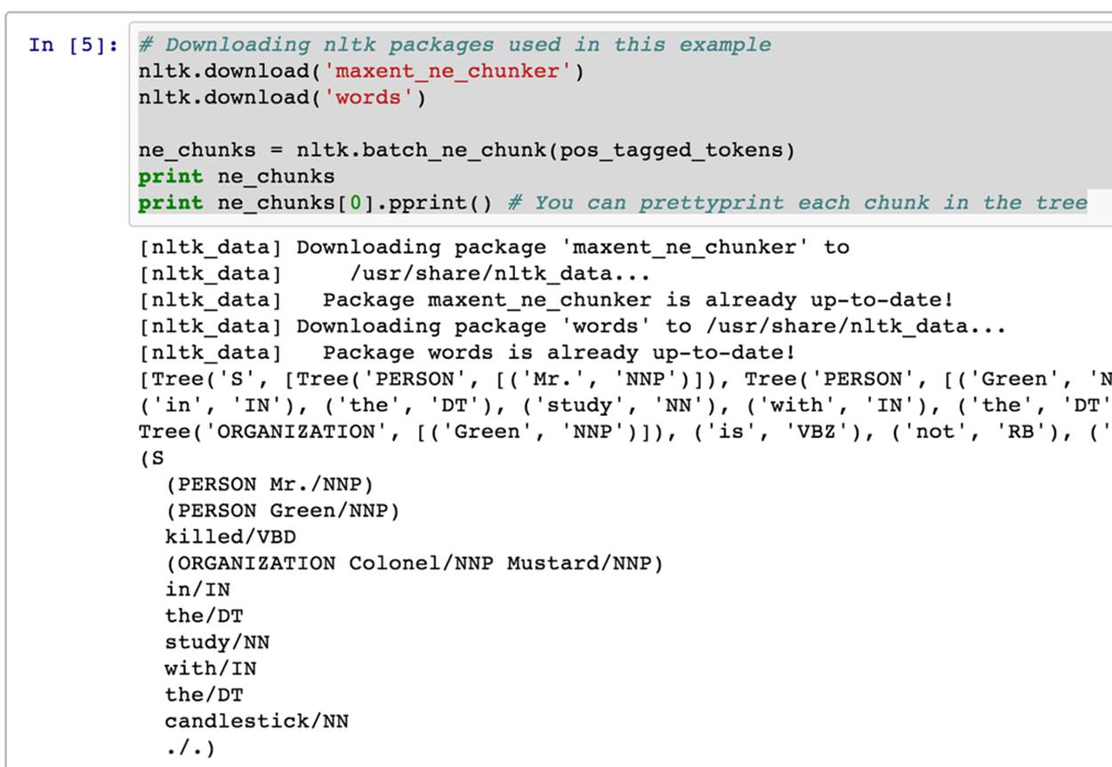
Figure 5-3. NLTK can interface with drawing toolkits so that you can inspect the chunked output in a more intuitive visual form than the raw text output you see in the interpreter
Given that it’s possible to customize certain aspects of NLTK, the remainder of this chapter assumes you’ll be using NLTK “as is” unless otherwise noted.
With that brief introduction to NLP concluded, let’s get to work mining some blog data.
Sentence Detection in Human Language Data
Given that sentence detection is probably the first task you’ll want to ponder when building an NLP stack, it makes sense to start there. Even if you never complete the remaining tasks in the pipeline, it turns out that EOS detection alone yields some powerful possibilities, such as document summarization, which we’ll be considering as a follow-up exercise in the next section. But first, we’ll need to fetch some clean human language data. Let’s use the tried-and-true feedparser package, along with some utilities introduced in the previous chapter that are based on nltk andBeautifulSoup, to clean up HTML formatting that may appear in the content to fetch some posts from the O’Reilly Radar blog. The listing in Example 5-4 fetches a few posts and saves them to a local file as JSON.
Example 5-4. Harvesting blog data by parsing feeds
importos
importsys
importjson
importfeedparser
fromBeautifulSoupimport BeautifulStoneSoup
fromnltkimport clean_html
FEED_URL = 'http://feeds.feedburner.com/oreilly/radar/atom'
def cleanHtml(html):
return BeautifulStoneSoup(clean_html(html),
convertEntities=BeautifulStoneSoup.HTML_ENTITIES).contents[0]
fp = feedparser.parse(FEED_URL)
print "Fetched %s entries from '%s'" % (len(fp.entries[0].title), fp.feed.title)
blog_posts = []
for e infp.entries:
blog_posts.append({'title': e.title, 'content'
: cleanHtml(e.content[0].value), 'link': e.links[0].href})
out_file = os.path.join('resources', 'ch05-webpages', 'feed.json')
f = open(out_file, 'w')
f.write(json.dumps(blog_posts, indent=1))
f.close()
print 'Wrote output file to %s' % (f.name, )
Obtaining human language data from a reputable source affords us the luxury of assuming good English grammar; hopefully this also means that one of NLTK’s out-of-the-box sentence detectors will work reasonably well. There’s no better way to find out than hacking some code to see what happens, so go ahead and review the code listing in Example 5-5. It introduces the sent_tokenize and word_tokenize methods, which are aliases for NLTK’s currently recommended sentence detector and word tokenizer. A brief discussion of the listing is provided afterward.
Example 5-5. Using NLTK’s NLP tools to process human language in blog data
importjson
importnltk
# Download nltk packages used in this example
nltk.download('stopwords')
BLOG_DATA = "resources/ch05-webpages/feed.json"
blog_data = json.loads(open(BLOG_DATA).read())
# Customize your list of stopwords as needed. Here, we add common
# punctuation and contraction artifacts.
stop_words = nltk.corpus.stopwords.words('english') + [
'.',
',',
'--',
'\'s',
'?',
')',
'(',
':',
'\'',
'\'re',
'"',
'-',
'}',
'{',
u'—',
]
for post inblog_data:
sentences = nltk.tokenize.sent_tokenize(post['content'])
words = [w.lower() for sentence insentences for w in
nltk.tokenize.word_tokenize(sentence)]
fdist = nltk.FreqDist(words)
# Basic stats
num_words = sum([i[1] for i infdist.items()])
num_unique_words = len(fdist.keys())
# Hapaxes are words that appear only once
num_hapaxes = len(fdist.hapaxes())
top_10_words_sans_stop_words = [w for w infdist.items() if w[0]
notinstop_words][:10]
print post['title']
print '\tNum Sentences:'.ljust(25), len(sentences)
print '\tNum Words:'.ljust(25), num_words
print '\tNum Unique Words:'.ljust(25), num_unique_words
print '\tNum Hapaxes:'.ljust(25), num_hapaxes
print '\tTop 10 Most Frequent Words (sans stop words):\n\t\t', \
'\n\t\t'.join(['%s (%s)'
% (w[0], w[1]) for w intop_10_words_sans_stop_words])
The first things you’re probably wondering about are the sent_tokenize and word_tokenize calls. NLTK provides several options for tokenization, but it provides “recommendations” as to the best available via these aliases. At the time of this writing (you can double-check this withpydoc or a command like nltk.tokenize.sent_tokenize? in IPython or IPython Notebook at any time), the sentence detector is the PunktSentenceTokenizer and the word tokenizer is the TreebankWordTokenizer. Let’s take a brief look at each of these.
Internally, the PunktSentenceTokenizer relies heavily on being able to detect abbreviations as part of collocation patterns, and it uses some regular expressions to try to intelligently parse sentences by taking into account common patterns of punctuation usage. A full explanation of the innards of the PunktSentenceTokenizer’s logic is outside the scope of this book, but Tibor Kiss and Jan Strunk’s original paper “Unsupervised Multilingual Sentence Boundary Detection” discusses its approach in a highly readable way, and you should take some time to review it.
As we’ll see in a bit, it is possible to instantiate the PunktSentenceTokenizer with sample text that it trains on to try to improve its accuracy. The type of underlying algorithm that’s used is an unsupervised learning algorithm; it does not require you to explicitly mark up the sample training data in any way. Instead, the algorithm inspects certain features that appear in the text itself, such as the use of capitalization and the co-occurrences of tokens, to derive suitable parameters for breaking the text into sentences.
While NLTK’s WhitespaceTokenizer, which creates tokens by breaking a piece of text on whitespace, would have been the simplest word tokenizer to introduce, you’re already familiar with some of the shortcomings of blindly breaking on whitespace. Instead, NLTK currently recommends the TreebankWordTokenizer, a word tokenizer that operates on sentences and uses the same conventions as the Penn Treebank Project.[19] The one thing that may catch you off guard is that the TreebankWordTokenizer’s tokenization does some less-than-obvious things, such as separately tagging components in contractions and nouns having possessive forms. For example, the parsing for the sentence “I’m hungry” would yield separate components for “I” and “’m,” maintaining a distinction between the subject and verb for the two words conjoined in the contraction “I’m.” As you might imagine, finely grained access to this kind of grammatical information can be quite valuable when it’s time to do advanced analysis that scrutinizes relationships between subjects and verbs in sentences.
Given a sentence tokenizer and a word tokenizer, we can first parse the text into sentences and then parse each sentence into tokens. While this approach is fairly intuitive, its Achilles’ heel is that errors produced by the sentence detector propagate forward and can potentially bound the upper limit of the quality that the rest of the NLP stack can produce. For example, if the sentence tokenizer mistakenly breaks a sentence on the period after “Mr.” that appears in a section of text such as “Mr. Green killed Colonel Mustard in the study with the candlestick,” it may not be possible to extract the entity “Mr. Green” from the text unless specialized repair logic is in place. Again, it all depends on the sophistication of the full NLP stack and how it accounts for error propagation.
The out-of-the-box PunktSentenceTokenizer is trained on the Penn Treebank corpus and performs quite well. The end goal of the parsing is to instantiate an nltk.FreqDist object (which is like a slightly more sophisticated collections.Counter), which expects a list of tokens. The remainder of the code in Example 5-5 is a straightforward usage of a few of the commonly used NLTK APIs.
NOTE
If you have a lot of trouble with advanced word tokenizers such as NLTK’s TreebankWordTokenizer or PunktWordTokenizer, it’s fine to default to the WhitespaceTokenizer until you decide whether it’s worth the investment to use a more advanced tokenizer. In fact, using a more straightforward tokenizer can often be advantageous. For example, using an advanced tokenizer on data that frequently inlines URLs might be a bad idea.
The aim of this section was to familiarize you with the first step involved in building an NLP pipeline. Along the way, we developed a few metrics that make a feeble attempt at characterizing some blog data. Our pipeline doesn’t involve part-of-speech tagging or chunking (yet), but it should give you a basic understanding of some concepts and get you thinking about some of the subtler issues involved. While it’s true that we could have simply split on whitespace, counted terms, tallied the results, and still gained a lot of information from the data, it won’t be long before you’ll be glad that you took these initial steps toward a deeper understanding of the data. To illustrate one possible application for what you’ve just learned, in the next section we’ll look at a simple document summarization algorithm that relies on little more than sentence segmentation and frequencyanalysis.
Document Summarization
Being able to perform reasonably good sentence detection as part of an NLP approach to mining unstructured data can enable some pretty powerful text-mining capabilities, such as crude but very reasonable attempts at document summarization. There are numerous possibilities and approaches, but one of the simplest to get started with dates all the way back to the April 1958 issue of IBM Journal. In the seminal article entitled “The Automatic Creation of Literature Abstracts,” H.P. Luhn describes a technique that essentially boils down to filtering out sentences containing frequently occurring words that appear near one another.
The original paper is easy to understand and rather interesting; Luhn actually describes how he prepared punch cards in order to run various tests with different parameters! It’s amazing to think that what we can implement in a few dozen lines of Python on a cheap piece of commodity hardware, he probably labored over for hours and hours to program into a gargantuan mainframe. Example 5-6 provides a basic implementation of Luhn’s algorithm for document summarization. A brief analysis of the algorithm appears in the next section. Before skipping ahead to that discussion, first take a moment to trace through the code to learn more about how it works.
NOTE
Example 5-6 uses the numpy package (a collection of highly optimized numeric operations), which should have been installed alongside nltk. If for some reason you are not using the virtual machine and need to install it, just use pip install numpy.
Example 5-6. A document summarization algorithm based principally upon sentence detection and frequency analysis within sentences
importjson
importnltk
importnumpy
BLOG_DATA = "resources/ch05-webpages/feed.json"
N = 100 # Number of words to consider
CLUSTER_THRESHOLD = 5 # Distance between words to consider
TOP_SENTENCES = 5 # Number of sentences to return for a "top n" summary
# Approach taken from "The Automatic Creation of Literature Abstracts" by H.P. Luhn
def _score_sentences(sentences, important_words):
scores = []
sentence_idx = -1
for s in [nltk.tokenize.word_tokenize(s) for s insentences]:
sentence_idx += 1
word_idx = []
# For each word in the word list...
for w inimportant_words:
try:
# Compute an index for where any important words occur in the sentence.
word_idx.append(s.index(w))
exceptValueError, e: # w not in this particular sentence
pass
word_idx.sort()
# It is possible that some sentences may not contain any important words at all.
if len(word_idx)== 0: continue
# Using the word index, compute clusters by using a max distance threshold
# for any two consecutive words.
clusters = []
cluster = [word_idx[0]]
i = 1
while i < len(word_idx):
if word_idx[i] - word_idx[i - 1] < CLUSTER_THRESHOLD:
cluster.append(word_idx[i])
else:
clusters.append(cluster[:])
cluster = [word_idx[i]]
i += 1
clusters.append(cluster)
# Score each cluster. The max score for any given cluster is the score
# for the sentence.
max_cluster_score = 0
for c inclusters:
significant_words_in_cluster = len(c)
total_words_in_cluster = c[-1] - c[0] + 1
score = 1.0 * significant_words_in_cluster \
* significant_words_in_cluster / total_words_in_cluster
if score > max_cluster_score:
max_cluster_score = score
scores.append((sentence_idx, score))
return scores
def summarize(txt):
sentences = [s for s innltk.tokenize.sent_tokenize(txt)]
normalized_sentences = [s.lower() for s insentences]
words = [w.lower() for sentence innormalized_sentences for w in
nltk.tokenize.word_tokenize(sentence)]
fdist = nltk.FreqDist(words)
top_n_words = [w[0] for w infdist.items()
if w[0] notinnltk.corpus.stopwords.words('english')][:N]
scored_sentences = _score_sentences(normalized_sentences, top_n_words)
# Summarization Approach 1:
# Filter out nonsignificant sentences by using the average score plus a
# fraction of the std dev as a filter
avg = numpy.mean([s[1] for s inscored_sentences])
std = numpy.std([s[1] for s inscored_sentences])
mean_scored = [(sent_idx, score) for (sent_idx, score) inscored_sentences
if score > avg + 0.5 * std]
# Summarization Approach 2:
# Another approach would be to return only the top N ranked sentences
top_n_scored = sorted(scored_sentences, key=lambda s: s[1])[-TOP_SENTENCES:]
top_n_scored = sorted(top_n_scored, key=lambda s: s[0])
# Decorate the post object with summaries
return dict(top_n_summary=[sentences[idx] for (idx, score) intop_n_scored],
mean_scored_summary=[sentences[idx] for (idx, score) inmean_scored])
blog_data = json.loads(open(BLOG_DATA).read())
for post inblog_data:
post.update(summarize(post['content']))
print post['title']
print '=' * len(post['title'])
print 'Top N Summary'
print '-------------'
print ' '.join(post['top_n_summary'])
print 'Mean Scored Summary'
print '-------------------'
print ' '.join(post['mean_scored_summary'])
As example input/output, we’ll use Tim O’Reilly’s Radar post, “The Louvre of the Industrial Age”. It’s around 460 words long and is reprinted here so that you can compare the sample output from the two summarization attempts in the listing:
This morning I had the chance to get a tour of The Henry Ford Museum in Dearborn, MI, along with Dale Dougherty, creator of Make: and Makerfaire, and Marc Greuther, the chief curator of the museum. I had expected a museum dedicated to the auto industry, but it’s so much more than that. As I wrote in my first stunned tweet, “it’s the Louvre of the Industrial Age.”
When we first entered, Marc took us to what he said may be his favorite artifact in the museum, a block of concrete that contains Luther Burbank’s shovel, and Thomas Edison’s signature and footprints. Luther Burbank was, of course, the great agricultural inventor who created such treasures as the nectarine and the Santa Rosa plum. Ford was a farm boy who became an industrialist; Thomas Edison was his friend and mentor. The museum, opened in 1929, was Ford’s personal homage to the transformation of the world that he was so much a part of. This museum chronicles that transformation.
The machines are astonishing—steam engines and coal-fired electric generators as big as houses, the first lathes capable of making other precision lathes (the makerbot of the 19th century), a ribbon glass machine that is one of five that in the 1970s made virtually all of the incandescent lightbulbs in the world, combine harvesters, railroad locomotives, cars, airplanes, even motels, gas stations, an early McDonalds’ restaurant and other epiphenomena of the automobile era.
Under Marc’s eye, we also saw the transformation of the machines from purely functional objects to things of beauty. We saw the advances in engineering—the materials, the workmanship, the design, over a hundred years of innovation. Visiting The Henry Ford, as they call it, is a truly humbling experience. I would never in a hundred years have thought of making a visit to Detroit just to visit this museum, but knowing what I know now, I will tell you confidently that it is as worth your while as a visit to Paris just to see the Louvre, to Rome for the Vatican Museum, to Florence for the Uffizi Gallery, to St. Petersburg for the Hermitage, or to Berlin for the Pergamon Museum. This is truly one of the world’s great museums, and the world that it chronicles is our own.
I am truly humbled that the Museum has partnered with us to hold Makerfaire Detroit on their grounds. If you are anywhere in reach of Detroit this weekend, I heartily recommend that you plan to spend both days there. You can easily spend a day at Makerfaire, and you could easily spend a day at The Henry Ford. P.S. Here are some of my photos from my visit. (More to come soon. Can’t upload many as I’m currently on a plane.)
Filtering sentences using an average score and standard deviation yields a summary of around 170 words:
This morning I had the chance to get a tour of The Henry Ford Museum in Dearborn, MI, along with Dale Dougherty, creator of Make: and Makerfaire, and Marc Greuther, the chief curator of the museum. I had expected a museum dedicated to the auto industry, but it’s so much more than that. As I wrote in my first stunned tweet, “it’s the Louvre of the Industrial Age. This museum chronicles that transformation. The machines are astonishing - steam engines and coal fired electric generators as big as houses, the first lathes capable of making other precision lathes (the makerbot of the 19th century), a ribbon glass machine that is one of five that in the 1970s made virtually all of the incandescent lightbulbs in the world, combine harvesters, railroad locomotives, cars, airplanes, even motels, gas stations, an early McDonalds’ restaurant and other epiphenomena of the automobile era. You can easily spend a day at Makerfaire, and you could easily spend a day at The Henry Ford.
An alternative summarization approach, which considers only the top N sentences (where N = 5 in this case), produces a slightly more abridged result of around 90 words. It’s even more succinct, but arguably still a pretty informative distillation:
This morning I had the chance to get a tour of The Henry Ford Museum in Dearborn, MI, along with Dale Dougherty, creator of Make: and Makerfaire, and Marc Greuther, the chief curator of the museum. I had expected a museum dedicated to the auto industry, but it’s so much more than that. As I wrote in my first stunned tweet, “it’s the Louvre of the Industrial Age. This museum chronicles that transformation. You can easily spend a day at Makerfaire, and you could easily spend a day at The Henry Ford.
As in any other situation involving analysis, there’s a lot of insight to be gained from visually inspecting the summarizations in relation to the full text.
Outputting a simple markup format that can be opened by virtually any web browser is as simple as adjusting the final portion of the script that performs the output to do some string substitution. Example 5-7 illustrates one possibility for visualizing the output of document summarization by presenting the full text of the article with the sentences that are included as part of the summary in bold so that it’s easy to see what was included in the summary and what wasn’t. The script saves a collection of HTML files to disk that you can view within your IPython Notebook session or open in a browser without the need for a web server.
Example 5-7. Visualizing document summarization results with HTML output
importos
importjson
importnltk
importnumpy
fromIPython.displayimport IFrame
fromIPython.core.displayimport display
BLOG_DATA = "resources/ch05-webpages/feed.json"
HTML_TEMPLATE = """<html>
<head>
<title>%s</title>
<meta http-equiv="Content-Type" content="text/html; charset=UTF-8"/>
</head>
<body>%s</body>
</html>"""
blog_data = json.loads(open(BLOG_DATA).read())
for post inblog_data:
# Uses previously defined summarize function.
post.update(summarize(post['content']))
# You could also store a version of the full post with key sentences marked up
# for analysis with simple string replacement...
for summary_type in ['top_n_summary', 'mean_scored_summary']:
post[summary_type + '_marked_up'] = '<p>%s</p>' % (post['content'], )
for s inpost[summary_type]:
post[summary_type + '_marked_up'] = \
post[summary_type + '_marked_up'].replace(s, '<strong>%s</strong>' % (s, ))
filename = post['title'].replace("?", "") + '.summary.' + summary_type + '.html'
f = open(os.path.join('resources', 'ch05-webpages', filename), 'w')
html = HTML_TEMPLATE % (post['title'] + \
' Summary', post[summary_type + '_marked_up'],)
f.write(html.encode('utf-8'))
f.close()
print "Data written to", f.name
# Display any of these files with an inline frame. This displays the
# last file processed by using the last value of f.name...
print "Displaying %s:" % f.name
display(IFrame('files/%s' % f.name, '100%', '600px'))
The resulting output is the full text of the document with sentences composing the summary highlighted in bold, as displayed in Figure 5-4. As you explore alternative techniques for summarization, a quick glance between browser tabs can give you an intuitive feel for the similarity between the summarization techniques. The primary difference illustrated here is a fairly long (and descriptive) sentence near the middle of the document, beginning with the words “The machines are astonishing.”
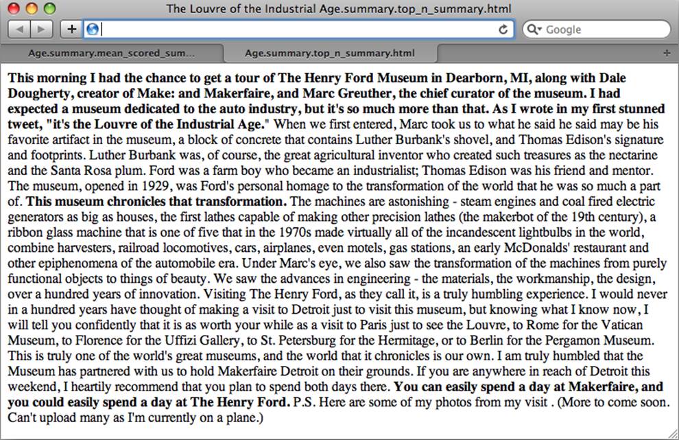
Figure 5-4. A visualization of the text from an O’Reilly Radar blog post with the most important sentences as determined by a summarization algorithm conveyed in bold
The next section presents a brief discussion of Luhn’s document summarization approach.
Analysis of Luhn’s summarization algorithm
NOTE
This section provides an analysis of Luhn’s summarization algorithm. It aims to broaden your understanding of techniques in processing human language data but is certainly not a requirement for mining the social web. If you find yourself getting lost in the details, feel free to skip this section and return to it at a later time.
The basic premise behind Luhn’s algorithm is that the important sentences in a document will be the ones that contain frequently occurring words. However, there are a few details worth pointing out. First, not all frequently occurring words are important; generally speaking, stopwords are filler and are hardly ever of interest for analysis. Keep in mind that although we do filter out common stopwords in the sample implementation, it may be possible to create a custom list of stopwords for any given blog or domain with additional a priori knowledge, which might further bolster the strength of this algorithm or any other algorithm that assumes stopwords have been filtered. For example, a blog written exclusively about baseball might so commonly use the word baseball that you should consider adding it to a stopword list, even though it’s not a general-purpose stopword. (As a side note, it would be interesting to incorporate TF-IDF into the scoring function for a particular data source as a means of accounting for common words in the parlance of the domain.)
Assuming that a reasonable attempt to eliminate stopwords has been made, the next step in the algorithm is to choose a reasonable value for N and choose the top N words as the basis of analysis. The latent assumption behind this algorithm is that these top N words are sufficiently descriptive to characterize the nature of the document, and that for any two sentences in the document, the sentence that contains more of these words will be considered more descriptive. All that’s left after determining the “important words” in the document is to apply a heuristic to each sentence and filter out some subset of sentences to use as a summarization or abstract of the document. Scoring each sentence takes place in the function score_sentences. This is where most of the action happens in the listing.
In order to score each sentence, the algorithm in score_sentences applies a simple distance threshold to cluster tokens, and scores each cluster according to the following formula:
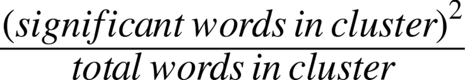
The final score for each sentence is equal to the highest score for any cluster appearing in the sentence. Let’s consider the high-level steps involved in score_sentences for an example sentence to see how this approach works in practice:
Input: Sample sentence
['Mr.', 'Green', 'killed', 'Colonel', 'Mustard', 'in', 'the', 'study', 'with', 'the', 'candlestick', '.']
Input: List of important words
['Mr.', 'Green', 'Colonel', 'Mustard', 'candlestick']
Input/assumption: Cluster threshold (distance)
3
Intermediate computation: Clusters detected
[ ['Mr.', 'Green', 'killed', 'Colonel', 'Mustard'], ['candlestick'] ]
Intermediate computation: Cluster scores
[ 3.2, 1 ] # Computation: [ (4*4)/5, (1*1)/1]
Output: Sentence score
3.2 # max([3.2, 1])
The actual work done in score_sentences is just bookkeeping to detect the clusters in the sentence. A cluster is defined as a sequence of words containing two or more important words, where each important word is within a distance threshold of its nearest neighbor. While Luhn’s paper suggests a value of 4 or 5 for the distance threshold, we used a value of 3 for simplicity in this example; thus, the distance between 'Green' and 'Colonel' was sufficiently bridged, and the first cluster detected consisted of the first five words in the sentence. Had the word study also appeared in the list of important words, the entire sentence (except the final punctuation) would have emerged as a cluster.
Once each sentence has been scored, all that’s left is to determine which sentences to return as a summary. The sample implementation provides two approaches. The first approach uses a statistical threshold to filter out sentences by computing the mean and standard deviation for the scores obtained, while the latter simply returns the top N sentences. Depending on the nature of the data, your mileage will vary, but you should be able to tune the parameters to achieve reasonable results with either. One nice thing about using the top N sentences is that you have a pretty good idea about the maximum length of the summary. Using the mean and standard deviation could potentially return more sentences than you’d prefer, if a lot of sentences contain scores that are relatively close to one another.
Luhn’s algorithm is simple to implement and plays to the usual strength of frequently appearing words being descriptive of the overall document. However, keep in mind that like many of the approaches based on the classic information retrieval concepts we explored in the previous chapter, Luhn’s algorithm itself makes no attempt to understand the data at a deeper semantic level—although it does depend on more than just a “bag of words.” It directly computes summarizations as a function of frequently occurring words, and it isn’t terribly sophisticated in how it scores sentences, but (as was the case with TF-IDF), this just makes it all the more amazing that it can perform as well as it seems to perform on randomly selected blog data.
When you’re weighing the pros and cons of implementing a much more complicated approach, it’s worth reflecting on the effort that would be required to improve upon a reasonable summarization such as that produced by Luhn’s algorithm. Sometimes, a crude heuristic is all you really need to accomplish your goal. At other times, however, you may need something more cutting-edge. The tricky part is computing the cost-benefit analysis of migrating from the crude heuristic to the state-of-the-art solution. Many of us tend to be overly optimistic about the relative effort involved.
Entity-Centric Analysis: A Paradigm Shift
Throughout this chapter, it’s been implied that analytic approaches that exhibit a deeper understanding of the data can be dramatically more powerful than approaches that simply treat each token as an opaque symbol. But what does a “deeper understanding” of the data really mean?
One interpretation is being able to detect the entities in documents and using those entities as the basis of analysis, as opposed to doing document-centric analysis involving keyword searches or interpreting a search input as a particular type of entity and customizing the results accordingly. Although you may not have thought about it in those terms, this is precisely what emerging technologies such as WolframAlpha do at the presentation layer. For example, a search for “tim o’reilly” in WolframAlpha returns results that imply an understanding that the entity being searched for is a person; you don’t just get back a list of documents containing the keywords (see Figure 5-5). Regardless of the internal technique that’s used to accomplish this end, the resulting user experience is dramatically more powerful because the results conform to a format that more closely satisfies the user’s expectations.
Although we can’t ponder all of the various possibilities of entity-centric analysis in the current discussion, it’s well within our reach and quite appropriate to present a means of extracting the entities from a document, which can then be used for various analytic purposes. Assuming the sample flow of an NLP pipeline as presented earlier in this chapter, you could simply extract all the nouns and noun phrases from the document and index them as entities appearing in the documents—the important underlying assumption being that nouns and noun phrases (or some carefully constructed subset thereof) qualify as entities of interest. This is actually a fair assumption to make and a good starting point for entity-centric analysis, as the following sample listing demonstrates. Note that for results annotated according to Penn Treebank conventions, any tag beginning with 'NN' is some form of a noun or noun phrase. A full listing of the Penn Treebank tags is available online.
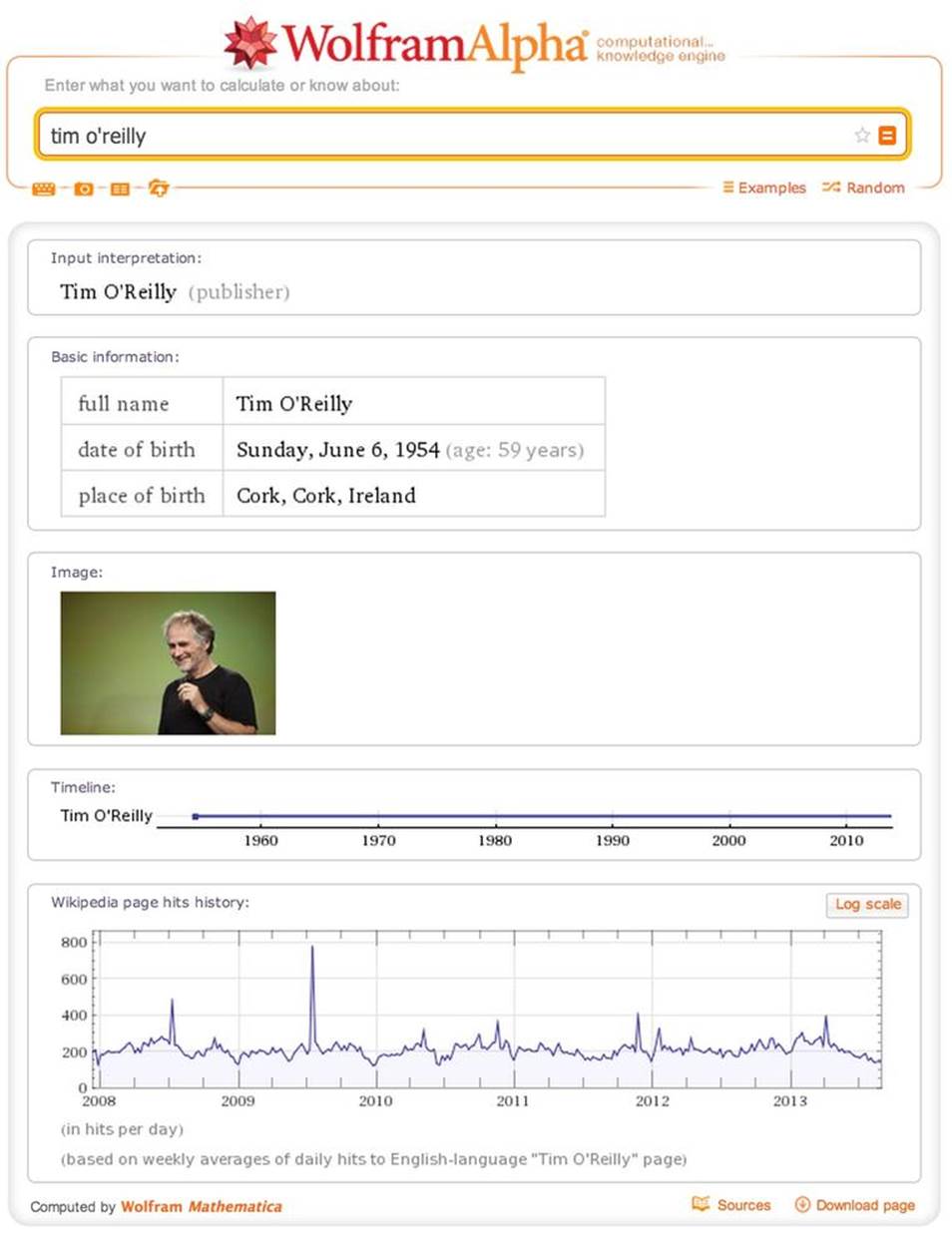
Figure 5-5. Sample results for a “tim o’reilly” query with WolframAlpha
Example 5-8 analyzes the part-of-speech tags that are applied to tokens, and identifies nouns and noun phrases as entities. In data mining parlance, finding the entities in a text is called entity extraction or named entity recognition, depending on the nuances of exactly what you are trying to accomplish.
Example 5-8. Extracting entities from a text with NLTK
importnltk
importjson
BLOG_DATA = "resources/ch05-webpages/feed.json"
blog_data = json.loads(open(BLOG_DATA).read())
for post inblog_data:
sentences = nltk.tokenize.sent_tokenize(post['content'])
tokens = [nltk.tokenize.word_tokenize(s) for s insentences]
pos_tagged_tokens = [nltk.pos_tag(t) for t intokens]
# Flatten the list since we're not using sentence structure
# and sentences are guaranteed to be separated by a special
# POS tuple such as ('.', '.')
pos_tagged_tokens = [token for sent inpos_tagged_tokens for token insent]
all_entity_chunks = []
previous_pos = None
current_entity_chunk = []
for (token, pos) inpos_tagged_tokens:
if pos == previous_pos andpos.startswith('NN'):
current_entity_chunk.append(token)
elif pos.startswith('NN'):
if current_entity_chunk != []:
# Note that current_entity_chunk could be a duplicate when appended,
# so frequency analysis again becomes a consideration
all_entity_chunks.append((' '.join(current_entity_chunk), pos))
current_entity_chunk = [token]
previous_pos = pos
# Store the chunks as an index for the document
# and account for frequency while we're at it...
post['entities'] = {}
for c inall_entity_chunks:
post['entities'][c] = post['entities'].get(c, 0) + 1
# For example, we could display just the title-cased entities
print post['title']
print '-' * len(post['title'])
proper_nouns = []
for (entity, pos) inpost['entities']:
if entity.istitle():
print '\t%s (%s)' % (entity, post['entities'][(entity, pos)])
NOTE
You may recall from the description of “extraction” in Natural Language Processing Illustrated Step-by-Step that NLTK provides an nltk.batch_ne_chunk function that attempts to extract named entities from POS-tagged tokens. You’re welcome to use this capability directly, but you may find that your mileage varies with the out-of-the-box models provided with the NLTK implementation.
Sample output for the listing is presented next and conveys results that are quite meaningful and could be used in a variety of ways. For example, they would make great suggestions for tagging posts by an intelligent blogging platform like a WordPress plugin:
The Louvre of the Industrial Age
--------------------------------
Paris (1)
Henry Ford Museum (1)
Vatican Museum (1)
Museum (1)
Thomas Edison (2)
Hermitage (1)
Uffizi Gallery (1)
Ford (2)
Santa Rosa (1)
Dearborn (1)
Makerfaire (1)
Berlin (1)
Marc (2)
Makerfaire (1)
Rome (1)
Henry Ford (1)
Ca (1)
Louvre (1)
Detroit (2)
St. Petersburg (1)
Florence (1)
Marc Greuther (1)
Makerfaire Detroit (1)
Luther Burbank (2)
Make (1)
Dale Dougherty (1)
Louvre (1)
Statistical artifacts often have different purposes and consumers. A text summary is meant to be read, whereas a list of extracted entities like the preceding one lends itself to being scanned quickly for patterns. For a larger corpus than we’re working with in this example, a tag cloud could be an obvious candidate for visualizing the data.
NOTE
Try reproducing these results by scraping the text from the web page http://oreil.ly/1a1n4SO.
Could we have discovered the same list of terms by more blindly analyzing the lexical characteristics (such as use of capitalization) of the sentence? Perhaps, but keep in mind that this technique can also capture nouns and noun phrases that are not indicated by title case. Case is indeed an important feature of the text that can generally be exploited to great benefit, but there are other intriguing entities in the sample text that are all lowercase (for example, “chief curator,” “locomotives,” and “lightbulbs”).
Although the list of entities certainly doesn’t convey the overall meaning of the text as effectively as the summary we computed earlier, identifying these entities can be extremely valuable for analysis since they have meaning at a semantic level and are not just frequently occurring words. In fact, the frequencies of most of the terms displayed in the sample output are quite low. Nevertheless, they’re important because they have a grounded meaning in the text—namely, they’re people, places, things, or ideas, which are generally the substantive information in the data.
Gisting Human Language Data
It’s not much of a leap at this point to think that it would be another major step forward to take into account the verbs and compute triples of the form subject-verb-object so that you know which entities are interacting with which other entities, and the nature of those interactions. Such triples would lend themselves to visualizing object graphs of documents, which we could potentially skim much faster than we could read the documents themselves. Better yet, imagine taking multiple object graphs derived from a set of documents and merging them to get the gist of the larger corpus. This exact technique is an area of active research and has tremendous applicability for virtually any situation suffering from the information-overload problem. But as will be illustrated, it’s an excruciating problem for the general case and not for the faint of heart.
Assuming a part-of-speech tagger has identified the parts of speech from a sentence and emitted output such as [('Mr.', 'NNP'), ('Green', 'NNP'), ('killed', 'VBD'), ('Colonel', 'NNP'), ('Mustard', 'NNP'), ...], an index storing subject-predicate-object tuples of the form ('Mr. Green', 'killed', 'Colonel Mustard') would be easy to compute. However, the reality of the situation is that you’re unlikely to run across actual POS-tagged data with that level of simplicity—unless you’re planning to mine children’s books (not actually a bad starting point for testing toy ideas). For example, consider the tagging emitted from NLTK for the first sentence from the blog post printed earlier in this chapter as an arbitrary and realistic piece of data you might like to translate into an object graph:
This morning I had the chance to get a tour of The Henry Ford Museum in Dearborn, MI, along with Dale Dougherty, creator of Make: and Makerfaire, and Marc Greuther, the chief curator of the museum.
The simplest possible triple that you might expect to distill from that sentence is ('I', 'get', 'tour'), but even if you got that back, it wouldn’t convey that Dale Dougherty also got the tour, or that Marc Greuther was involved. The POS-tagged data should make it pretty clear that it’s not quite so straightforward to arrive at any of those interpretations, either, because the sentence has a very rich structure:
[(u'This', 'DT'), (u'morning', 'NN'), (u'I', 'PRP'), (u'had', 'VBD'),
(u'the', 'DT'), (u'chance', 'NN'), (u'to', 'TO'), (u'get', 'VB'),
(u'a', 'DT'), (u'tour', 'NN'), (u'of', 'IN'), (u'The', 'DT'),
(u'Henry', 'NNP'), (u'Ford', 'NNP'), (u'Museum', 'NNP'), (u'in', 'IN'),
(u'Dearborn', 'NNP'), (u',', ','), (u'MI', 'NNP'), (u',', ','),
(u'along', 'IN'), (u'with', 'IN'), (u'Dale', 'NNP'), (u'Dougherty', 'NNP'),
(u',', ','), (u'creator', 'NN'), (u'of', 'IN'), (u'Make', 'NNP'), (u':', ':'),
(u'and', 'CC'), (u'Makerfaire', 'NNP'), (u',', ','), (u'and', 'CC'),
(u'Marc', 'NNP'), (u'Greuther', 'NNP'), (u',', ','), (u'the', 'DT'),
(u'chief', 'NN'), (u'curator', 'NN'), (u'of', 'IN'), (u'the', 'DT'),
(u'museum', 'NN'), (u'.', '.')]
It’s doubtful that a high-quality open source NLP toolkit would be capable of emitting meaningful triples in this case, given the complex nature of the predicate “had a chance to get a tour” and that the other actors involved in the tour are listed in a phrase appended to the end of the sentence.
NOTE
If you’d like to pursue strategies for constructing these triples, you should be able to use reasonably accurate POS tagging information to take a good initial stab at it. Advanced tasks in manipulating human language data can be a lot of work, but the results are satisfying and have the potential to be quite disruptive (in a good way).
The good news is that you can actually do a lot of fun things by distilling just the entities from text and using them as the basis of analysis, as demonstrated earlier. You can easily produce triples from text on a per-sentence basis, where the “predicate” of each triple is a notion of a generic relationship signifying that the subject and object “interacted” with each other. Example 5-9 is a refactoring of Example 5-8 that collects entities on a per-sentence basis, which could be quite useful for computing the interactions between entities using a sentence as a context window.
Example 5-9. Discovering interactions between entities
importnltk
importjson
BLOG_DATA = "resources/ch05-webpages/feed.json"
def extract_interactions(txt):
sentences = nltk.tokenize.sent_tokenize(txt)
tokens = [nltk.tokenize.word_tokenize(s) for s insentences]
pos_tagged_tokens = [nltk.pos_tag(t) for t intokens]
entity_interactions = []
for sentence inpos_tagged_tokens:
all_entity_chunks = []
previous_pos = None
current_entity_chunk = []
for (token, pos) insentence:
if pos == previous_pos andpos.startswith('NN'):
current_entity_chunk.append(token)
elif pos.startswith('NN'):
if current_entity_chunk != []:
all_entity_chunks.append((' '.join(current_entity_chunk),
pos))
current_entity_chunk = [token]
previous_pos = pos
if len(all_entity_chunks) > 1:
entity_interactions.append(all_entity_chunks)
else:
entity_interactions.append([])
assert len(entity_interactions) == len(sentences)
return dict(entity_interactions=entity_interactions,
sentences=sentences)
blog_data = json.loads(open(BLOG_DATA).read())
# Display selected interactions on a per-sentence basis
for post inblog_data:
post.update(extract_interactions(post['content']))
print post['title']
print '-' * len(post['title'])
for interactions inpost['entity_interactions']:
print '; '.join([i[0] for i ininteractions])
The following results from this listing highlight something important about the nature of unstructured data analysis: it’s messy!
The Louvre of the Industrial Age
--------------------------------
morning; chance; tour; Henry Ford Museum; Dearborn; MI; Dale Dougherty; creator;
Make; Makerfaire; Marc Greuther; chief curator
tweet; Louvre
"; Marc; artifact; museum; block; contains; Luther Burbank; shovel; Thomas Edison
Luther Burbank; course; inventor; treasures; nectarine; Santa Rosa
Ford; farm boy; industrialist; Thomas Edison; friend
museum; Ford; homage; transformation; world
machines; steam; engines; coal; generators; houses; lathes; precision; lathes;
makerbot; century; ribbon glass machine; incandescent; lightbulbs; world; combine;
harvesters; railroad; locomotives; cars; airplanes; gas; stations; McDonalds;
restaurant; epiphenomena
Marc; eye; transformation; machines; objects; things
advances; engineering; materials; workmanship; design; years
years; visit; Detroit; museum; visit; Paris; Louvre; Rome; Vatican Museum;
Florence; Uffizi Gallery; St. Petersburg; Hermitage; Berlin
world; museums
Museum; Makerfaire Detroit
reach; Detroit; weekend
day; Makerfaire; day
A certain amount of noise in the results is almost inevitable, but realizing results that are highly intelligible and useful—even if they do contain a manageable amount of noise—is a worthy aim. The amount of effort required to achieve pristine results that are nearly noise-free can be immense. In fact, in most situations, this is downright impossible because of the inherent complexity involved in natural language and the limitations of most currently available toolkits, including NLTK. If you are able to make certain assumptions about the domain of the data or have expert knowledge of the nature of the noise, you may be able to devise heuristics that are effective without risking an unacceptable amount of information loss—but it’s a fairly difficult proposition.
Still, the interactions do provide a certain amount of “gist” that’s valuable. For example, how closely would your interpretation of “morning; chance; tour; Henry Ford Museum; Dearborn; MI; Dale Dougherty; creator; Make; Makerfaire; Marc Greuther; chief curator” align with the meaning in the original sentence?
As was the case with our previous adventure in summarization, displaying markup that can be visually skimmed for inspection is also quite handy. A simple modification to Example 5-9 output, as shown in Example 5-10, is all that’s necessary to produce the results shown in Figure 5-6.
Example 5-10. Visualizing interactions between entities with HTML output
importos
importjson
importnltk
fromIPython.displayimport IFrame
fromIPython.core.displayimport display
BLOG_DATA = "resources/ch05-webpages/feed.json"
HTML_TEMPLATE = """<html>
<head>
<title>%s</title>
<meta http-equiv="Content-Type" content="text/html; charset=UTF-8"/>
</head>
<body>%s</body>
</html>"""
blog_data = json.loads(open(BLOG_DATA).read())
for post inblog_data:
post.update(extract_interactions(post['content']))
# Display output as markup with entities presented in bold text
post['markup'] = []
for sentence_idx inrange(len(post['sentences'])):
s = post['sentences'][sentence_idx]
for (term, _) inpost['entity_interactions'][sentence_idx]:
s = s.replace(term, '<strong>%s</strong>' % (term, ))
post['markup'] += [s]
filename = post['title'].replace("?", "") + '.entity_interactions.html'
f = open(os.path.join('resources', 'ch05-webpages', filename), 'w')
html = HTML_TEMPLATE % (post['title'] + ' Interactions',
' '.join(post['markup']),)
f.write(html.encode('utf-8'))
f.close()
print "Data written to", f.name
# Display any of these files with an inline frame. This displays the
# last file processed by using the last value of f.name...
print "Displaying %s:" % f.name
display(IFrame('files/%s' % f.name, '100%', '600px'))
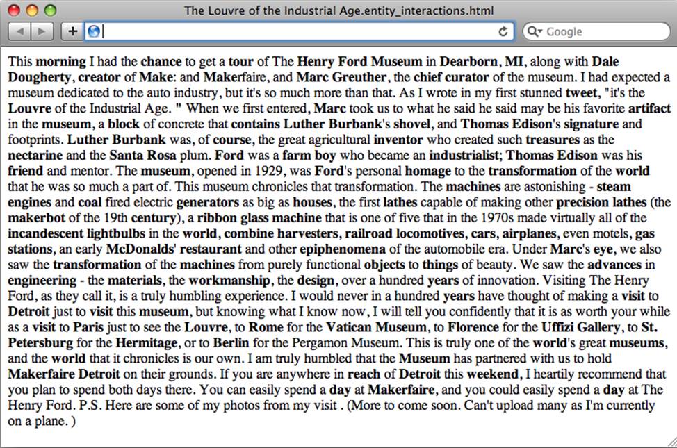
Figure 5-6. Sample HTML output that displays entities identified in the text in bold so that it’s easy to visually skim the content for its key concepts
It could also be fruitful to perform additional analyses to identify the sets of interactions for a larger body of text and to find and visualize co-occurrences in the interactions. The code involving force-directed graphs illustrated in Visualizing directed graphs of mutual friendships would make a good starting template for visualization, but even without knowing the specific nature of the interaction, there’s still a lot of value in just knowing the subject and the object. If you’re feeling ambitious, you should attempt to complete the tuples with the missing verbs.
Quality of Analytics for Processing Human Language Data
When you’ve done even a modest amount of text mining, you’ll eventually want to start quantifying the quality of your analytics. How accurate is your end-of-sentence detector? How accurate is your part-of-speech tagger? For example, if you began customizing the basic algorithm for extracting the entities from unstructured text, how would you know whether your algorithm was getting more or less performant with respect to the quality of the results? While you could manually inspect the results for a small corpus and tune the algorithm until you were satisfied with them, you’d still have a devil of a time determining whether your analytics would perform well on a much larger corpus or a different class of document altogether—hence, the need for a more automated process.
An obvious starting point is to randomly sample some documents and create a “golden set” of entities that you believe are absolutely crucial for a good algorithm to extract from them, and then use this list as the basis of evaluation. Depending on how rigorous you’d like to be, you might even be able to compute the sample error and use a statistical device called a confidence interval to predict the true error with a sufficient degree of confidence for your needs. However, what exactly is the calculation you should be computing based on the results of your extractor and golden set in order to compute accuracy? A very common calculation for measuring accuracy is called the F1 score, which is defined in terms of two concepts called precision and recall[20] as:
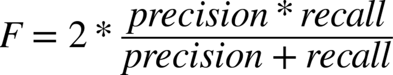
where:
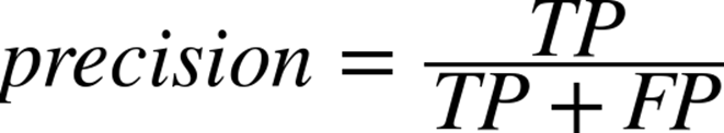
and:
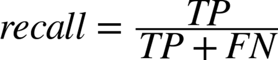
In the current context, precision is a measure of exactness that reflects false positives, and recall is a measure of completeness that reflects true positives. The following list clarifies the meaning of these terms in relation to the current discussion in case they’re unfamiliar or confusing:
True positives (TP)
Terms that were correctly identified as entities
False positives (FP)
Terms that were identified as entities but should not have been
True negatives (TN)
Terms that were not identified as entities and should not have been
False negatives (FN)
Terms that were not identified as entities but should have been
Given that precision is a measure of exactness that quantifies false positives, it is defined as TP / (TP + FP). Intuitively, if the number of false positives is zero, the exactness of the algorithm is perfect and the precision yields a value of 1.0. Conversely, if the number of false positives is high and begins to approach or surpass the value of true positives, precision is poor and the ratio approaches zero. As a measure of completeness, recall is defined as TP / (TP + FN) and yields a value of 1.0, indicating perfect recall, if the number of false negatives is zero. As the number of false negatives increases, recall approaches zero. By definition, F1 yields a value of 1.0 when precision and recall are both perfect, and approaches zero when both precision and recall are poor.
Of course, what you’ll find out in the wild is that it’s a trade-off as to whether you want to boost precision or recall, because it’s difficult to have both. If you think about it, this makes sense because of the trade-offs involved with false positives and false negatives (see Figure 5-7).
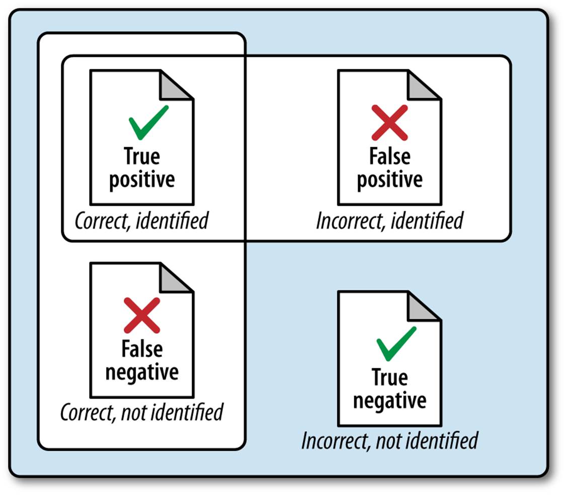
Figure 5-7. The intuition behind true positives, false positives, true negatives, and false negatives from the standpoint of predictive analytics
To put all of this into perspective, let’s consider the sentence “Mr. Green killed Colonel Mustard in the study with the candlestick” one last time and assume that an expert has determined that the key entities in the sentence are “Mr. Green,” “Colonel Mustard,” “study,” and “candlestick.” Assuming your algorithm identified these four terms and only these four terms, you’d have four true positives, zero false positives, five true negatives (“killed,” “with,” “the,” “in,” “the”), and zero false negatives. That’s perfect precision and perfect recall, which yields an F1 score of 1.0. Substituting various values into the precision and recall formulas is straightforward and a worthwhile exercise if this is your first time encountering these terms.
NOTE
What would the precision, recall, and F1 score have been if your algorithm had identified “Mr. Green,” “Colonel,” “Mustard,” and “candlestick”?
Many of the most compelling technology stacks used by commercial businesses in the NLP space use advanced statistical models to process natural language according to supervised learning algorithms. Given our discussion earlier in this chapter, you know that a supervised learning algorithm is essentially an approach in which you provide training samples that comprise inputs and expected outputs such that the model is able to predict the tuples with reasonable accuracy. The tricky part is ensuring that the trained model generalizes well to inputs that have not yet been encountered. If the model performs well for training data but poorly on unseen samples, it’s usually said to suffer from the problem of overfitting the training data. A common approach for measuring the efficacy of a model is called cross-validation. With this approach, a portion of the training data (say, one-third) is reserved exclusively for the purpose of testing the model, and only the remainder is used for training the model.
Closing Remarks
This chapter introduced the fundamentals of unstructured data analytics, and demonstrated how to use NLTK and put together the rest of an NLP pipeline to extract entities from text. The emerging field of understanding human language data is incredibly interdisciplinary and still quite nascent despite our collective attempts, and nailing the problem of NLP for most of the world’s most commonly spoken languages is arguably the problem of this century (or at least the first half of it).
Push NLTK to its limits, and when you need more performance or quality, consider rolling up your sleeves and digging into some of the academic literature. It’s admittedly a daunting task at first, but a truly worthy problem if you are interested in tackling it. There’s only so much that one chapter out of any book can teach you, but the possibilities are vast, open source toolkits are a good starting point, and there’s a bright future ahead for those who can master the science and art of processing human language data.
NOTE
The source code outlined for this chapter and all other chapters is available at GitHub in a convenient IPython Notebook format that you’re highly encouraged to try out from the comfort of your own web browser.
Recommended Exercises
§ Adapt the code from this chapter to collect a few hundred high-quality articles or blog posts from the Web and summarize the content.
§ Build a hosted web app with a toolkit such as Google App Engine to build an online summarization tool. (Given that Yahoo! recently acquired a company called Summly that summarizes news for readers, you may find this exercise particularly inspiring.)
§ Consider using NLTK’s word-stemming tools to try to compute (entity, stemmed predicate, entity) tuples, building upon the code in Example 5-9.
§ Look into WordNet, a tool that you’ll undoubtedly run into sooner rather than later, to discover additional meaning about predicate phrases you will encounter during NLP.
§ Visualize entities extracted from text with a tag cloud.
Try writing your own end-of-sentence detector as a deterministic parser based upon logic you can encode as rules in if-then statements and compare it to the facilities in NLTK. Is it appropriate to try to model language with deterministic rules?
§ Use Scrapy to crawl a small sample of news articles or blog posts and extract the text for processing.
§ Explore NLTK’s Bayesian classifier, a supervised learning technique that can be used to label training samples such as documents. Can you train a classifier to label documents as “sports,” “editorial,” and “other” from a small crawl with Scrapy? Measure your accuracy as an F1 score.
§ Are there situations in which a harmonic mean between precision and recall is not desirable? When might you want higher precision at the cost of recall? When might you want higher recall at the cost of precision?
§ Can you apply the techniques from this chapter to Twitter data? The GATE Twitter part-of-speech tagger and Carnegie Mellon’s Twitter NLP and Part-of-Speech Tagging libraries make a great starting point.
Online Resources
The following list of links from this chapter may be useful for review:
§ The Automatic Creation of Literature Abstracts
§ “Bag of words” model
§ Bayesian classifier
§ BeautifulSoup
§ Boilerplate Detection Using Shallow Text Features
§ Breadth-first search
§ Carnegie Mellon’s Twitter NLP and part-of-speech tagger
§ Common Crawl Corpus
§ Confidence interval
§ d3-cloud GitHub repository
§ Depth-first search
§ GATE Twitter part-of-speech tagger
§ Hosted version of boilerpipe
§ HTML5
§ Microdata
§ NLTK book
§ Penn Treebank Project
§ python-boilerpipe
§ Scrapy
§ Supervised machine learning
§ Thread pool
§ Turing Test
§ Unsupervised Multilingual Sentence Boundary Detection
§ WordNet
[17] Throughout this chapter, the phrase human language data refers to the object of natural language processing and is intended to convey the same meaning as natural language data or unstructured data. No particular distinction is intended to be drawn by this choice of words other than its precision in describing the data itself.
[18] A homonym is a special case of a homograph. Two words are homographs if they have the same spelling. Two words are homonyms if they have the same spelling and the same pronunciation. For some reason, homonym seems more common in parlance than homograph, even if it’s being misused.
[19] Treebank is a very specific term that refers to a corpus that’s been specially tagged with advanced linguistic information. In fact, the reason such a corpus is called a treebank is to emphasize that it’s a bank (think: collection) of sentences that have been parsed into trees adhering to a particular grammar.
[20] More precisely, F1 is said to be the harmonic mean of precision and recall, where the harmonic mean of any two numbers x and y is defined as:
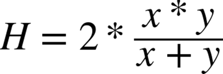
You can read more about why it’s the “harmonic” mean by reviewing the definition of a harmonic number.
All materials on the site are licensed Creative Commons Attribution-Sharealike 3.0 Unported CC BY-SA 3.0 & GNU Free Documentation License (GFDL)
If you are the copyright holder of any material contained on our site and intend to remove it, please contact our site administrator for approval.
© 2016-2026 All site design rights belong to S.Y.A.