Pro Office for iPad: How to Be Productive with Office for iPad (2014)

Chapter 7. Getting Started with Excel for iPad

In this chapter, you will get up and running with Excel for iPad. First, the chapter will briefly cover the app’s features and its limitations so that you know what’s there and what’s missing. After that, the chapter will show you how to create a new workbook and navigate the Excel interface. You will also learn how to enter data in a worksheet—by typing, by pasting, or by using the Fill feature—and how to customize Excel’s view to suit your preferences.

Understanding Excel for iPad’s Features and Limitations

As you’d probably expect, Excel for iPad is a more compact app than Excel for Windows and Excel for the Mac, the two desktop versions of Excel. Excel for iPad provides all the features you need to create and edit the most widely used types of workbooks, including about 9 in 10 of the massive range of functions that Excel supports.

Note Microsoft has added various features to Excel for iPad since launching the app, and is continuing to add features, so the details in this section may no longer be accurate by the time you read it. For example, soon after the first release, Microsoft added printing, improved support for external keyboards, and support for PivotTables whose source data is in the same workbook. So it is a good idea to update Excel on your iPad to the latest version, either by running the App Store app on your iPad and looking on the Updates tab or by using iTunes on your computer.

This section first discusses the features that Excel has and the features it lacks, then explains briefly what happens to workbook content that Excel for iPad doesn’t support.

Which Features Does Excel for iPad Have and Lack?

Excel for iPad enables you to perform all the essential actions with workbooks. You can create a new workbook, save it either online (on OneDrive or SharePoint) or on your iPad; you can open and close existing workbooks, edit them, print them, and save changes; and you can duplicate a workbook or restore a workbook to an earlier version to recover from mishaps or unfortunate edits.

At this writing, Excel for iPad is missing or has only partial support for various major features that the desktop versions of Excel offer. Here is a list of the main features:

· Templates: Excel for iPad enables you to create workbooks based on the range of templates that come with the app, but you can’t create a workbook based on a template of your own. Excel for iPad also cannot create templates yet.

· Views: The desktop versions of Excel enable you to switch between Normal view and Page Layout view as needed. By contrast, Excel for iPad has only a single view, a layout view that shows objects on screen as closely as possible to how they will appear in either a printout or a PDF file.

· Outlines: The desktop versions of Excel enable you to group rows or columns to create collapsible outlines. This feature is especially useful with large worksheets in which it is hard to see the wood for the trees. Excel for iPad doesn’t have this feature.

· Advanced charts and sparklines: Excel for iPad has good support for charts, but it doesn’t offer all the chart types that the desktop versions of Excel have. Excel for iPad also doesn’t have sparklines, mini-charts that you can insert in a single cell.

· Track Changes and protection: The desktop versions of Excel enable you to track changes made in a workbook and to protect worksheets or entire workbooks against unauthorized changes. Excel for iPad doesn’t have these capabilities; at this writing, its only review tool is comments.

· What-if analysis and validation: Excel for iPad doesn’t have advanced data tools such as what-if analysis and data validation.

· External data: Excel for iPad cannot connect to external data sources as the desktop versions can.

· SmartArt: Excel for iPad doesn’t have SmartArt diagrams, which you can use in the desktop versions to create process diagrams, list diagrams, and relationship diagrams.

· Conditional formatting: Excel for iPad doesn’t offer conditional formatting. This is formatting that changes depending on the conditions that you specify. For example, you can use conditional formatting to apply striking formatting to suspiciously high values so that they jump out at you.

· Macros and VBA: Excel for iPad doesn’t have the Visual Basic for Applications (VBA) programming language, which enables you to automate tasks using macros and user forms (custom dialog boxes).

What Happens to Content That Excel for iPad Does Not Support?

When you open a workbook that contains items that Excel for iPad doesn’t support, the app deals with them as smartly as possible. Excel for iPad correctly displays many items that it doesn’t enable you to create, and it even lets you edit them. For example, if you open a workbook that contains sparklines, Excel for iPad not only displays them correctly but also updates the sparklines if you change the values on which they are based; however, you cannot change the sparkline type or the range of cells it uses.

If a workbook contains data that Excel for iPad can’t display, it leaves that content unchanged in the file so that it is still there when you open the workbook in a desktop version of Excel. For example, Excel for iPad leaves VBA code untouched when you edit a workbook and save it.

Creating a New Workbook on Your iPad

To create a new workbook on your iPad, tap the New button on the file management screen, and then tap the button for the appropriate template on the New screen (see Figure 7-1).

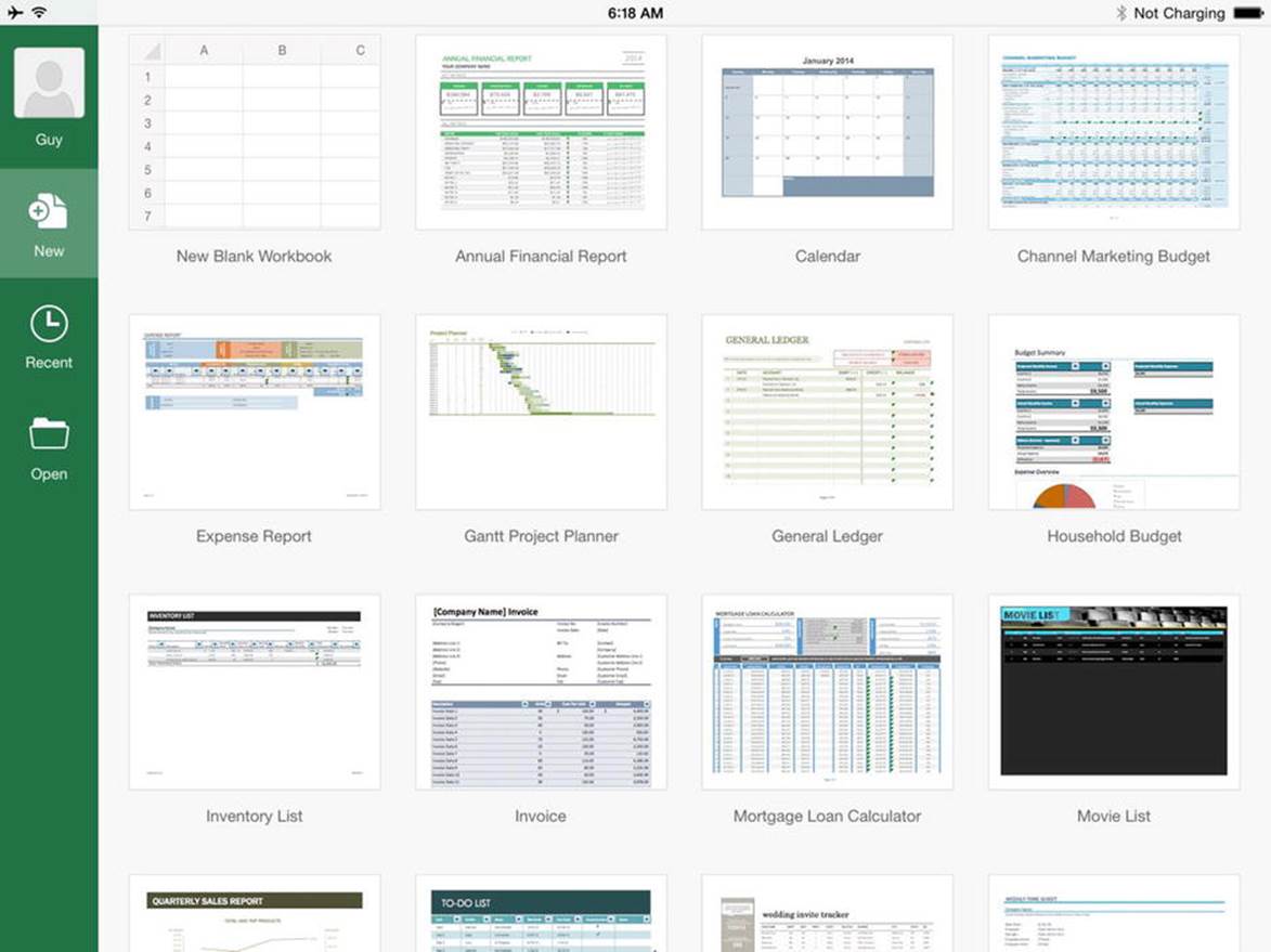
Figure 7-1. On the New screen, tap the template for the type of workbook you want to create

Tap the New Blank Workbook button if you want to create a workbook with no contents. This is good when you want to create a workbook from scratch or when you’re coming to grips with Excel.

Otherwise, tap the template that looks most suitable for the type of workbook you want to create. Excel for iPad provides a good range of templates, ranging from business-oriented templates such as the Annual Financial Report template and the Channel Marketing Report template to personal templates such as the Movie List template and the Wedding Invite Tracker template. But you can adapt any template as needed, so don’t feel constrained by the names.

Navigating the Excel Interface

Once you’ve created a workbook, you’ll see the Excel interface (see Figure 7-2). The following list explains the main elements in the Excel interface.

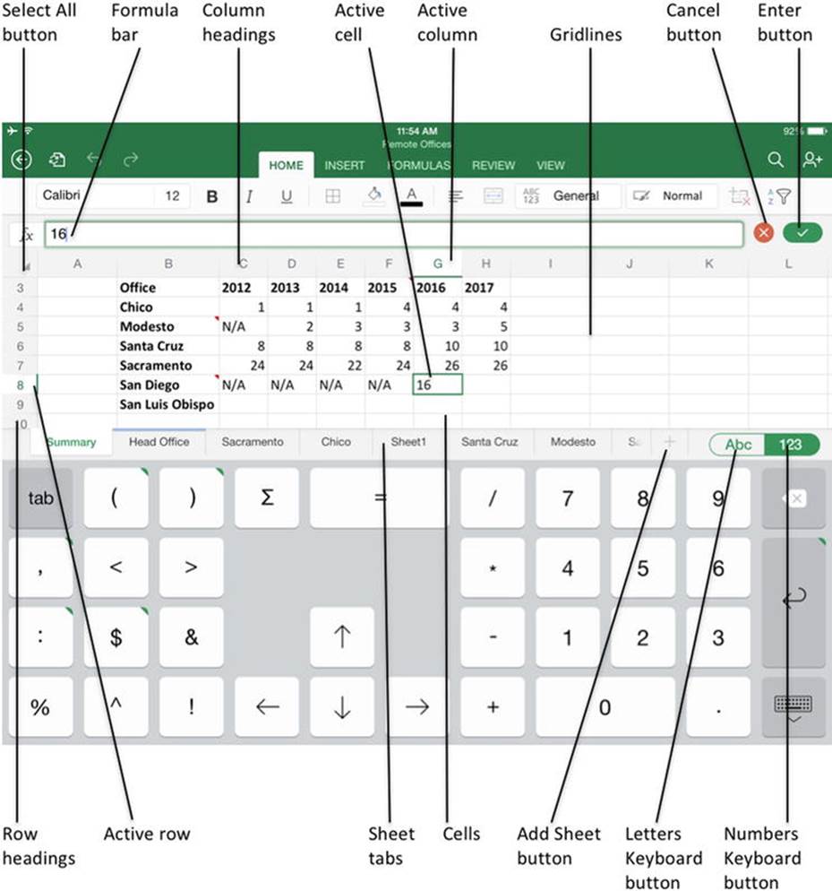
Figure 7-2. The Excel interface with a cell open for editing

Apart from the Ribbon, which you know all about already, these are the main elements of the Excel screen:

· Formula bar: This is the bar directly below the Ribbon. This bar shows the data or formula in the active cell. It is where you enter and edit data.

· Enter button: This is the green button with the white check mark that appears at the right end of the Formula bar when you are entering or editing the data in a cell. Tap this button to enter what you have typed, or the edits you have made, and to close the cell for editing.

· Cancel button: This is the red circle with the white cross that appears to the left of the Enter button at the right end of the Formula bar. You tap this button to cancel entering your text or edits and to close the cell for editing. Canceling out of a cell returns its contents (if any) to how they were before.

· Row headings: These are the numbers at the left side of the screen that identify each row. The first row is 1, the second row 2, and so on.

· Column headings: These are the letters at the top of the worksheet grid that identify the columns. The first column is A, the second column is B, and so on.

· Cells: These are the boxes formed by the intersections of the rows and columns. Each cell is identified by its column letter and row number. For example, the first cell in column A is cell A1, and the second cell in column B is cell B2.

· Gridlines: These are the light-gray lines that separate the cells. Excel displays the gridlines by default so that you can see where each cell falls. You can turn off the gridlines by displaying the View tab of the Ribbon and setting the Gridlines switch to the Off position.

· Active cell: This is the cell you’re working in. Excel displays a heavy green rectangle around the active cell.

· Active row: This is the row that contains the active cell. Excel displays the row heading for the active row with a lighter gray background, the number in green rather than gray, and a green line on the right side of the heading to help you pick out the active row easily.

· Active column: This is the column that contains the active cell. As with the active row, Excel displays the column heading for the active row with a lighter gray background, the number in green rather than gray, and a green line at the bottom for easy identification.

· Select All button: Tap this button at the intersection of the row headings and column headings to select all the cells in the worksheet.

· Sheet tabs: To display a worksheet or a chart sheet, you tap its sheet tab on the Sheet tab bar.

· Add Sheet button: Tap this button to add a new worksheet after the current sheet.

· Letters Keyboard button: Tap this button to display the letters keyboard. You will learn about the Excel keyboard later in this chapter.

· Numbers Keyboard button: Tap this button to display the numbers keyboard.

Navigating Workbooks and Worksheets

Each workbook consists of one or more worksheets or other sheets, such as chart sheets, macro sheets, or dialog sheets. To display the sheet you want to view, tap its tab in the Sheet Tabs bar at the bottom of the Excel screen. If the sheet’s tab isn’t visible, scroll the Sheet Tabs bar left or right until you can see the right tab.

Note A chart sheet is a separate sheet that contains a chart. A macro sheet is a sheet that contains macros, sequences of commands. A dialog sheet is a sheet that contains custom dialog boxes for purposes such as controlling the running of macros. Macro sheets and dialog sheets are for the desktop versions of Excel.

Each worksheet contains 16,384 columns and 1,048,576 rows, giving a grand total of 17,179,869,184 cells. Normally, you’ll use only a small number of these cells—perhaps a few hundred or a few thousand—but there’s plenty of space should you need it for large worksheets.

Each column is identified by one, two, or three letters:

· The first 26 columns use the letters A to Z.

· The next 26 columns use AA to AZ, the following 26 BA to BZ, and so on.

· When the two-letter combinations are exhausted, Excel uses three letters: AAA, AAB, and so on.

Each row is identified by a number, from 1 up to 1048576.

Each cell is identified by its column lettering and its row number. For example, the cell at the intersection of column A and row 1 is cell A1, and the cell at the intersection of column ZA and row 2256 is ZA2256.

Moving the Active Cell

In Excel, you usually work in a single cell at a time. That cell is called the active cell and receives the input from the keyboard. You move the active cell by tapping the cell that you want to make active. To make a cell active and open it for editing, you double-tap it. If the cell you want to open for editing is already the active cell, tap the Formula bar to open it for editing. (You can also double-tap the active cell if you prefer.)

When you have opened the active cell for editing, you can tap the arrow buttons on the numbers keyboard to move from cell to cell. Tap the Up arrow button to move the active cell up to the cell in the next row, tap the Right arrow button to move the active cell to the next column, and so on.

If you connect a hardware keyboard to your iPad, you can move the active cell by using the keys and keyboard shortcuts explained in Table 7-1.

Table 7-1. Keyboard Shortcuts for Moving the Active Cell

Tip Tap the Excel title bar to scroll up quickly to the top rows of the active worksheet.

Selecting Cells and Ranges

To work with a single cell, you simply tap it. When you need to affect multiple cells at once, you select the cells. For example, you can select multiple cells so that you can apply formatting to them.

Excel calls the selection of cells a range. In Excel, a range can consist of either a rectangle of contiguous cells or various cells that aren’t next to each other. At this writing, Excel for iPad enables you to select only ranges of contiguous cells, and only one range at a time, unlike the desktop versions of Excel, which let you select ranges of noncontiguous cells and multiple ranges at once.

To select a range, tap the cell at one corner of the range to make it the active cell. Then tap the corner handle on the active cell and drag it until the selection encompasses all the cells you want in the range (see Figure 7-3).

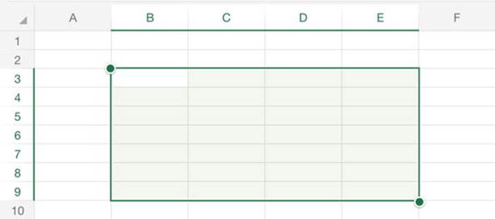
Figure 7-3. To select a range, tap any corner handle on the active cell and drag until the selection encompasses the cells you want

Tip If you connect a hardware keyboard to your iPad, you can select text by holding down the Shift key and pressing the keys or shortcuts shown in Table 7-1. For example, hold down the Shift key and press the Right arrow key to extend the selection to the right by one column, or press the Down arrow key to extend the selection to the next row. The Command+Up arrow keyboard shortcut (select to the first row) and the Command+Left arrow shortcut (select to the first column) tend to be more useful than the Command+Down arrow shortcut (select to the last row) and the Command+Right arrow shortcut, which usually select galaxies of emptiness.

To select an entire row, tap its row heading. Similarly, to select an entire column, tap its column heading.

To deselect the range you’ve selected, tap any cell either inside or outside the range.

Entering Data in a Worksheet

You can enter data in your worksheets by typing it, by pasting it, or by using drag and drop to move or copy it. Excel also includes a feature called Fill that automatically fills in series data for you based on the input you’ve provided.

Opening a Cell for Editing

Before you can enter data in a cell using the onscreen keyboard, you need to open the cell for editing. To do so, you double-tap the cell. Excel automatically displays the onscreen keyboard so that you can enter the data with it.

Note When you have a hardware keyboard connected to your iPad, you can simply select the cell and start typing to open the cell for editing and enter data in it. Entering data this way overwrites any existing contents in the cell. (If you’ve used a desktop version of Excel, you’ll be familiar with this behavior.) If you double-tap a cell, Excel opens it for editing but doesn’t display the onscreen keyboard (because the hardware keyboard is there). You can then edit the existing contents of the cell.

Meeting Excel’s Numbers Keyboard

As well as the default iOS keyboards, Excel for iPad has a custom onscreen numbers keyboard to help you enter data more quickly. Tap the 123 button at the right end of the Sheet Tabs bar to display the numbers keyboard (see Figure 7-4), which is largely self-explanatory except for these features:

· SUM key: Tap this key to enter the SUM() function in the active cell. SUM() is the most widely used function, so it’s great to have it at your fingertip.

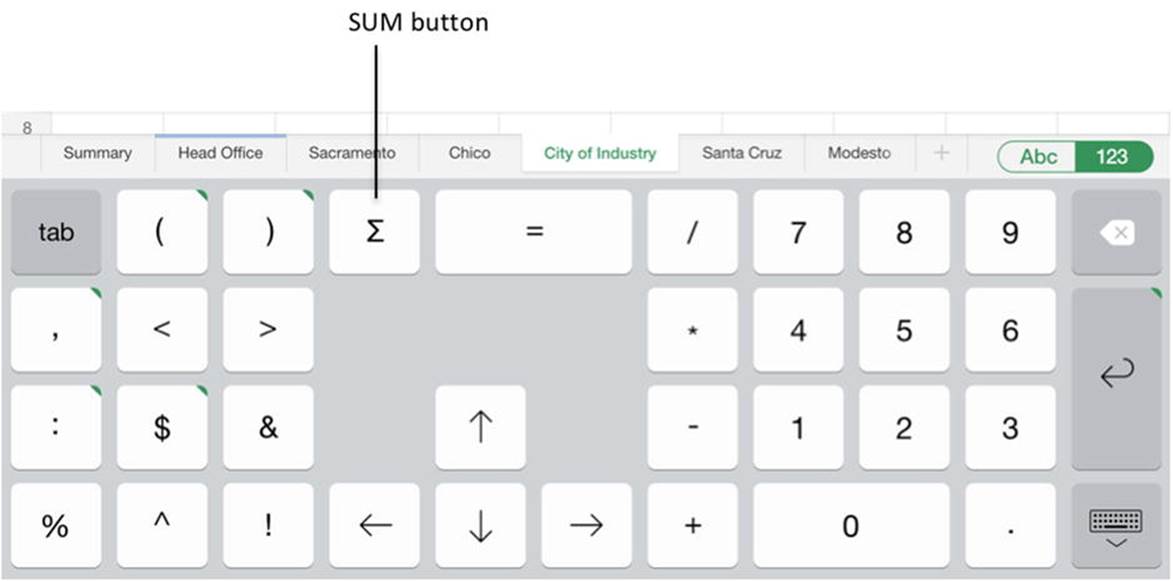
Figure 7-4. Excel provides a customized numbers keyboard to enable to you enter data, functions, and formulas more easily

· Green-triangle keys: The green triangles in the upper-right corner of a key indicate that the key has a pop-up panel with alternate characters. Table 7-2 shows you the alternate characters available. Tap and hold the key to display the pop-up panel, slide your finger to the character you want, and then lift your finger.

Table 7-2. Alternate Keys on the Number Keyboard

· Tab key: Tap this key to move the active cell one column to the right.

· Arrow keys: Tap an arrow key to move the active cell one column or row in the direction shown on the key.

Note You can use the standard iOS numbers and symbols keyboards if you prefer. To display the numbers keyboard, tap the .?123 button on the letters keyboard as usual; and to display the symbols keyboard, tap the #+= button on the numbers keyboard.

Typing Data in a Cell

The most straightforward way to enter data is to type it into a cell. Double-tap the cell to make it active and open it for editing. You can then start typing on the onscreen keyboard, which Excel displays automatically.

When you’ve finished typing the contents of the cell, move to another cell in any of these ways:

· Tap the Return key: Excel moves the active cell to the next cell below the current cell.

· Tap the Tab key: Excel moves the active cell to the next cell to the right of the current cell.

· Tap another cell: Excel moves the active cell to the cell you tap.

· Tap an arrow key: Excel moves the active cell to the next cell in the direction of the arrow. For example, tap the Right arrow key to move the active cell to the next cell to the right.

Excel automatically opens the cell you move to, so you don’t need to double-tap it.

When you finish your editing session, tap the Enter button at the right end of the Formula bar to accept the current entry and close the cell for editing. Excel hides the onscreen keyboard.

Editing a Cell’s Contents

When you need to edit the existing contents of a cell, double-tap the cell to open it for editing. Excel displays the cell’s contents in the Formula bar (see Figure 7-5), and you can edit them there using the onscreen keyboard, which appears automatically.

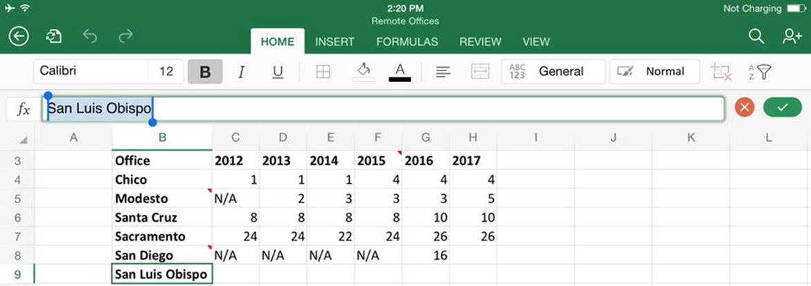
Figure 7-5. Double-tap a cell to open it for editing. You can then edit the cell’s contents in the Formula bar

When you finish editing the cell, either move to another cell you want to edit as described in the previous section, or tap the Enter button to close the cell for editing.

Entering Data Quickly Using the Fill Feature

When you need to fill in a series of data, see if Excel’s Fill feature can enter it for you. To use Fill, you enter the base data for the series in one or more cells. You then select the cells, activate Fill, and then drag the Fill handle in the direction you want to fill. Fill checks your base data, works out what the other cells should contain, and fills it in for you.

To get the hang of Fill, try the following example on a blank worksheet in a practice workbook. If you’re currently working on a valuable workbook, tap the Back button to return to the file management screen, tap the New button, and then tap the New Blank Workbook button to create a new blank workbook.

The first example uses the days of the week. Follow these steps.

1. Double-tap cell A1 to open the cell for editing.

2. Type Monday in the cell.

3. Tap the Enter button to close the cell for editing. The cell remains active.

4. Tap the cell again to display the Edit menu (see Figure 7-6).

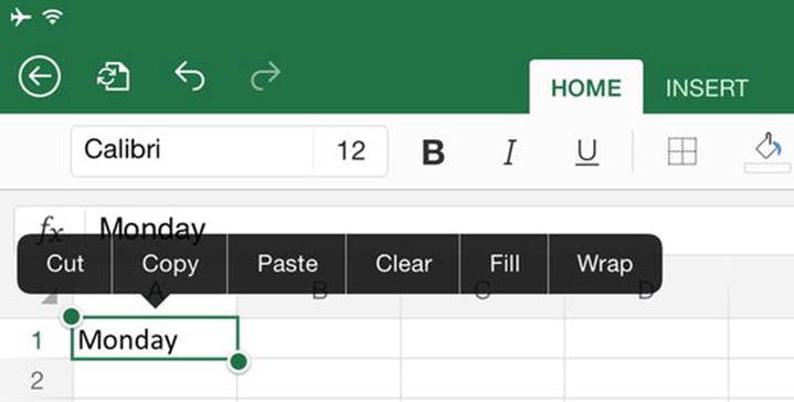
Figure 7-6. Tap the active cell to display the Edit menu, and then tap the Fill button to turn on Fill

5. Tap the Fill button on the Edit menu to activate the Fill feature. Fill arrows (green circles containing white arrows) appear showing the directions in which you can drag (see Figure 7-7).

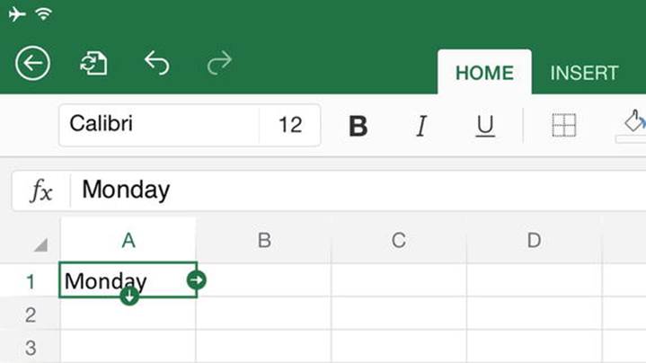
Figure 7-7. The Fill arrows indicate that Fill is active

6. Tap a Fill arrow and drag it to select the range of cells you want to fill with data (see Figure 7-8).

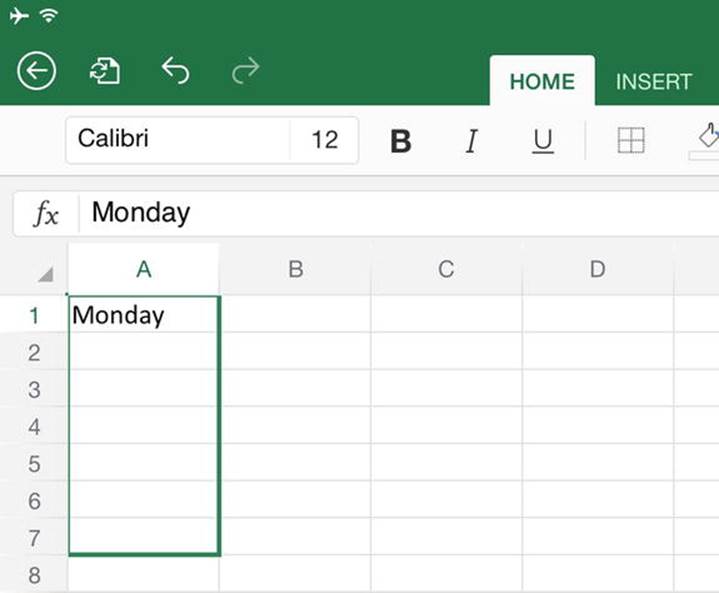
Figure 7-8. Drag a Fill arrow to select the cells you want to fill

7. Lift your finger from the screen. Excel fills the cells with data—in this case, the days Tuesday through Sunday (see Figure 7-9).

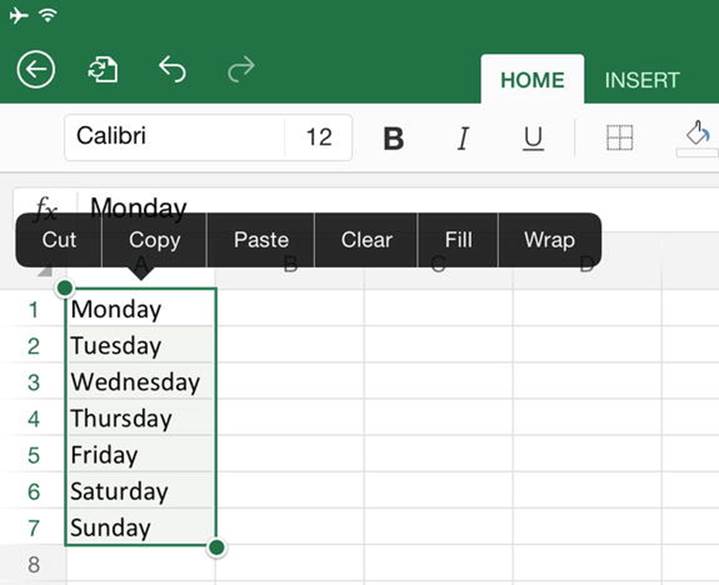
Figure 7-9. Excel fills the cells with data when you lift your finger

Here are three examples of data you can complete using the Fill feature:

· Months and years: Enter January in a cell and use the Fill feature to enter the remaining months. Or enter 2015 in one cell, 2016 in the next cell, and use Fill to fill in the following years.

· Date series: Enter a date such as 5/13/15 in one cell, 5/20/15 in another cell, and use Fill to fill in the following dates at one-week intervals: 5/27/15, 6/3/15, and so on. (How these dates appear depends on the date format set for the cells.)

· Linear trend: Enter 5 in one cell and 10 in the cell below it. Select the two cells, turn on Fill, and drag the Fill handle to select the cells below the cell containing 10. Fill enters the numbers 15, 20, 25, and so on in the cells, following the linear trend suggested by the first two cells.

Caution If you’re used to filling in complex series with the AutoFill feature in the desktop versions of Excel, check through your Fill results carefully on the iPad. At this writing, the Fill feature on Excel for iPad cannot fill in series such as growth trends, so you may get some unwelcome surprises.

Pasting Data into a Worksheet

If the data you need to add to a worksheet is already in another document, you can copy it and paste it into the worksheet. Follow these steps.

1. In the source document and app, select the data and copy it to the Clipboard.

2. Switch to Excel if the source is another app.

3. Tap the upper-left cell in the destination range to make it active.

4. Tap the active cell to display the Edit menu.

5. Tap the Paste button. Excel pastes the data using default settings, which includes the source formatting (if any).

6. If you need to change what you’ve pasted, tap the Paste Options button below and to the right of the lower-right cell of the pasted material. The Paste Options pop-up menu appears (see Figure 7-10).

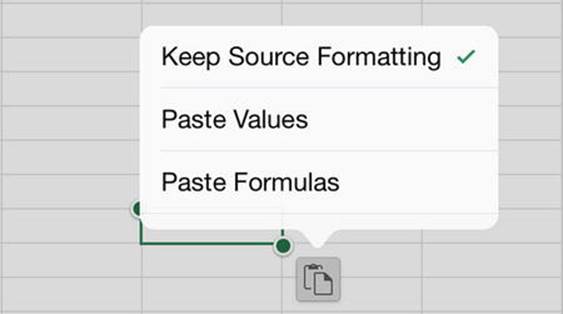
Figure 7-10. To change what you’ve pasted, tap the Paste Options button, and then tap the button for the appropriate paste option

7. Tap the button for the paste option you want to use. Your options vary depending on what you’ve pasted, but you’ll frequently see some of the following options:

o Keep Source Formatting: Tap this button to preserve the source formatting of what you pasted, keeping the item looking as it did when you copied it.

o Use Destination Theme: After pasting an object, such as a chart or a shape, tap this button to apply the formatting theme of the destination range to the object.

o Paste Values: Tap this button to paste the values with no formatting.

o Paste Formulas: Tap this button to paste the formulas and constants without formatting.

o Paste as Picture: Tap this button to paste in the copied object as a picture rather than as editable text.

Moving Data with Cut and Paste and Drag and Drop

When you need to move data to a different location, you can use either cut and paste or drag and drop.

To use cut and paste, select the data in its source and copy it to the Clipboard. Then tap the upper-left cell in the destination range, tap again to display the Edit menu, and tap the Paste button.

To move data with drag and drop, follow these steps.

1. Select the cell or range you want to move.

2. Tap and hold the selection until it becomes mobile.

3. Drag the selection to the destination (see Figure 7-11) and then lift your finger.

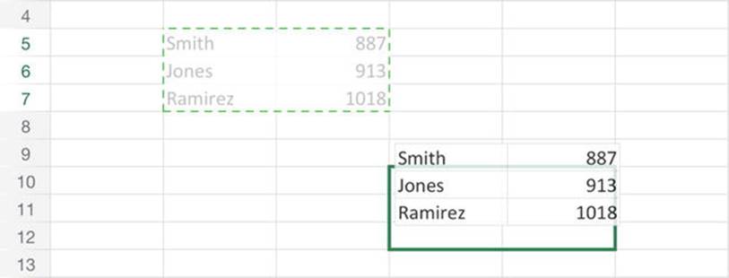
Figure 7-11. You can use drag and drop to move a selection to a different location in the same worksheet

Creating Tables

When you create a worksheet that contains many related items in a single range, you may benefit from creating a table. For example, if you need to record data such as purchase orders or customer details, you can put each item in a separate row and then create a table that contains all the rows. The table enables you to treat each row as a record and to sort and filter the rows to show the information you need.

Note Some of the templates in Excel for iPad contain tables already set up for you to use.

To create a table, follow these steps.

1. Open the workbook you want to use. Create a new workbook if necessary.

2. If you need to add a worksheet, click the New Sheet button. Name the worksheet so that you can easily identify it.

3. Type the headings for the table. For example, if the table will contain customer names and addresses, you’d type fields such as Last Name, First Name, Middle Initial, Title, Address 1, and so on.

4. Tap the row heading for the headings row and then apply formatting to the row to distinguish it from the following rows. For example, tap the Bold button on the Home tab of the Ribbon to apply boldface.

5. Enter the first record in the first row below the headings. (If you don’t have records yet, enter sample data—but remember to remove it after creating the table.) You can enter multiple records if you want, but you don’t need to. Add to this row any number formatting or other formatting the table’s cells will need. The rows you add subsequently will pick up the formatting from this row.

6. Select the headings and the row of data below them. If you’ve entered multiple records, select them all.

7. Tap the Insert tab of the Ribbon to display its controls (see Figure 7-12).

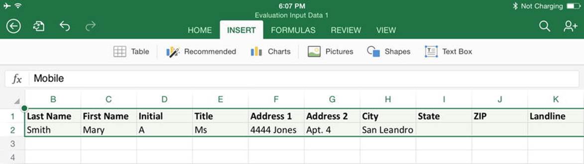
Figure 7-12. Tap the Table button on the Insert tab of the Ribbon to convert the selected headings and data into a table

8. Tap the Table button. Excel converts the headings and data into a table and adds the Table tab to the Ribbon (see Figure 7-13).

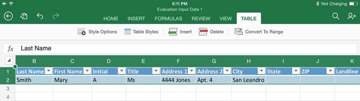
Figure 7-13. Each heading cell in the table becomes a pop-up menu that you can use to sort and filter the table

Note See Chapter 9 for sorting and filtering in Excel worksheets and tables.

You can now add further records to the table. As long as you put the next record in the row immediately under the last existing row, Excel automatically adds it to the table. You can also add rows within the table if you prefer by tapping the Insert button on the Table tab of the Ribbon and then tapping the appropriate item on the Insert pop-up panel (see Figure 7-14).

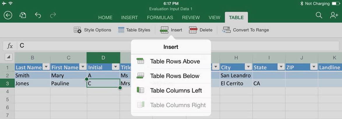
Figure 7-14. You can insert rows inside the table by tapping the appropriate button on the Insert pop-up panel

Note See the section “Applying Table Formatting” in Chapter 8 for details on how to format tables with table styles.

Setting Up Your Preferred View

Excel enables you to display or hide several elements of the user interface to make the app look and behave the way you want it to. You can also freeze the panes in a worksheet so that specific rows and columns remain visible no matter how far down or how far across the worksheet you scroll.

Choosing Which Onscreen Items to Display

To choose which onscreen items to display, tap the View tab of the Ribbon to display its controls (see Figure 7-15). You can then set the following four switches to the On position or to the Off position, as needed:

· Formula Bar: You can hide the Formula bar when you have finished entering data and you need more space on screen. Excel automatically displays the Formula bar if you open a cell for editing.

Figure 7-15. On the View tab of the Ribbon, you can toggle the display of the Formula bar, Sheet tabs, row and column headings, and gridlines

· Sheet Tabs: You can hide the sheet tabs to get more space on screen or to hide the other worksheets while displaying the worksheet to others on your iPad.

· Headings: You can hide the row and column headings when you don’t want others to see them. The usual reason for hiding the headings is to prevent others from seeing that you have hidden some rows, columns, or both.

· Gridlines: You can hide the gridlines if your worksheet looks better without them. If you want gridlines on some cells but not on the rest of the worksheet, use the Borders button on the Home tab of the Ribbon to apply borders to those cells.

Freezing Panes

To keep your data headings on screen when you scroll down or to the right on a large worksheet, you can freeze the heading rows and columns in place. For example, if you have headings in column A and row 1, you can freeze column A and row 1 so that they remain on screen.

You can quickly freeze the first column, the top row, or your choice of rows and columns:

· Freeze the first column: Tap the Freeze Panes button, and then tap the Freeze First Column button on the Freeze Panes pop-up panel (see Figure 7-16).

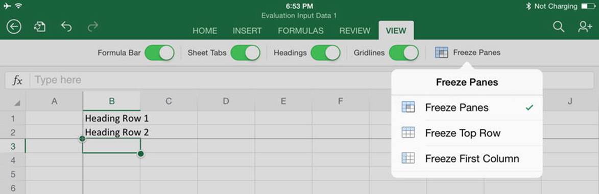
Figure 7-16. From the Freeze Panes pop-up panel, you can freeze the top row, the first column, or your choice of rows and columns

· Freeze the first row: Tap the Freeze Panes button, and then tap the Freeze Top Row button on the Freeze Panes pop-up panel.

· Freeze your choice of rows and columns: Tap the cell below the row and to the right of the column you want to freeze. For example, to freeze the top two rows and column A, tap cell B3. Then tap the Freeze Panes button and tap the Freeze Panes button on the Freeze Panes pop-up panel.

Summary

In this chapter, you got off to a running start with Excel for iPad. You now know what features and limitations the app has compared to the desktop versions. You can create workbooks, navigate the Excel interface, and enter data in a worksheet using several essential techniques. You also learned how to use the View controls to make Excel look the way you prefer.

In the next chapter, you will learn how to build worksheets and format them to look the way you want.