Discovering Modern C++. An Intensive Course for Scientists, Engineers, and Programmers(2016)
Chapter 4. Libraries
“God, grant me the serenity to accept the things I cannot change, The courage to change the things I can, And the wisdom to know the difference”
—Reinhold Niebuhr
We as programmers need similar strengths. We have great visions of what our software should accomplish, and we need very strong Courage to make this happen. Nonetheless, a day has only 24 hours and even hardcore geeks eat and sleep sometimes. As a consequence, we cannot program everything we dream of (or are paid for) by ourselves and have to rely on existing software. Then we have to Accept what this software provides us by implementing interfaces with appropriate pre- and post-processing. The decision whether to use existing software or write a new program requires all our Wisdom.
Actually, it even requires some prophetic powers to rely on software without having years of experience with it. Sometimes, packages work well at the beginning, and once we build a larger project on top of it, we may experience some serious problems that cannot be compensated for easily. Then we might realize painfully that another software package or an implementation from scratch would have been the better option.
The C++ standard library might not be perfect, but it is designed and implemented very carefully so that we can prevent such bad surprises. The components of the standard library pass the same thorough evaluation process as the features of the core language and guarantee the highest quality. The library standardization also assures that its classes and functions are available on every compliant compiler. We already introduced some library components before, like initializer lists in §2.3.3 or I/O streams in §1.7. In this chapter, we will present more library components that can be very useful for the programming scientist or engineer.
A comprehensive tutorial and reference for the standard library in C++11 is given by Nicolai Josuttis [26]. The fourth edition of Bjarne Stroustrup’s book [43] covers all library components as well, although in a little less detail.
Furthermore, there are many scientific libraries for standard domains like linear algebra or graph algorithms. We will briefly introduce some of them in the last section.
4.1 Standard Template Library
The Standard Template Library (STL) is the fundamental generic library for containers and algorithms. Every programmer should know it and use it when appropriate instead of reinventing the wheel. The name might be a bit confusing: most parts of the STL as created by Alex Stepanov and David Musser became part of the C++ standard library. On the other hand, other components of the standard library are also implemented with templates. To make the confusion perfect, the C++ standard associates a library name with each library-related chapter. In the 2011 and 2014 standards, the STL is contained in three such chapters: Chapter 23 Containers library, Chapter 24 Iterators library, and Chapter 25 Algorithms library (the latter also contains part of the C library).
The Standard Template Library doesn’t only provide useful functionality but also laid the foundation of a programming philosophy that is incomparably powerful in its combination of reusability and performance. The STL defines generic container classes, generic algorithms, and iterators. Online documentation is provided under www.sgi.com/tech/stl. There are also entire books written about the usage of STL, so we can keep it short here and refer to these books. For instance, Matt Austern—an STL core implementer—wrote an entire book exclusively on it: [3]. Josuttis’s library tutorial dedicates around 500 pages to the STL only.
4.1.1 Introductory Example
Containers are classes whose purpose is to contain objects (including containers and containers of containers and so on). The classes vector and list are examples of STL containers. Each of these class templates is parameterized by an element type. For example, the following statements create a double and an int vector:
std::vector<double> vec_d;
std::vector<int> vec_i;
Note that the STL vectors are not vectors in the mathematical sense as they don’t provide arithmetic operations. Therefore, we created our own vector class in various evolving implementations.
The STL also includes a large collection of algorithms that manipulate the containers’ data. The before-mentioned accumulate algorithm, for example, can be used to compute any reduction—such as sum, product, or minimum—on a list or vector in the following way:
std::vector<double> vec ; // fill the vector...
std::list<double> lst ; // fill the list...
double vec_sum = std::accumulate(begin(vec), end(vec), 0.0);
double lst_sum = std::accumulate(begin(lst), end(lst), 0.0);
The functions begin() and end() return iterators representing right-open intervals as before. C++11 introduced the free-function notation for them while we have to use the corresponding member functions in C++03.
4.1.2 Iterators
The central abstraction of the STL is Iterators. Simply put, iterators are generalized pointers: one can dereference and compare them and change the referred location as we have already demonstrated with our own list_iterator in Section 3.3.2.5. However, this simplification does not do justice to the iterators given their importance. Iterators are a Fundamental Methodology to Decouple the Implementation of Data Structures and Algorithms. In STL, every data structure provides an iterator for traversing it, and all algorithms are implemented in terms of iterators as illustrated in Figure 4–1.
Figure 4–1: Interoperability between STL containers and algorithms
To program m algorithms on n data structures, one needs in classical C and Fortran programming
m · n implementations.
Expressing algorithms in terms of iterators decreases the number to only
m + n implementations!
4.1.2.1 Categories
Not all algorithms can be used with every data structure. Which algorithm works on a given data structure (e.g., linear find or binary search) depends on the kind of iterator provided by the container. Iterators can be distinguished by the form of access:
InputIterator: an iterator concept for reading the referred entries (but only once).
OutputIterator: an iterator concept for writing to the referred entries (but only once).
Note that the ability to write doesn’t imply readability; e.g., an ostream_iterator is an STL interface used for writing to output streams like cout or output files. Another differentiation of iterators is the form of traversal:
ForwardIterator: a concept for iterators that can pass from one element to the next, i.e., types that provide an operator++. It is a refinement1 of InputIterator and OutputIterator. In contrast to those, ForwardIterator allows for reading values twice and for traversing multiple times.
1. In the sense of §3.5.
BidirectionalIterator: a concept for iterators with step-wise forward and backward traversal, i.e., types with operator++ and operator--. It refines ForwardIterator.
RandomAccessIterator: a concept for iterators to which an arbitrary positive or negative offset can be added, i.e., types that additionally provide operator[]. It refines BidirectionalIterator.
Algorithm implementations that only use a simple iterator interface (like that of InputIterator) can be applied to more data structures. Also, data structures that provide a richer iterator interface (e.g., modeling RandomAccessIterator) can be used in more algorithms.
A clever design choice of all iterator interfaces was that their operations are also provided by pointers. Every pointer models RandomAccessIterator so that all STL algorithms can be applied on old-style arrays via pointers.
4.1.2.2 Working with Iterators
![]()
All standard container templates provide a rich and consistent set of iterator types. The following very simple example shows a typical use of iterators:
using namespace std;
std::list<int> l= {3, 5, 9, 7}; // C++11
for (list<int>::iterator it= l.begin(); it != l.end(); ++it) {
int i= *it;
cout ![]() i
i ![]() endl;
endl;
}
In this first example, we limited ourselves to C++03 features (apart from the list initialization) to demonstrate that the work with iterators is nothing new to C++11. In the remainder of the section, we will use more C++11 features but the principle remains the same.
As illustrated in the code snippet, iterators are typically used in pairs, where one handles the actual iteration and the second one marks the end of the container. The iterators are created by the corresponding container class using the standard methods begin() and end(). The iterator returned by begin() points to the first element whereas end() yields an iterator pointing past the end of elements. The end iterator is only used for comparison since the attempt to access the value fails in most cases. All algorithms in STL are implemented with right-open intervals [b, e) operating on the value referred to by b until b = e. Therefore, intervals of the form [x, x) are regarded as empty.
The member functions begin() and end() preserve the constancy of the container:
• If the container object is mutable, then the methods return an iterator type referring to mutable container entries.
• For constant containers the methods return const_iterator which accesses the container entries by constant references.
Often iterator is implicitly convertible into const_iterator but you should not count on this.
Back to modern C++. We first incorporate type deduction for the iterator:
std::list<int> l= {3, 5, 9, 7};
for (auto it = begin(l), e= end(l); it != e; ++it) {
int i= *it;
std::cout ![]() i
i ![]() std::endl;
std::endl;
}
We also switched to the more idiomatic notation of free functions for begin and end that were introduced in C++11. As they are inline functions, this change doesn’t affect the performance. Speaking of performance, we introduced a new temporary to hold the end iterator since we cannot be 100 % sure that the compiler can optimize the repeated calls for the end function.
Where our first snippet used const_iterator, the deduced iterator allows us to modify the referred entries. Here we have multiple possibilities to assure that the list is not modified inside the loop. One thing that doesn’t work is const auto:
for (const auto it = begin(l), e= end(l); ...) // Error
This doesn’t deduce a const_iterator but a const iterator. This is a small but important difference: the former is a (mutable) iterator referring to constant data while the second is a constant itself so it cannot be incremented. As mentioned before, begin() and end() returnconst_iterator for constant lists. So we can declare our list to be constant with the drawback that it can only be set in the constructor. Or we define a const reference to this list:
const std::list<int>& lr= l;
for (auto it = begin(lr), e= end(lr); it != e; ++it) ...
or cast the list to a const reference:
for (auto it = begin(const_cast<const std::list<int>&>(l)),
e= end(const_cast<const std::list<int>&>(l));
it != e; ++it) ...
Needless to say, both versions are rather cumbersome. Therefore, C++11 introduced the member functions cbegin and cend returning const_iterator for both constant and mutable containers. The corresponding free functions were introduced in C++14:
for (auto it = cbegin(l); it != cend(l); ++it) // C++14
That this begin-end-based traversal pattern is so common was the motivation for introducing the range-based for (§1.4.4.3). So far, we have only used it with anachronistic C arrays and are glad now to finally apply it to real containers:
std::list<int> l= {3, 5, 9, 7};
for (auto i : l)
std::cout ![]() i
i ![]() std::endl;
std::endl;
The loop variable i is a dereferenced (hidden) iterator traversing the entire container. Thus, i refers successively to each container entry. Since all STL containers provide begin and end functions, we can traverse them all with this concise for-loop.
More generally, we can apply this for-loop to all types with begin and end functions returning iterators: like classes representing sub-containers or helpers returning iterators for reverse traversion. This broader concept including all containers is called Range, and this is not surprisingly where the name range-based for-loop originates from. Although we only use it on containers in this book it is worth mentioning it since ranges are gaining importance in the evolution of C++. To avoid the overhead of copying the container entries into i, we can create a type-deduced reference:
for (auto& i : l)
std::cout ![]() i
i ![]() std::endl;
std::endl;
The reference i has the same constancy as l: if l is a mutable/constant container (range), then the reference is mutable/constant as well. To assure that the entries cannot be changed, we can declare a const reference:
for (const auto& i : l)
std::cout ![]() i
i ![]() std::endl;
std::endl;
The STL contains both simple and complex algorithms. They all contain (often somewhere deep inside) loops that are essentially equivalent to the examples above.
4.1.2.3 Operations
The <iterator> library provides two basic operations: advance and distance. The operation advance(it, n) increments n times the iterator it. This might look like a cumbersome way to say it+n but there are two fundamental differences: the second notation doesn’t change the iterator it (which is not necessarily a disadvantage) and it works only with a RandomAccessIterator. The function advance can be used with any kind of iterator. In that sense, advance is like an implementation of += that also works for iterators that can only step one by one.
To be efficient, the function is internally dispatched for different iterator categories. This implementation is often used as an introduction for Function Dispatching, and we cannot resist sketching a typical implementation of advance:
Listing 4–1: Function dispatching in advance
template <typename Iterator, typename Distance>
inline void advance_aux(Iterator& i, Distance n, input_iterator_tag)
{
assert(n >= 0);
for (; n > 0; --n)
++i;
}
template <typename Iterator, typename Distance>
inline void advance_aux(Iterator& i, Distance n,
bidirectional_iterator_tag)
{
if (n >= 0)
for (; n > 0; --n) ++i;
else
for (; n < 0; ++n) --i;
}
template <typename Iterator, typename Distance>
inline void advance_aux(Iterator& i, Distance n,
random_access_iterator_tag)
{
i+= n;
}
template <typename Iterator, typename Distance>
inline void advance(Iterator& i, Distance n)
{
advance(i, n, typename iterator_category<Iterator>::type());
}
When the function advance is instantiated with an iterator type, the category of that iterator is determined by a type trait (§5.2.1). An object of that Tag Type determines which overload of the helper function advance_aux is called. Thus the run time of advance is constant whenIterator is a random-access iterator and linear otherwise. Negative distances are allowed for bidirectional and random-access iterators.
Modern compilers are smart enough to realize that the third argument in each overload of advance_aux is unused and that the tag types are empty classes. As a consequence, the argument passing and construction of the tag type objects are optimized out. Thus, the extra function layer and the tag dispatching don’t cause any run-time overhead. For instance, calling advance on a vector iterator boils down to generating the code of i+= n only.
The dual counterpart of advance is distance:
int i= distance(it1, it2);
It computes the distance between two iterators, i.e., how often the first iterator must be incremented to be equal to the second one. It goes without saying that the implementation is tag-dispatched as well so that the effort for random-access iterators is constant and linear otherwise.
4.1.3 Containers
The containers in the standard library cover a broad range of important data structures, are easy to use, and are quite efficient. Before you write your own containers, it is definitely worth trying the standard ones.
4.1.3.1 Vectors
std::vector is the simplest standard container and the most efficient for storing data contiguously, similar to C arrays. Whereas C arrays up to a certain size are stored on the stack, a vector always resides on the heap. Vectors provide a bracket operator and array-style algorithms can be used:
std::vector<int> v= {3, 4, 7, 9};
for (int i= 0; i < v.size(); ++i)
v[i]*= 2;
Alternatively, we can use the iterators: directly or hidden in range-based for:
for (auto& x : v)
x*= 2;
The different forms of traversal should be similarly efficient. Vectors can be enlarged by adding new entries at the end:
std::vector<int> v;
for (int i= 0; i < 100; ++i)
v.push_back(my_random());
where my_random() returns random numbers like a generator in Section 4.2.2. The STL vector often reserves extra space as illustrated in Figure 4–2 to accelerate push_back.

Figure 4–2: Memory layout of vector
Therefore, appending entries can be
• Either pretty fast by just filling already reserved space;
• Or rather slow when more memory must be allocated and all data copied.
The available space is given by the member function capacity. When the vector data is enlarged, the amount of extra space is usually proportional to the vector size, so push_back takes asymptotically constant time. Typical implementations perform two memory allocations when the vector is doubled in size (i.e., enlarged from s to ![]() at each reallocation). Figure 4–3 illustrates this: the first picture is a completely filled vector where the addition of a new entry requires a new allocation as in the second picture. After that, we can add further entries until the extra space is filled as well, as in picture three. Then new memory has to be allocated and all entries must be copied as in the fourth picture; only then a new entry can be added.
at each reallocation). Figure 4–3 illustrates this: the first picture is a completely filled vector where the addition of a new entry requires a new allocation as in the second picture. After that, we can add further entries until the extra space is filled as well, as in picture three. Then new memory has to be allocated and all entries must be copied as in the fourth picture; only then a new entry can be added.
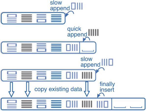
Figure 4–3: Appending vector entries
The method resize(n) shrinks or expands the vector to size n. New entries are default-constructed (or set to 0 for built-in types). Shrinking vectors with resize doesn’t release memory. This can be done in C++11 with shrink_to_fit which reduces the capacity to the actual vector size.
![]() c++11/vector_usage.cpp
c++11/vector_usage.cpp
The following simple program illustrates how a vector is set up and modified with C++11 features:
![]()
#include <iostream>
#include <vector>
#include <algorithm>
int main ()
{
using namespace std;
vector<int> v= {3, 4, 7, 9};
auto it= find(v.begin(), v.end(), 4);
cout ![]() "After "
"After " ![]() *it
*it ![]() " comes "
" comes " ![]() *(it+1)
*(it+1) ![]() '\n';
'\n';
auto it2= v.insert(it+1, 5); // insert value 5 at pos. 2
v.erase(v.begin()); // delete entry at pos. 1
cout ![]() "Size = "
"Size = " ![]() v.size()
v.size() ![]() ", capacity = "
", capacity = "
![]() v.capacity()
v.capacity() ![]() '\n';
'\n';
v.shrink_to_fit(); // drop extra entries
v.push_back(7);
for (auto i : v)
cout ![]() i
i ![]() ",";
",";
cout ![]() '\n';
'\n';
}
Section A.7 shows how the same can be achieved in old C++03.
It is possible to add and remove entries in arbitrary positions, but these operations are expensive since all entries behind have to be shifted. However, it is not as expensive as many of us would expect.
Other new methods in vector are emplace and emplace_back, e.g.:
![]()
vector<matrix> v;
v.push_back(matrix(3, 7)); // add 3 by 7 matrix, built outside
v.emplace_back(7, 9); // add 7 by 9 matrix, built in place
With push_back, we have to construct an object first (like the 3 × 7 matrix in the example) and then it is copied or moved to a new entry in the vector. In contrast, emplace_back constructs a new object (here a 7 × 9 matrix) directly in the vector’s new entry. This saves the copy or move operation and possibly some memory allocation/deallocation. Similar methods are also introduced in other containers.
If the size of a vector is known at compile time and not changed later, we can take the C++11 container array instead. It resides on the stack and is therefore more efficient (except for shallow-copy operations like move and swap).
![]()
4.1.3.2 Double-Ended Queue
The deque (quasi-acronym for Double-Ended QUEue) can be approached from several angles:
• As a FIFO (First-In First-Out) queue;
• As a LIFO (Last-In First-Out) stack; or
• As a generalization of a vector with fast insertion at the beginning.
This container has very interesting properties thanks to its memory layout. Internally, it consists of multiple sub-containers as depicted in Figure 4–4. When a new item is appended, it is inserted at the end of the last sub-container, and if that one is full, a new sub-container is allocated. In the same manner, a new entry can be prepended.
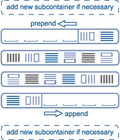
Figure 4–4: deque
The benefit of this design is that the data is mostly sequential in memory and access almost as fast as for vector [41]. At the same time, deque entries are never relocated. This doesn’t only save the cost of copy or move, it also allows us to store types that are neither copyable nor movable as we will show in the following.
![]() c++11/deque_emplace.cpp
c++11/deque_emplace.cpp
Pretty advanced: With the emplace methods, we can even create containers of non-copyable, non-movable classes. Say we have a solver class that contains neither copy nor move constructors (e.g., due to an atomic member; for atomic see §4.6):
![]()
struct parameters {};
struct solver
{
solver(const mat& ref, const parameters& para)
: ref(ref), para(para) {}
solver(const solver&) = delete;
solver(solver&&) = delete;
const mat& ref;
const parameters& para;
};
Several objects of this class are stored in a deque. Later, we iterate over those solvers:
void solve_x(const solver& s) { ... }
int main ()
{
parameters p1, p2, p3;
mat A, B, C;
deque<solver> solvers;
// solvers.push_back(solver(A, p1)); // would not compile
solvers.emplace_back(B, p1);
solvers.emplace_back(C, p2);
solvers.emplace_front(A, p1);
for (auto& s : solvers)
solve_x(s);
}
Please note that the solver class can only be used in container methods without data motion or copy. For instance, vector::emplace_back potentially copies or moves data and the corresponding code wouldn’t compile due to the deleted constructors in solver. Even with deque, we cannot use all member functions: insert and erase, for instance, need to move data. We must also use a reference for our loop variable s to avoid a copy there.
4.1.3.3 Lists
The list container (in <list>) is a doubly-linked list as shown in Figure 4–5 so that it can be traversed forward and backward (i.e., its iterators model BidirectionalIterator). In contrast to the preceding containers, we cannot access the n-th entry directly. An advantage overvector and deque is that insertion and deletion in the middle are less expensive.

Figure 4–5: Doubly-linked list (in theory)
List entries are never moved when others are inserted or deleted. Thus, only references and iterators of deleted entries are invalidated while all others keep their validity.
int main ()
{
list<int> l= {3, 4, 7, 9};
auto it= find(begin(l), end(l), 4), it2= find(begin(l), end(l), 7);
l.erase(it);
cout ![]() "it2 still points to "
"it2 still points to " ![]() *it2
*it2 ![]() '\n';
'\n';
}
The dynamic memory handling on each individual entry scatters them in the memory as illustrated in Figure 4–6 so that unfortunate cache behavior causes poorer performance than for vector and deque. Lists are more efficient for some operations but slower for many others so the overall performance is seldom better for list; compare, for instance, [28] or [52]. Fortunately, such performance bottlenecks can be quickly overcome in generically programmed applications by just changing the container types.
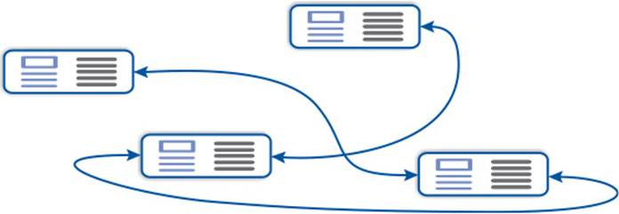
Figure 4–6: Doubly-linked list in practice
An entry of our list<int> takes 20 bytes on a typical 64-bit platform: two times 8 bytes for the 64-bit pointers and 4 bytes for int. When the backward iteration is not needed, we can save the space for one pointer and use a forward_list (in <forward_list>).
![]()
4.1.3.4 Sets and Multisets
The purpose of a set container is to store the information that a value belongs to the set. The entries in the set are internally sorted as a tree so that they can be accessed with logarithmic complexity. The presence of a value in a set can be tested by the member functions find and count.find returns an iterator referring to the value or if not found to the end iterator. If we don’t need the iterator, count is more convenient. In this case, it is more convenient to use count:
set<int> s= {1, 3, 4, 7, 9};
s.insert(5);
for (int i= 0; i < 6; ++i)
cout ![]() i
i ![]() " appears "
" appears " ![]() s.count(i)
s.count(i) ![]() " times.\n";
" times.\n";
yielding the expected output:
0 appears 0 time(s).
1 appears 1 time(s).
2 appears 0 time(s).
3 appears 1 time(s).
4 appears 1 time(s).
5 appears 1 time(s).
Multiple insertions of the same value have no impact; i.e., count always returns 0 or 1.
The container multiset additionally counts how often a value is inserted:
multiset<int> s= {1, 3, 4, 7, 9, 1, 1, 4};
s.insert(4);
for (int i= 0; i < 6; ++i)
cout ![]() i
i ![]() " appears "
" appears " ![]() s.count(i)
s.count(i) ![]() " time(s).\ n";
" time(s).\ n";
yielding:
0 appears 0 time(s).
1 appears 3 time(s).
2 appears 0 time(s).
3 appears 1 time(s).
4 appears 3 time(s).
5 appears 0 time(s).
For only checking whether a certain value is present in the multiset, find is more efficient as it doesn’t need to traverse replicated values.
Please note that there is no header file named multiset but the class multiset is also defined in <set>.
4.1.3.5 Maps and Multimaps
![]() c++11/map_test.cpp
c++11/map_test.cpp
A map is an associative container; i.e., values are associated with a Key. The key can have any type with an ordering: either provided by operator < (via the less functor) or by a functor establishing a strict weak ordering. The map provides a bracket operator for a concise access notation. The following program illustrates its usage:
map<string, double> constants=
{{"e", 2.7}, {"pi", 3.14}, {"h", 6.6e-34}};
cout ![]() "The Planck constant is "
"The Planck constant is " ![]() constants["h"]
constants["h"] ![]() '\n';
'\n';
constants["c"]= 299792458;
cout ![]() "The Coulomb constant is "
"The Coulomb constant is "
![]() constants["k"]
constants["k"] ![]() '\n'; // Access missing entry!
'\n'; // Access missing entry!
cout ![]() "The value of pi is "
"The value of pi is "
![]() constants.find("pi")->second
constants.find("pi")->second ![]() '\n';
'\n';
auto it_phi= constants.find("phi");
if (it_phi != constants.end())
cout ![]() "Golden ratio is "
"Golden ratio is " ![]() it_phi->second
it_phi->second ![]() '\n';
'\n';
cout ![]() "The Euler constant is"
"The Euler constant is"
![]() constants.at("e")
constants.at("e") ![]() "\n\n";
"\n\n";
for (auto& c : constants)
cout ![]() "The value of "
"The value of " ![]() c.first
c.first ![]() " is "
" is "
![]() c.second
c.second ![]() '\n';
'\n';
This yields:
The Planck constant is 6.6e-34
The Coulomb constant is 0
The circle's circumference pi is 3.14
The Euler constant is 2.7
The value of c is 2.99792e+08
The value of e is 2.7
The value of h is 6.6e-34
The value of k is 0
The value of pi is 3.14
The map is here initialized by a list of key-value pairs. Note that the value_type of the map is not double but pair<const string, double>. In the next two lines, we use the bracket operator for finding the value with key h and for inserting a new value for c. The bracket operator returns a reference to the value of that key. If the key is not found, a new entry is inserted with a default-constructed value. The reference to this value is then returned. In case of c, we assign a value to this reference and set up the key-value pair. Then we ask for the non-existing Coulomb constant and accidentally create an entry with a zero value.
To avoid inconsistencies between the mutable and the constant overload of [], the creators of STL omitted the constant overload altogether (a design choice we are not really happy with). To search keys in a constant map, we can use the classical method find or the C++11 method at.find is less elegant than [] but it saves us from accidentally inserting entries. It returns a const_iterator which refers to a key-value pair. If the key is not found, the end iterator is returned to which we should compare when the presence of the key is uncertain.
When we are sure that a key exists in the map, we can use at. It returns a reference to the value like []. The key difference is that an out_of_range exception is thrown when the the key is not found—even when the map is mutable. Thus, it cannot be used to insert new entries but provides a compact interface for finding entries.
When we iterate over the container, we get pairs of keys and associated values (as the values on their own would be meaningless).
![]() c++11/multimap_test.cpp
c++11/multimap_test.cpp
When a key can be associated with multiple values, we need a multimap. The entries with the same key are stored next to each other so we can iterate over them. The iterator range is provided by the methods lower_bound and upper_bound. In the next example we iterate over all entries with key equals 3 and print their values:
multimap<int, double> mm=
{{3, 1.3}, {2, 4.1}, {3, 1.8}, {4, 9.2}, {3, 1.5}};
for (auto it= mm.lower_bound(3),
end= mm.upper_bound(3); it != end; ++it)
cout ![]() "The value is "
"The value is " ![]() it->second
it->second ![]() '\n';
'\n';
This yields:
The value is 1.3
The value is 1.8
The value is 1.5
The last four containers—set, multiset, map, and multimap—are all realized as some kind of tree and have logarithmic complexity for the access. In the following section, we introduce containers with faster access regarding average complexity.
4.1.3.6 Hash Tables
![]()
![]() c++11/unordered_map_test.cpp
c++11/unordered_map_test.cpp
Hash tables are containers with very efficient search. In contrast to the preceding containers, hash maps have a constant complexity for a single access (when the hash function is reasonably good). To avoid name clashes with existing software, the standards committee refrained from names with “hash” and prepended “unordered” to the names of the ordered containers.
Unordered containers can be used in the same manner as their ordered counterparts:
unordered_map<string, double> constants=
{{"e", 2.7}, {"pi", 3.14}, {"h", 6.6e-34}};
cout ![]() "The Planck constant is "
"The Planck constant is " ![]() constants["h"]
constants["h"] ![]() '\n';
'\n';
constants["c"]= 299792458;
cout ![]() "The Euler constant is "
"The Euler constant is " ![]() constants.at("e")
constants.at("e") ![]() "\n\n";
"\n\n";
yielding the same results as map. If desired, a user-defined hash function can be provided.
Further reading: All containers provide a customizable allocator that allows us to implement our own memory management or to use platform-specific memory. The allocator interface is given, for instance, in [26], [43].
4.1.4 Algorithms
General-purpose STL algorithms are defined in the header <algorithm> and those primarily for number crunching in <numeric>.
4.1.4.1 Non-modifying Sequence Operations
find takes three arguments: two iterators that define the right-open interval of the search space, and a value to search for in that range. Each entry referred to by first is compared with value. When a match is found, the iterator pointing to it is returned; otherwise the iterator is incremented. If the value is not contained in the sequence, an iterator equal to last is returned. Thus, the caller can test whether the search was successful by comparing its result with last.
This is actually not a particularly difficult task and we could implement this by ourselves:
template <typename InputIterator, typename T>
InputIterator find(InputIterator first, InputIterator last,
const T& value)
{
while (first != last && *first != value)
++first;
return first;
}
This program snippet is indeed the standard way find is realized whereas specialized overloads for special iterators may exist.
![]() c++11/find_test.cpp
c++11/find_test.cpp
As a demonstration we consider a sequence of integer values containing the number 7 twice. We want to write the sub-sequence that starts with the first and ends with the second 7. In other words, we have to find the two occurrences and print out a closed interval—whereas STL always works on right-open intervals. This requires a little extra work:
vector<int> seq= {3, 4, 7, 9, 2, 5, 7, 8};
auto it= find(seq.begin(), seq.end(), 7); // first 7
auto end= find(it+1, seq.end(), 7); // second 7
for (auto past= end+1; it != past; ++it)
cout ![]() *it
*it ![]() ' ';
' ';
cout ![]() '\n';
'\n';
After we find the first 7, we restart the search from the succeeding position (so as not to find the same 7 again). In the for-loop, we increment the end iterator, so as not to include the second 7 in the printing. In the example above, we relied on the fact that 7 appears twice in the sequence. For robustness we throw user-defined exceptions when 7 isn’t found or is found only once.
To be more robust, we can check whether our search succeeded:
if (it == seq.end())
throw no_seven{};
...
if (end == seq.end())
throw one_seven{};
![]() c++11/find_test2.cpp
c++11/find_test2.cpp
The implementation above would not work for a list since we used the expressions it+1 and end+1. This requires that the iterators be random-access iterators. However, we can lift this requirement by copying one iterator and using an increment operation:
list<int> seq= {3, 4, 7, 9, 2, 5, 7, 8};
auto it= find(seq.begin(), seq.end(), 7), it2= it; // first 7
++it2;
auto end= find(it2, seq.end(), 7); // second 7
++end;
for (; it != end; ++it)
std::cout ![]() *it
*it ![]() ' ';
' ';
This iterator usage is not that different from the preceding implementation but it is more generic by avoiding the random-access operations. We can now use list, for instance. More formally: our second implementation only requires ForwardIterator for it and end while the first one needed RandomAccessIterator.
![]() c++11/find_test3.cpp
c++11/find_test3.cpp
In the same style, we can write a generic function to print the interval that works with all STL containers. Let’s go one step further: we also want to support classical arrays. Unfortunately, arrays have no member begin and end. (Right, they have no members at all.) C++11 donated them and all STL containers free functions named begin and end which allow us to be even more generic:
Listing 4–2: Generic function for printing a closed interval
struct value_not_found {};
struct value_not_found_twice {};
template <typename Range, typename Value>
void print_interval(const Range& r, const Value& v,
std::ostream& os= std::cout)
{
using std::begin; using std::end;
auto it= std::find(begin(r), end(r), v), it2= it;
if(it == end(r))
throw value_not_found();
++it2;
auto past= std::find(it2, end(r), v);
if (past == end(r))
throw value_not_found_twice();
++past;
for (; it != past; ++it)
os ![]() *it
*it ![]() ' ';
' ';
os ![]() '\n';
'\n';
}
int main ()
{
std::list<int> seq= {3, 4, 7, 9, 2, 5, 7, 8};
print_interval(seq, 7);
int array[]= {3, 4, 7, 9, 2, 5, 7, 8};
std::stringstream ss;
print_interval(array, 7, ss);
std::cout ![]() ss.str();
ss.str();
}
We also parameterized the output stream for not being restricted to std::cout. Please note the harmonic mixture of static and dynamic polymorphism in the function arguments: the types of the range r and the value v are instantiated during compilation while the output operator ![]() of osis selected at run time depending on the type that was actually referred to by os.
of osis selected at run time depending on the type that was actually referred to by os.
At this point, we want to draw your attention to the way we dealt with namespaces. When we use a lot of standard containers and algorithms, we can just declare
using namespace std;
directly after including the header files and don’t need to write std:: any longer. This works fine for small programs. In larger projects, we run sooner or later into name clashes. They can be laborious and annoying to fix (preventing is better than healing here). Therefore, we should import as little as possible—especially in header files. Our implementation of print_interval doesn’t rely on preceding name imports and can be safely placed in a header file. Even within the function, we don’t import the entire std namespace but limit ourselves to those functions that we really use.
Note that we did not qualify the namespace in some function calls, e.g., std::begin(r). This would work in the example above, but we would not cover user types that define a function begin in the namespace of the class. The combination of using std::begin andbegin(r) guarantees that std::begin is found. On the other hand, a begin function for a user type is found by ADL (§3.2.2) and would be a better match than std::begin. The same applies to end. In contrast, for the function find we didn’t want to call possible user overloads and made sure that it is taken from std.
find_if generalizes find by searching for the first entry that holds a general criterion. Instead of comparing with a single value it evaluates a Predicate—a function returning a bool. Say we search the first list entry larger than 4 and smaller than 7:
bool check(int i) { return i > 4 && i < 7; }
int main ()
{
list<int> seq= {3, 4, 7, 9, 2, 5, 7, 8};
auto it= find_if(begin(seq), end(seq), check);
cout ![]() "The first value in range is "
"The first value in range is " ![]() *it
*it ![]() '\n';
'\n';
}
Or we create the predicate in place:
![]()
auto it= find_if(begin(seq), end(seq),
[](int i){ return i > 4 && i < 7;} );
The searching and counting algorithms can be used similarly and the online manuals provide good documentation.
for_each: An STL function whose usefulness remains a mystery to us today is for_each. Its purpose is to apply a function on each element of a sequence. In C++03, we had to define a function object upfront or compose it with functors or pseudo-lambdas. A simple for-loop was easier to implement and much clearer to understand. Today we can create the function object on the fly with lambdas, but we also have a more concise range-based for-loop so the loop implementation is again simpler to write and to read. However, if you find for_each useful in some context, we do not want to discourage you. While for_each allows for modifying sequence elements according to the standard, it is still classified as non-mutable for historical reasons.
4.1.4.2 Modifying Sequence Operations
copy: The modifying operations have to be used with care because the modified sequence is usually only parameterized by the starting iterator. It is therefore our responsibility as programmers to make sure enough space is available. For instance, before we copy a container we canresize the target to the source’s size:
vector<int> seq= {3, 4, 7, 9, 2, 5, 7, 8}, v;
v.resize(seq.size());
copy(seq.begin(), seq.end(), v.begin ());
A nice demonstration of the iterators’ flexibility is printing a sequence by means of copy:
copy(seq.begin(), seq.end(), ostream_iterator<int>(cout, ", "));
The ostream_iterator builds a minimalistic iterator interface for an output stream: the ++ and * operations are void, comparison is not needed here, and an assignment of a value sends it to the referred output stream together with the delimiter.
unique is a function that is quite useful in numeric software: it removes the duplicated entries in a sequence. As a precondition the sequence must be sorted. Then unique can be used to rearrange the entries such that unique values are at the front and the replications at the end. An iterator to the first repeated entry is returned and can be used to remove the duplicates:
std::vector<int> seq= {3, 4, 7, 9, 2, 5, 7, 8, 3, 4, 3, 9};
sort(seq.begin(), seq.end());
auto it= unique(seq.begin(), seq.end());
seq.resize(distance(seq.begin(), it));
If this is a frequent task, we can encapsulate the preceding operations in a generic function parameterized with a sequence/range:
template <typename Seq>
void make_unique_sequence(Seq& seq)
{
using std::begin; using std::end; using std::distance;
std::sort(begin(seq), end(seq));
auto it= std::unique(begin(seq), end(seq));
seq.resize(distance(begin(seq), it));
}
There are many more mutating sequence operations that follow the same principles.
4.1.4.3 Sorting Operations
The sorting functions in the standard library are quite powerful and flexible and can be used in almost all situations. Earlier implementations were based on quick sort with O(n log n) average but quadratic worst-case complexity.2 Recent versions use intro-sort whose worst-case complexity isO(n log n), too. In short, there is very little reason to bother with our own implementation.
2. Lower worst-case complexity was already provided at that time by stable_sort and partial_sort.
By default, sort uses the < operator but we can customize the comparison, e.g., to sort sequences in descending order:
vector<int> seq= {3, 4, 7, 9, 2, 5, 7, 8, 3, 4, 3, 9};
sort(seq.begin(), seq.end(), [](int x, int y){return x > y;});
Lambdas come in handy again. Sequences of complex numbers cannot be sorted unless we define a comparison, for instance, by magnitude:
using cf= complex<float>;
vector<cf> v= {{3, 4}, {7, 9}, {2, 5}, {7, 8}};
sort(v.begin(), v.end(), [](cf x, cf y){return abs(x)<abs(y);});
Although not particularly meaningful here, a lexicographic order is also quickly defined with a lambda:
auto lex= [](cf x, cf y){return real(x)<real(y)
|| real(x)==real(y)&&imag(x)<imag(y);};
sort(v.begin(), v.end(), lex);
Many algorithms require a sorted sequence as a precondition as we have seen with unique. Set operations can also be performed on sorted sequences and do not necessarily need a set type.
4.1.4.4 Numeric Operation
The numeric operations from STL are found in header/library <numeric>. iota generates a sequence starting with a given value successively incremented by 1 for all following entries. accumulate evaluates by default the sum of a sequence and performs an arbitrary reduction when a binary function is provided by the user. inner_product performs by default a dot product whereby the general form allows for specifying a binary function object substituting the addition and multiplication respectively. partial_sum and adjacent_difference behave as their names suggest. The following little program shows all numeric functions at once:
vector<float> v= {3.1, 4.2, 7, 9.3, 2, 5, 7, 8, 3, 4},
w(10), x(10), y(10);
iota(w.begin(), w.end(), 12.1);
partial_sum(v.begin(), v.end(), x.begin());
adjacent_difference(v.begin(), v.end(), y.begin());
float alpha= inner_product(w.begin(), w.end(), v.begin(), 0.0f);
float sum_w= accumulate(w.begin(), w.end(), 0.0f),
product_w= accumulate(w.begin(), w.end(), 1.0f,
[](float x, float y){return x * y;});
The function iota was not part of C++03 but is integrated in the standard since C++11.
4.1.4.5 Complexity
Bjarne Stroustrup summarized the complexities of all STL algorithms in a concise table (Table 4–1) that we share with you.
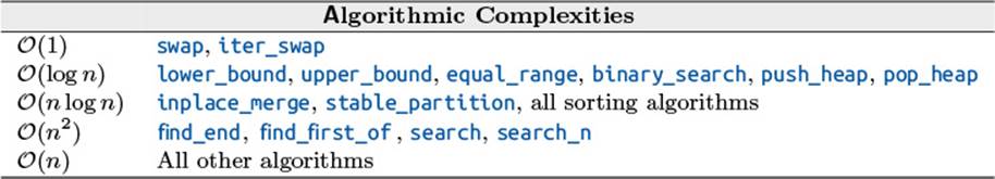
From [43, page 931]
Table 4–1: Complexity of STL Algorithms
4.1.5 Beyond Iterators
Iterators undoubtedly made an important contribution to modern programming in C++.
Nonetheless, they are quite dangerous and lead to inelegant interfaces.
Let’s start with the dangers. Iterators appear in pairs and only the programmer can assure that the two iterators used for the termination criterion really relate to each other. This offers us an unattractive repertoire of failures:
• The end iterator comes first.
• The iterators are from different containers.
• The iterator makes larger steps (over multiple entries) and doesn’t hit the end iterator.
In all these cases, the iteration can run over arbitrary memory and might only stop when the program leaves the accessible address space. A program crash is probably still our best option because we see where we failed. An execution that at some point stops the iteration has most likely already ruined a lot of data so the program can cause serious damage before ending in a crash or in an alleged success.
Similarly, STL functions on multiple containers only take a pair of iterators from one container3 and solely the beginning iterator from the other containers, e.g.:
3. A pair of iterators does not necessarily represent an entire container. It can also refer to a part of a container or some more general abstraction. Considering entire containers only is already enough to demonstrate catastrophic consequences of even little errors.
copy(v.begin(), v.end(), w.begin());
Thus, it cannot be tested whether the target of the copy provides enough space and random memory can be overwritten.
Finally, the interface of iterator-based functions is not always elegant. Consider
x= inner_product(v.begin(), v.end(), w.begin());
versus
x= dot(v, w);
The example speaks for itself. Plus, the second notion allows us to check that v and w match in size.
C++ 17 may introduce Ranges. These are all types providing a begin and an end function which return iterators. This includes all containers but is not limited to it. A range can also represent a sub-container, the reverse traversal of a container, or some transformed view. The ranges will trim the function interface nicely and will also allow size checks.
In the meantime, we do ourselves a favor by adding functions on top of those with an iterator interface. There is nothing wrong with using iterator-based functions on low or intermediate levels. They are excellent to provide the most general applicability. But in most cases we don’t need this generality because we operate on complete containers, and size-checking functions with a concise interface allow us to write more elegant and more reliable applications. On the other hand, existing iterator-based functions can be called internally as we did for print_interval inListing 4–2. Likewise, we could realize a concise dot function from inner_product. Thus:
Iterator-Based Functions
If you write iterator-based functions, provide a user-friendly interface on top of them.
Final remark: This section only scratches the surface of STL and is intended as a mere appetizer.
4.2 Numerics
In this section we illustrate how the complex numbers and the random-number generators of C++ can be used. The header <cmath> contains a fair number of numeric functions whose usage is straightforward, not needing further illustration.
4.2.1 Complex Numbers
We already demonstrated how to implement a non-templated complex class in Chapter 2 and used the complex class template in Chapter 3. To not repeat the obvious again and again, we illustrate the usage with a graphical example.
4.2.1.1 Mandelbrot Set
The Mandelbrot set—named after its creator, Benoît B. Mandelbrot—is the set of complex numbers that don’t reach infinity by successive squaring and adding the original value:
![]()
where
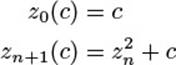
It can be shown that a point is outside the Mandelbrot set when |zn(c)| > 2. The most expensive part of computing the magnitude is the square root at the end. C++ provides a function norm which is the square of abs, i.e., the calculation of abs without the final sqrt. Thus, we replace the continuation criterion abs(z) <= 2 with norm(z) <= 4.
![]() c++11/mandelbrot.cpp
c++11/mandelbrot.cpp
The visualization of the Mandelbrot set is a color coding of the iterations needed to reach that limit. To draw the fractal, we used the cross-platform library Simple DirectMedia Layer (SDL 1.2). The numeric part is realized by the class mandel_pixel that computes for each pixel on the screen how many iterations are needed until norm(z) > 4 and which color that represents:
class mandel_pixel
{
public:
mandel_pixel(SDL_Surface* screen, int x, int y,
int xdim, int ydim, int max_iter)
: screen(screen), max_iter(max_iter), iter(0), c(x, y)
{
// scale y to [-1.2,1.2] and shift -0.5+0i to the center
c*= 2.4f / static_cast<float>(ydim);
c-= complex<float>(1.2 * xdim / ydim + 0.5, 1.2);
iterate ();
}
int iterations() const { return iter; }
uint32_t color() const { ... }
private:
void iterate()
{
complex<float> z= c;
for (; iter < max_iter && norm(z) <= 4.0f; iter++)
z= z * z + c;
};
// ...
int iter;
complex <float> c;
};
The complex numbers are scaled such that their imaginary parts lie between -1.2 and 1.2 and are shifted by 0.5 to the left. We have omitted the code lines for the graphics, as they are beyond the scope of this book. The complete program is found on GitHub, and the resulting picture in Figure 4–7.

Figure 4–7: Mandelbrot set
In the end, our core computation is realized in three lines and the other ≈ 50 lines are needed to draw a nice picture, despite our having chosen a very simple graphics library. This is unfortunately not an uncommon situation: many real-world applications contain far more code for file I/O, database access, graphics, web interfaces, etc., than for the scientific core functionality.
4.2.1.2 Mixed Complex Calculations
As demonstrated before, complex numbers can be built from most numeric types. In this regard, the library is quite generic. For its operations it is not so generic: a value of type complex<T> can only be added (subtracted, etc.) with a value of type complex<T> or T. As a consequence, the simple code
complex<double> z(3, 5), c= 2 * z;
doesn’t compile since no multiplication is defined for int and complex<double>. The problem is easily fixed by replacing 2 with 2.0. However, the issue is more annoying in generic functions, e.g.:
template <typename T>
inline T twice(const T& z)
{ return 2 * z; }
int main ()
{
complex<double> z(3, 5), c;
c= twice (z);
}
The function twice will not compile for the same reason as before. If we wrote 2.0 * z it would compile for complex<double> but not for complex<float> or complex<long double>. The function
template <typename T>
complex<T> twice(const complex<T>& z)
{ return T{2} * z; }
works with all complex types—but only with complex types. In contrast, the following:
template <typename T>
inline T twice(const T& z)
{ return T{2} * z; }
compiles with complex and non-complex types. However, when T is a complex type, 2 is unnecessarily converted into a complex and four multiplications plus two additions are performed where only half of them are needed. A possible solution is to overload the last two implementations. Alternatively, we can write type traits to deal with it.
The programming becomes more challenging when multiple arguments of different types are involved, some of them possibly complex numbers. The Matrix Template Library (MTL4, Section 4.7.3) provides mixed arithmetic for complex numbers. We are committed to incorporate this feature into future standards.
4.2.2 Random Number Generators
![]()
Many application domains—like computer simulation, game programming, or cryptography—use random numbers. Every serious programming language thus offers generators for them. Such generators produce sequences of numbers that appear random. A random generator may depend on physical processes like quantum phenomena. However, most generators are based on pseudo-random calculations. They have an internal state—called a Seed—that is transformed by deterministic computation each time a pseudo-random number is requested. Thus, a pseudo-random number generator (PRNG) always emits the same sequence when started with the same seed.
Before C++11, there were only the rand and srand functions from C with very limited functionality. More problematic is that there are no guarantees for the quality of generated numbers and it is indeed quite low on some platforms. Therefore, a high-quality <random> library was added in C++11. It was even considered to deprecate rand and srand altogether in C++. They are still around but should really be avoided where the quality of random numbers is important.
4.2.2.1 Keep It Simple
The random number generators in C++11 provide a lot of flexibility which is very useful for experts but somewhat overwhelming for beginners. Walter Brown proposed a set of novice-friendly functions [6]. Slightly adapted,4 they are:
4. Walter used return type deduction of non-lambda functions which is only available in C++14 and higher. We further shortened the function name from pick_a_number to pick.
#include <random>
std::default_random_engine& global_urng()
{
static std::default_random_engine u{};
return u;
}
void randomize()
{
static std::random_device rd{};
global_urng().seed(rd());
}
int pick (int from, int thru)
{
static std::uniform_int_distribution<> d{};
using parm_t= decltype(d)::param_type;
return d(global_urng(), parm_t{from, thru});
}
double pick(double from, double upto)
{
static std::uniform_real_distribution <> d{};
using parm_t= decltype(d)::param_type;
return d(global_urng(), parm_t{from, upto});
}
To start with random numbers, you could just copy these three function into the project and look at the details later. Walter’s interface is pretty simple and nonetheless sufficient for many practical purposes like code testing. We only need to remember the following three functions:
• randomize: Make the following numbers really random by initializing the generator’s seed.
• pick(int a, int b): Give me an int in the interval [a, b] when a and b are int.
• pick(double a, double b): Give me an double in the right-open interval [a, b) when a and b are double.
Without calling randomize, the sequence of generated numbers is equal each time which is desirable in certain situations: finding bugs is much easier with reproducible behavior. Note that pick includes the upper bound for int but not for double to be consistent with standard functions. global_urng can be considered as an implementation detail for the moment.
With those functions, we can easily write loops for rolling dice:
randomize();
cout ![]() "Now, we roll dice:\n";
"Now, we roll dice:\n";
for (int i= 0; i < 15; ++i)
cout ![]() pick(1, 6)
pick(1, 6) ![]() endl;
endl;
cout ![]() "\nLet's roll continuous dice now: ;-)\n";
"\nLet's roll continuous dice now: ;-)\n";
for (int i= 0; i < 15; ++i)
cout ![]() pick(1.0, 6.0)
pick(1.0, 6.0) ![]() endl;
endl;
In fact, this is even simpler than the old C interface. Apparently it is too late for C++14, but the author would be glad to see these functions in future standards. In the following section, we will use this interface for testing.
4.2.2.2 Randomized Testing
![]() c++11/random_testing.cpp
c++11/random_testing.cpp
Say we want to test whether our complex implementation from Chapter 2 is distributive:
![]()
The multiplication is canonically implemented as
inline complex operator*(const complex& c1, const complex& c2)
{
return complex(real(c1) * real(c2) - imag(c1) * imag(c2),
real(c1) * imag(c2) + imag(c1) * real(c2));
}
To cope with rounding errors we introduce a function similar that checks relative difference:
#include <limits>
const double eps= 10 * numeric_limits<double>::epsilon();
inline bool similar(complex x, complex y)
{
double sum= abs(x) + abs(y);
if (sum < 1000 * numeric_limits<double>::min())
return true;
return abs(x - y) / sum <= eps;
}
To avoid divisions by zero we treat two complex numbers as similar if their magnitudes are both very close to zero (the sum of magnitudes smaller than 1000 times the minimal value representable as double). Otherwise, we relate the difference of the two values to the sum of their magnitudes. This should not be larger than 10 times epsilon, the difference between 1 and the next value representable as double. This information is provided by the <limits> library later introduced in Section 4.3.1.
Next, we need a test that takes a triplet of complex numbers for the variables in (4.1) and that checks the similarity of the terms on both sides thereafter:
struct distributivity_violated {};
inline void test(complex a, complex b, complex c)
{
if (!similar(a * (b + c), a * b + a * c)) {
cerr ![]() "Test detected that "
"Test detected that " ![]() a
a ![]() ...
...
throw distributivity_violated();
}
}
If a violation is detected, the critical values are reported on the error stream and a user-defined exception is thrown. Finally, we implement the random generation of complex numbers and the loops over test sets:
const double from= -10.0, upto= 10.0;
inline complex mypick()
{ return complex(pick(from, upto), pick(from, upto)); }
int main ()
{
const int max_test= 20;
randomize();
for (int i= 0; i < max_test; ++i) {
complex a= mypick();
for (int j= 0; j < max_test; j++) {
complex b= mypick();
for (int k= 0; k < max_test; k++) {
complex c= mypick();
test (a, b, c);
}
}
}
}
Here we only tested with random numbers from [–10, 10) for the real and the imaginary parts; whether this is sufficient to reach good confidence in the correctness is left open. In large projects it definitely pays off to build a reusable test framework. The pattern of nested loops containing random value generation and a test function in the innermost loop is applicable in many situations. It could be encapsulated in a class which might be variadic to handle properties involving different numbers of variables. The generation of a random value could also be provided by a special constructor (e.g., marked by a tag), or a sequence could be generated upfront. Different approaches are imaginable. The loop pattern in this section was chosen for the sake of simplicity.
To see that the distributivity doesn’t hold precisely, we can decrease eps to 0. Then, we see an (abbreviated) error message like
Test detected that (-6.21,7.09) * ((2.52,-3.58) + (-4.51,3.91))
!= (-6.21,7.09) * (2.52,-3.58) + (-6.21,7.09) * (-4.51,3.91)
terminate called after throwing 'distributivity_violated'
Now we go into the details of random number generation.
4.2.2.3 Engines
The library <random> contains two kinds of functional objects: generators and distributions. The former generate sequences of unsigned integers (the precise type is provided by each class’s typedef). Every value should have approximately the same probability. The distribution classes map these numbers to values whose probability corresponds to the parameterized distribution.
Unless we have special needs, we can just use the default_random_engine. We have to keep in mind that the random number sequence depends deterministically on its seed and that each engine is initialized with the same seed whenever an object is created. Thus, a new engine of a given type always produces the same sequence, for instance:
void random_numbers()
{
default_random_engine re;
cout ![]() "Random numbers: ";
"Random numbers: ";
for (int i= 0; i < 4; i++)
cout ![]() re
re ![]() (i < 3 ? ", " : "");
(i < 3 ? ", " : "");
cout ![]() '\n';
'\n';
}
int main ()
{
random_numbers();
random_numbers();
}
yielded on the author’s machine:
Random numbers: 16807, 282475249, 1622650073, 984943658
Random numbers: 16807, 282475249, 1622650073, 984943658
To get a different sequence in each call of random_numbers, we have to create a persistent engine by declaring it static:
void random_numbers()
{
static default_random_engine re;
...
}
Still, we have the same sequence in every program run. To overcome this, we must set the seed to an almost truly random value. Such a value is provided by random_device:
void random_numbers()
{
static random_device rd;
static default_random_engine re(rd());
...
}
random_device returns a value that depends on measurements of hardware and operating system events and can be considered virtually random (i.e., a very high Entropy is achieved). In fact, random_device provides the same interface as an engine except that the seed cannot be set. So, it can be used to generate random values as well, at least when performance doesn’t matter. On our test machine, it took 4–13 ms to generate a million random numbers with the default_random_engine and 810–820 ms with random_device. In applications that depend on high-quality random numbers, like in cryptography, the performance penalty can still be acceptable. In most cases, it should suffice to generate only the starting seed with random_device.
Among the generators there are primary engines, parameterizable adapters thereof, and predefined adapted engines:
• Basic engines that generate random values:
– linear_congruential_engine,
– mersenne_twister_engine, and
– subtract_with_carry_engine.
• Engine adapters to create a new engine from another one:
– discard_block_engine: ignores n entries from the underlying engine each time;
– independent_bits_engine: map the primary random number to w bits;
– shuffle_order_engine: modifies the order of random numbers by keeping an internal buffer of the last values.
• Predefined adapted engines build from basic engines by instantiation or adaption:
– knuth_b
– minstd_rand
– minstd_rand0
– mt19937
– mt19937_64
– ranlux24
– ranlux24_base
– ranlux48
– ranlux48_base
The predefined engines in the last group are just type definitions, for instance:
typedef shuffle_order_engine <minstd_rand0,256> knuth_b;
4.2.2.4 Distribution Overview
As mentioned before, the distribution classes map the unsigned integers to the parameterized distributions. Table 4–2 summarizes the distributions defined in C++11. Due to space limits, we used some abbreviated notations. The result type of a distribution can be specified as an argument of the class template where I represents an integer and R a real type. When different symbols are used in the constructor (e.g., m) and the describing formula (e.g., μ), we denoted the equivalence in the precondition (like m ≡ μ). For consistency’s sake, we used the same notation in the log-normal and the normal distribution (in contrast to other books, online references, and the standard).
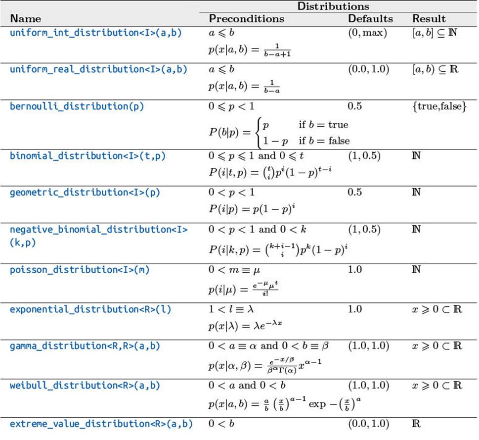
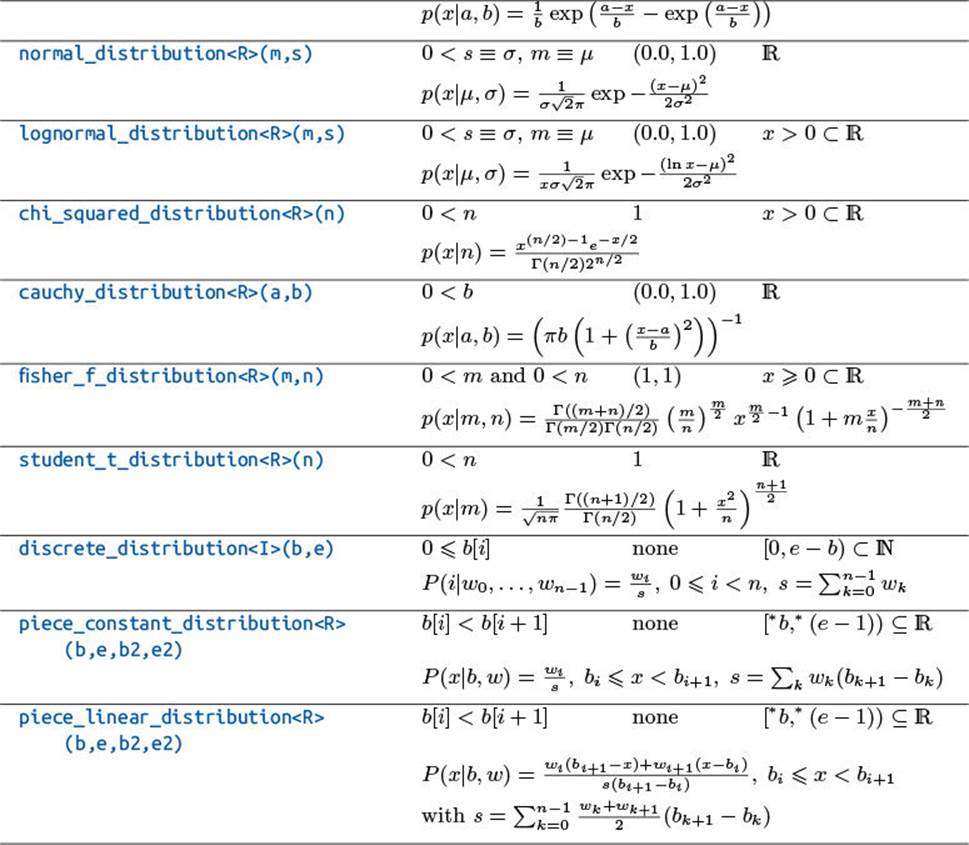
Table 4–2: Distribution Overview
4.2.2.5 Using a Distribution
Distributions are parameterized with a random number generator, for instance:
default_random_engine re(random_device{}());
normal_distribution<> normal;
for (int i= 0; i < 6; ++i)
cout ![]() normal(re)
normal(re) ![]() endl;
endl;
Here we created an engine—randomized in the constructor—and a normal distribution of type double with default parameters μ = 0.0 and σ = 1.0. In each call of the distribution-based generator, we pass the random engine as an argument. The following is an example of the program’s output:
-0.339502
0.766392
-0.891504
0.218919
2.12442
-1.56393
It will of course be different each time we call it.
Alternatively, we can use the bind function from the <functional> header (§4.4.2) to bind the distribution to the engine:
auto normal= bind(normal_distribution<>{},
default_random_engine(random_device{}()));
for (int i= 0; i < 6; ++i)
cout ![]() normal()
normal() ![]() endl;
endl;
The function object normal can now be called without arguments. In this situation, bind is more compact than a lambda—even with init capture (§3.9.4):
![]()
auto normal= [re= default_random_engine(random_device{}()),
n= normal_distribution<>{}]() mutable
{ return n(re); };
In most other scenarios, lambdas lead to more readable program sources than bind but the latter seems more suitable for binding random engines to distributions.
4.2.2.6 Stochastic Simulation of Share Price Evolution
With the normal distribution we can simulate possible developments of a stock’s share price in the Black-Scholes model by Fischer Black and Myron Scholes. The mathematical background is for instance discussed in Jan Rudl’s lecture [36, pages 94–95] (in German, unfortunately) and in other quantitative finance publications like [54]. Starting with an initial price of ![]() with an expected yield of μ, a variation of σ, a normally distributed random value Zi, and a time step Δ, the share price at t = i · Δ is simulated with respect to the preceding time step by
with an expected yield of μ, a variation of σ, a normally distributed random value Zi, and a time step Δ, the share price at t = i · Δ is simulated with respect to the preceding time step by
![]()
Subsuming ![]() and
and ![]() , the equation simplifies to
, the equation simplifies to
![]()
![]() c++11/black_scholes.cpp
c++11/black_scholes.cpp
The development of S1 with the parameters μ = 0.05, σ = 0.3, Δ = 1.0, t = 20 as constants according to (4.2) can now be programmed in a few lines:
default_random_engine re(random_device{}());
normal_distribution<> normal;
const double mu= 0.05, sigma= 0.3, delta= 0.5, years= 20.01,
a= sigma * sqrt(delta),
b= delta * (mu - 0.5 * sigma * sigma);
vector<double> s= {345.2}; // Start with initial price
for (double t= 0.0; t < years; t+= delta)
s.push_back( s.back() * exp(a * normal(re) + b) )
Figure 4–8 depicts five possible developments of the share price for the parameters from the previous code.

Figure 4–8: Simulated share price over 20 years
We hope that this introduction to random numbers will give you a smooth start to the exploration of this powerful library.
4.3 Meta-programming
In this section, we will give you a foretaste of meta-programming. Here, we will focus on the library support and in Chapter 5 we will provide more background.
4.3.1 Limits
A very useful library for generic programming is <limits> which provides important information on types. It can also prevent surprising behavior when the source is compiled on another platform and some types are implemented differently. The header <limits> contains the class template numeric_limits that delivers type-specific information on intrinsic types. This is especially important when dealing with numeric type parameters.
In Section 1.7.5, we demonstrated that only some digits of floating-point numbers are written to the output. Especially when the numbers are written to files, we want to be able to read back the correct value. The number of decimal digits is given in numeric_limits as a compile-time constant. The following program prints 1/3 in different floating-point formats with one extra digit:
#include <iostream>
#include <limits>
using namespace std;
template <typename T>
inline void test(const T& x)
{
cout ![]() "x = "
"x = " ![]() x
x ![]() " (";
" (";
int oldp= cout.precision(numeric_limits<T>::digits10 + 1);
cout ![]() x
x ![]() ")"
")" ![]() endl;
endl;
cout.precision(oldp);
}
int main ()
{
test(1.f/3.f);
test(1./3.0);
test(1./3.0l);
}
This yields
x = 0.333333 (0.3333333)
x = 0.333333 (0.3333333333333333)
x = 0.333333 (0.3333333333333333333)
Another example is computing the minimum value of a container. When the container is empty we want the identity element of the minimum operation, which is the maximal representable value of the corresponding type:
template <typename Container>
typename Container::value_type
inline minimum(const Container& c)
{
using vt= typename Container::value_type;
vt min_value= numeric_limits<vt>::max();
for (const vt& x : c)
if (x < min_value)
min_value= x;
return min_value;
}
The method max is static and can be called for the type directly without the need of an object. Likewise, the static method min yields the minimal value—more precisely the minimal representable value for int types and the minimal value larger than 0 for floating-point types. Therefore, C++11 introduces the member lowest which yields the smallest value for all fundamental types.
![]()
Termination criteria in fixed-point computations should be type-dependent. When they are too large, the result is unnecessarily imprecise. When they are too small, the algorithm might not terminate (i.e., it may only finish when two consecutive values are identical). For a floating-point type, the static method epsilon yields the smallest value to be added to 1 for a number larger than 1, in other words, the smallest possible increment (with respect to 1), also called Unit of Least Precision (ULP). We already used it in Section 4.2.2.2 for determining the similarity of two values.
The following generic example computes the square root iteratively. The termination criterion is that the approximated result of ![]() should be in an
should be in an ![]() -environment of x. To ascertain that our environment is large enough, we scale it with x and double it afterward:
-environment of x. To ascertain that our environment is large enough, we scale it with x and double it afterward:
template <typename T>
T square_root(const T& x)
{
const T my_eps= T{2} * x * numeric_limits<T>::epsilon();
T r= x;
while (std::abs((r * r) - x) > my_eps)
r= (r + x/r) / T{2};
return r;
}
The complete set of numeric_limits’s members is available in online references like www.cppreference.com or www.cplusplus.com.
4.3.2 Type Traits
![]()
![]() c++11/type_traits_example.cpp
c++11/type_traits_example.cpp
The type traits that many programmers have already used for several years from the Boost library were standardized in C++11 and provided in <type_traits>. We refrain at this point from enumerating them completely and refer you instead to the before-mentioned online manuals. Some of the type traits—like is_const (§5.2.3.3)—are very easy to implement by partial template specialization. Establishing domain-specific type traits in this style (e.g., is_matrix) is not difficult and can be quite useful. Other type traits that reflect the existence of functions or properties thereof—such as is_nothrow_assignable—are quite tricky to implement. Providing type traits of this kind requires a fair amount of expertise (if not black magic).
![]() c++11/is_pod_test.cpp
c++11/is_pod_test.cpp
With all the new features, C++11 did not forget its roots. There are type traits that allow us to check the compatibility with C. is_pod tells us whether a type is a Plain Old Data type (POD). These are all intrinsic types and “simple” classes that can be used in a C program. In case we need a class that is used in C and C++ programs, it is best to define it only once in a C-compatible fashion: as struct and with no or conditionally compiled methods. It should not contain virtual functions and static data members. In sum, the memory layout of the class must be compatible with C and the default and copy constructor must be Trivial: they are either declared as default or compiler-generated in a default manner. For instance, the following class is POD:
struct simple_point
{
# ifdef __cplusplus
simple_point(double x, double y) : x(x), y(y) {}
simple_point() = default;
simple_point(initializer_list<double> il)
{
auto it= begin(il);
x= *it;
y= *next(it);
}
# endif
double x, y;
};
We can check this as follows:
cout ![]() "simple_point is pod = "
"simple_point is pod = " ![]() boolalpha
boolalpha
![]() is_pod<simple_point>::value
is_pod<simple_point>::value ![]() endl;
endl;
All C++-only code is conditionally compiled: the macro __cplusplus is predefined in all C++ compilers. Its value reveals which standard the compiler supports (in the current translation). The class above can be used with an initializer list:
simple_point p1= {3.0, 7.0};
and is nonetheless compilable with a C compiler (unless some clown defined __cplusplus in the C code). The CUDA library implements some classes in this style. However, such hybrid constructs should only be used when really necessary to avoid surplus maintenance effort and inconsistency risks.
![]() c++11/memcpy_test.cpp
c++11/memcpy_test.cpp
Plain old data is stored contiguously in memory and can be copied as raw data without calling a copy constructor. This is achieved with the traditional functions memcpy or memmove. However, as responsible programmers we check upfront with is_trivially_copyable whether we can really call these low-level copy functions:
simple_point p1{3.0, 7.1}, p2;
static_assert(std::is_trivially_copyable<simple_point>::value,
"simple_point is not as simple as you think "
"and cannot be memcpyd!");
std::memcpy(&p2, &p1, sizeof(p1));
Unfortunately, the type trait was implemented late in several compilers. For instance, g++ 4.9 and clang 3.4 don’t provide it while g++ 5.1 and clang 3.5 do.
This old-style copy function should only be used in the interaction with C. Within pure C++ programs it is better to rely on STL copy:
copy(&x, &x + 1, &y);
This works regardless of our class’s memory layout and the implementation of copy uses memmove internally when the types allow for it.
C++14 adds some template aliases like
![]()
conditional_t<B, T, F>
as a shortcut for
typename conditional<B, T, F>::type
Likewise, enable_if_t is an abbreviation for the type of enable_if.
4.4 Utilities
![]()
C++11 adds new libraries that make modern programming style easier and more elegant. For instance, we can return multiple results more easily, refer to functions and functors more flexibly, and create containers of references.
4.4.1 Tuple
![]()
When a function computes multiple results, they used to be passed as mutable reference arguments. Assume we implement an LU factorization with pivoting taking a matrix A and returning the factorized matrix LU and the permutation vector p:
void lu(const matrix& A, matrix& LU, vector& p) { ... }
We could also return either LU or p as function results and pass the other object by reference. This mixed approach is even more confusing.
![]() c++11/tuple_move_test.cpp
c++11/tuple_move_test.cpp
To return multiple results without implementing a new class, we can bundle them into a Tuple. A tuple (from <tuple>) differs from a container by allowing different types. In contrast to most containers, the number of objects must be known at compile time. With a tuple we can return both results of our LU factorization at once:
tuple<matrix, vector> lu(const matrix& A)
{
matrix LU(A);
vector p(n);
// ... some computations
return tuple<matrix, vector>(LU, p);
}
The return statement can be simplified with the helper function make_tuple deducing the type parameters:
tuple<matrix, vector> lu(const matrix& A)
{
...
return make_tuple(LU, p);
}
make_tuple is especially convenient in combination with auto variables:
auto t= make_tuple(LU, p, 7.3, 9, LU*p, 2.0+9.0i);
The caller of our function lu will probably extract the matrix and the vector from the tuple with the function get:
tuple<matrix, vector> t= lu(A);
matrix LU= get<0>(t);
vector p= get<1>(t);
Here, all types can be deduced as well:
auto t= lu(A);
auto LU= get<0>(t);
auto p= get<1>(t);
The function get takes two arguments: a tuple and a position therein. The latter is a compile-time parameter. Otherwise the type of the result would not be known. If the index is too large, the error is detected during compilation:
auto t= lu(A);
auto am_i_stupid= get<2>(t); // Error during compilation
In C++14, the tuple entries can also be accessed by their type if this is unambiguous:
![]()
auto t= lu(A);
auto LU= get<matrix>(t);
auto p= get<vector>(t);
Then we are not obliged any longer to memorize the internal order in the tuple. Alternatively, we can use the function tie to separate the entries in the tuple. This is often more elegant. In this case, we have to declare compatible variables beforehand:
matrix LU;
vector p;
tie(LU, p)= lu(A);
tie looks quite mysterious at first but its implementation is surprisingly simple: it creates an object with references to function arguments. Assigning a tuple to that object performs assignments of each tuple member to the respective reference.
The implementation with tie has a performance advantage over the implementation with get. When we pass the result of function lu directly to tie, it is still an rvalue (it has no name) and we can move the entries. With an intermediate variable, it becomes an lvalue (it has a name) and the entries must be copied. To avoid the copies, we can also move the tuple entries explicitly:
auto t= lu(A);
auto LU= get<0>(move(t));
auto p= get<1>(move(t));
Here, we step on rather thin ice. In principle, an object is considered expired after move is applied on it. It is allowed to be in any state as long as the destructor doesn’t crash. In our example, we read t again after using move upon it. This is correct in this special situation. move turns t into an rvalue and we can do whatever we want to its data. But we don’t. When LU is created, we only take the data of the tuple’s entry 0 and don’t touch entry 1. Conversely, we only steal the data from t’s entry 1 in p’s creation and don’t access the expired data in entry 0. Thus, the two operations move entirely disjoint data. Nonetheless, multiple occurrences of move on the same data item are very dangerous and must be analyzed carefully (like we did).
After discussing the efficient data handling on the caller side, we should take another look at the function lu. The resulting matrix and vector are copied into the tuple when returned from the function. Within a return statement it is safe to move all data from the function5 as it is going to be destroyed anyway. Here is the revised function excerpt:
5. Unless an object appears twice in the tuple.
tuple<matrix, vector> lu(const matrix& A)
{
...
return make_tuple(move(LU), move(p));
}
Now that we have avoided all copies, the implementation returning a tuple is as efficient as the code with mutable references, at least when the result is used to initialize variables. When the result is assigned to existing variables, we still have the overhead of allocating and releasing memory.
The other heterogeneous class in C++ is pair. It already existed in C++03 and still does. pair is equivalent to a tuple with two arguments. Conversions from one to another exist so pair and two-argument tuple can be exchanged with each other and even mixed. The examples in this section could all be implemented with pair. Instead of get<0>(t) we could also write t. first (and t.second for get<1>(t)).
![]() c++11/boost_fusion_example.cpp
c++11/boost_fusion_example.cpp
Further reading: The library Boost::Fusion is designed for fusing meta-programming with classical (run-time) programming. Using this library, we can write code that iterates over tuples. The following program implements a generic functor printer that is called for each entry of tuple t:
struct printer
{
template <typename T>
void operator()(const T& x) const
{ std::cout ![]() "Entry is "
"Entry is " ![]() x
x ![]() std::endl; }
std::endl; }
};
int main ()
{
auto t= std::make_tuple(3, 7u, "Hallo", std::string("Hi"),
std::complex<float>(3, 7));
boost::fusion::for_each(t, printer{});
}
The library further offers more powerful features for traversing and transforming heterogeneous type composites (boost::fusion::for_each is in our opinion way more useful than std::for_each). Especially when functionality at compile and run time interferes in non-trivial fashion, Boost Fusion is indispensable.
The widest functionality in the area of meta-programming is supplied by the Boost Meta-Programming Library (MPL) [22]. The library implements most of the STL algorithms (§4.1) and also provides similar data types: for instance, vector and map are realized as compile-time containers. Especially, the combination of MPL and Boost Fusion is extremely powerful when functionality at compile and run time interferes in a non-trivial fashion. A new library at the time of this writing is Hana [11] which addresses compile- and run-time calculations with a more functional approach. It leads to significantly more compact programs while heavily relying on C++14 features.
4.4.2 function
![]()
![]() c++11/function_example.cpp
c++11/function_example.cpp
The function class template in <functional> is a generalized function pointer. The function type specification is passed as a template argument like this:
double add(double x, double y)
{ return x + y; }
int main ()
{
using bin_fun= function<double(double, double)>;
bin_fun f= &add;
cout ![]() "f(6, 3) = "
"f(6, 3) = " ![]() f(6, 3)
f(6, 3) ![]() endl;
endl;
}
The function wrapper can hold functional entities of different kinds with the same return type and the same list of parameter types.6 We can even build containers of compatible functional objects:
6. Thus, they may have different signatures since equal function names aren’t required. In contrast, the equality of signatures doesn’t impose the same return types.
vector<bin_fun> functions;
functions.push_back(&add);
When a function is passed as an argument, its address is taken automatically. Just as arrays are implicitly decayed to pointers, functions are decayed to pointer pointers. So, we can omit the address operator &:
functions.push_back(add);
When a function is declared inline, its code should be inserted in the calling context. Nonetheless, each inline function gets a unique address when needed which can be stored as a function object as well:
inline double sub(double x, double y)
{ return x - y; }
functions.push_back(sub);
Again, the address is taken implicitly. Functors can be stored as well:
struct mult {
double operator()(double x, double y) const { return x * y; }
};
functions.push_back(mult{});
Here we constructed an anonymous object with the default constructor. Class templates are not types so we cannot create objects thereof:
template <typename Value>
struct power {
Value operator()(Value x, Value y) const { return pow(x, y); }
};
functions.push_back(power()); // Error
We can only construct objects from instantiated templates:
functions.push_back(power<double>{});
On the other hand, we can create objects from classes that contain function templates:
struct greater_t {
template <typename Value>
Value operator()(Value x, Value y) const { return x > y; }
} greater_than;
functions.push_back(greater_than);
In this context, the template call operator must be instantiatable for function type. As a counter-example, the following statement doesn’t compile as we cannot instantiate it to a function with different argument types:
function<double(float, double)> ff= greater_than; // Error
Last but not least, lambdas with matching return and argument types can be stored as function objects:
functions.push_back([](double x, double y){ return x / y; });
Each entry of our container can be called like a function:
for (auto& f : functions)
cout ![]() "f(6, 3) = "
"f(6, 3) = " ![]() f(6, 3)
f(6, 3) ![]() endl;
endl;
yielding the expected output:
f(6, 3) = 9
f(6, 3) = 3
f(6, 3) = 18
f(6, 3) = 216
f(6, 3) = 1
f(6, 3) = 2
Needless to say, this function wrapper is preferable to function pointers in terms of flexibility and clarity (which we pay for with some overhead).
4.4.3 Reference Wrapper
![]()
![]() c++11/ref_example.cpp
c++11/ref_example.cpp
Assume we want to create a list of vectors or matrices—possibly large ones. In addition, suppose that some entries appear multiple times. Therefore, we don’t want to store the actual vectors or matrices. We could create a container of pointers, but we want to avoid all the danger related to them (§1.8.2).
Unfortunately, we cannot create a container of references:
vector<vector<int>&> vv; // Error
C++11 provides for this purpose a reference-like type called reference_wrapper that can be included with the header <functional>:
vector<reference_wrapper<vector<int> > > vv;
The vectors can be inserted:
vector<int> v1= {2, 3, 4}, v2= {5, 6}, v3= {7, 8};
vv.push_back(v1);
vv.push_back(v2);
vv.push_back(v3);
vv.push_back(v2);
vv.push_back(v1);
They are implicitly converted into reference wrappers (reference_wrapper<T> contains a constructor for T& that is not explicit).
The class contains a method get to get a reference to the actual object so that we can, for instance, print our vector:
for (const auto& vr : vv) {
copy(begin(vr.get()), end(vr.get()),
ostream_iterator<int>(cout, ", "));
cout ![]() endl;
endl;
}
Here, the type of vr is const reference_wrapper<vector<int> >&. The wrapper also provides an implicit conversion to the underlying reference type T& that can be used more conveniently:
for (const vector<int>& vr : vv) {
copy(begin(vr), end(vr), ostream_iterator<int>(cout, ", "));
cout ![]() endl;
endl;
}
The wrapper is complemented by two helpers: ref and cref, found in the same header. ref yields for an lvalue of type T an object of type reference_wrapper<T> referring to the former. If the argument of ref is already a reference_wrapper<T>, then it is just copied. Likewise, cref yields an object of type reference_wrapper<const T>. These functions are used in several places in the standard library.
We will use them for creating a std::map of references:
map<int, reference_wrapper<vector<int> > > mv;
Given the length of the wrapper’s type name, it is shorter to declare it with type deduction like this:
map<int, decltype(ref(v1))> mv;
The usual bracket notation of maps:
mv[4]= ref(v1); // Error
cannot be applied since the wrapper has no default constructor which is called internally in the expression mv[4] before the assignment takes place. Instead of the bracket notation, we should use insert or emplace:
mv.emplace(make_pair(4, ref(v1)));
mv.emplace(make_pair(7, ref(v2)));
mv.insert(make_pair(8, ref(v3)));
mv.insert(make_pair(9, ref(v2)));
To iterate over the entries, it is again easier to apply type deduction:
for (const auto& vr : mv) {
cout ![]() vr.first
vr.first ![]() ": ";
": ";
for (int i : vr.second.get())
cout ![]() i
i ![]() ", ";
", ";
cout ![]() endl;
endl;
}
As the bracket operator of our map doesn’t compile, searching for a specific entry is performed with find :
auto& e7= mv.find(7)->second;
This yields a reference to the vector associated with the key 7.
4.5 The Time Is Now
![]()
![]() c++11/chrono_example.cpp
c++11/chrono_example.cpp
The <chrono> library supplies type-safe features for clocks and timers. The two main entities are
• time_point, representing a point in time relative to a clock; and
• duration with the obvious meaning.
They can added, subtracted, and scaled (where meaningful). We can, for instance, add a duration to a time_point to send a message that we will be home in two hours:
time_point<system_clock> now= system_clock::now(),
then= now + hours(2);
time_t then_time= system_clock::to_time_t(then);
cout ![]() "Darling, I'll be with you at "
"Darling, I'll be with you at " ![]() ctime(&then_time);
ctime(&then_time);
Here we computed the time_point two hours from now. For the string output, C++ recycled the C-library <ctime>. The time_point is converted with to_time_t into a time_t. ctime generates a string (more precisely a char[]) with the local time:
Darling, I'll be with you at Wed Feb 11 22:31:31 2015
The string is terminated by a newline which we had to cut off to keep the output on the same line.
Very often we need to know how long a certain calculation took with our well-tuned implementation, for instance, a square root computation with the Babylonian method:
inline double my_root(double x, double eps= 1e-12)
{
double sq= 1.0, sqo;
do {
sqo= sq;
sq= 0.5 * (sqo + x / sqo);
} while (abs(sq - sqo) > eps);
return sq;
}
On one hand, it contains an expensive operation: the division (which usually flushes the floating-point pipeline). On the other hand, the algorithm has quadratic convergence. So, we need precise measurement:
time_point<steady_clock> start= steady_clock::now();
for (int i= 0; i < rep; ++i)
r3= my_root(3.0);
auto end= steady_clock::now();
For not polluting our benchmarks with the clock overhead, we run multiple computations and scale down our time interval accordingly:
cout ![]() "my_root(3.0) = "
"my_root(3.0) = " ![]() r3
r3 ![]() ", the calculation took "
", the calculation took "
![]() ((end - start) / rep).count()
((end - start) / rep).count() ![]() " ticks\n";
" ticks\n";
yielding on the test machine:
my_root(3.0) = 1.73205, the calculation took 54 ticks
Thus, we should know how long a tick is. We will figure this out later. First, we convert the duration into something more tangible like microseconds:
duration_cast<microseconds>((end - start) / rep).count()
Our new output is
my_root(3.0) = 1.73205, the calculation took 0 μs
count returns an integer value and our computation took apparently less than a microsecond. For printing the duration with three decimal places, we convert it to nanoseconds and divide this by the double value 1000.0:
duration_cast<nanoseconds>((end - start) / rep).count() / 1000.
Note the dot at the end; if we divided by an int, we would cut off the fractional part:
my_root(3.0) = 1.73205, the calculation took 0.054 micros
The resolution of a clock is given by a ratio of a second in the clock’s internal typedef period:
using P= steady_clock::period; // type of time unit
cout ![]() "Resolution is "
"Resolution is " ![]() double{P::num} / P::den
double{P::num} / P::den ![]() "s.\n";
"s.\n";
The output on the test machine was
Resolution is 1e-09s.
Thus, the resolution of the clock is one nanosecond. The library distinguishes three clocks:
• The system_clock represents the native wall clock on the system. It is compatible with <ctime> as needed in our first example.
• The high_resolution_clock has the maximal resolution possible on the underlying system.
• steady_clock is a clock with guaranteed increasing time points. The other two clocks might be adjusted (e.g., at midnight) on some platforms so that later time points might have lower values. This can lead to negative durations and other nonsense. Therefore, steady_clock is the most convenient for a timer (when the resolution is sufficient).
People knowing <ctime> might find <chrono> somewhat complicated at the beginning, but we don’t need to deal with seconds, milliseconds, microseconds, and nanoseconds in different interfaces. The C++ library offers a uniform interface, and many errors can be detected at the type level—making the programs much safer.
4.6 Concurrency
![]()
Every general-purpose processor sold these days contains multiple cores. However, exploring the compute power of multi-core platforms is still a challenge for many programmers. In addition to keeping several cores busy, multi-threading can also be useful on a single core for using it more efficiently, e.g., loading data from the web while the received data is processed. Finding the right abstractions to provide maximal clarity and expressiveness on one hand and optimal performance on the other is one of the most important challenges of the C++ evolution.
The first concurrent features were introduced in C++11. Currently, the fundamental components of concurrent programming are:
• thread: class for a new path of execution;
• async: calls a function asynchronously;
• atomic: class template for non-interleaved value access;
• mutex: facility class to steer mutually exclusive execution;
• future: class template to receive a result from a thread; and
• promise: template to store values for a future.
As a use case, we want to implement an asynchronous and interruptible iterative solver. Such a solver will offer the scientist or engineer more productivity:
• Asynchrony: We can already work on the next model while the solver is running.
• Interruptibility: If we are convinced that our new model is much better, we can as well stop the solution of the old model.
Unfortunately, a thread cannot be killed. Well, it can but this aborts the entire application. To stop threads properly, they must cooperate by supplying well-defined interruption points. The most natural occasion to stop an iterative solver is in the termination test at the end of each iteration. This doesn’t allow us to stop the solver immediately. For typical real-world applications where very many reasonably short iterations are performed, this approach offers a good benefit for relatively little work.
Thus, the first step toward an interruptible solver is an interruptible iteration control class. For the sake of brevity, we build our control class on top of basic_iteration from MTL4 [17], and we apologize that the complete code for this example is not publicly available. An iteration object is initialized with an absolute and relative epsilon plus a maximal number of iterations—or a subset thereof. An iterative solver computes after each iteration a certain error estimation—typically a norm of the residuum—and checks with the iteration control object whether the calculation should be finished. Our job is now to incorporate there a test for possibly submitted interruptions:
class interruptible_iteration
{
public:
interruptible_iteration(basic_iteration<double>& iter)
: iter(iter), interrupted(false) {}
bool finished(double r)
{ return iter.finished(r) || interrupted.load(); }
void interrupt() { interrupted= true; }
bool is_interrupted() const { return interrupted.load(); }
private:
basic_iteration<double>& iter;
std::atomic<bool> interrupted;
};
The interruptible_iteration contains a bool to indicate whether it is interrupted. This bool is atomic to avoid interfering with access by different threads. Calling the method interrupt causes the termination of the solver at the end of the iteration.
In a purely single-thread program, we cannot take any advantage of our interruptible_iteration: once a solver is started, the next command is only executed after the solver is finished. Therefore, we need an asynchronous execution of the solver. To avoid the reimplementation of all sequential solvers, we implement an async_executor that runs the solver in an extra thread and gives back the control over the execution after the solver is started:
template <typename Solver>
class async_executor
{
public:
async_executor(const Solver& solver)
: my_solver(solver), my_iter{}, my_thread{} {}
template <typename VectorB, typename VectorX,
typename Iteration>
void start_solve(const VectorB& b, VectorX& x,
Iteration& iter) const
{
my_iter.set_iter(iter);
my_thread= std::thread(
[this, &b, &x](){
return my_solver.solve(b, x, my_iter);}
);
}
int wait() {
my_thread.join();
return my_iter.error_code();
}
int interrupt() {
my_iter.interrupt();
return wait();
}
bool finished() const { return my_iter.iter->finished(); }
private:
Solver my_solver;
mutable interruptible_iteration my_iter;
mutable std::thread my_thread;
};
After a solver is started with the async_executor, we can work on something else and check from time to time whether the solver is finished(). If we realize that the result has become irrelevant, we can interrupt() the execution. For both the complete solution and the interrupted execution, we must wait() until the thread is properly finished with join.
The following pseudo-code illustrates how the asynchronous execution could be used by scientists:
while ( !happy(science_foundation) ) {
discretize_model();
auto my_solver= itl::make_cg_solver(A, PC);
itl::async_executor<decltype(my_solver)> async_exec(my_solver);
async_exec.start_solve(x, b, iter);
play_with_model();
if ( found_better_model )
async_exec.interrupt();
else
async_exec.wait();
}
For the engineering version, replace science_foundation with client.
We could also use the asynchronous solvers for systems that are numerically challenging and we don’t know a priori which solver might converge. To this end, we’d start all solvers with a chance to succeed in parallel and wait until one of them completes and interrupt the others. For clarity’s sake, we should store the executors in a container. Especially when the executors are neither copyable nor movable, we can use the container from Section 4.1.3.2.
This section is far from being a comprehensive introduction to concurrent C++ programming. It is merely an inspiration for what we can do with the new features. Before writing serious concurrent applications, we strongly advise that you read dedicated publications on the topic that also discuss the theoretical background. In particular, we recommend C++ Concurrency in Action [53] by Antony Williams who was the main contributor to the concurrent features in C++11.
4.7 Scientific Libraries Beyond the Standard
In addition to the standard libraries, there are many third-party libraries for scientific applications. In this section, we will present some open-source libraries briefly. The selection is a purely subjective choice of the author at the time of writing. Thus, the absence of a library should not be overrated; neither should its presence—even more so since some time has passed since then writing. Moreover, since open-source software is changing more rapidly than the foundations of the underlying programming language, and many libraries quickly add new features, we refrain from detailed presentations and refer to the respective manuals.
4.7.1 Other Arithmetics
Most computations are performed on real, complex, and integer numbers. In our math classes we also learned about rational numbers. Rational numbers are not supported by standard C++7 but there are open-source libraries for it. Some of them are:
7. It was proposed several times and may appear in the future.
Boost::Rational is a template library that provides the usual arithmetic operations in a natural operator notation. The rational numbers are always normalized (denominator always positive and and co-prime to numerator). Using the library with integers of unlimited precision overcomes the problems of precision loss, overflow, and underflow.
GMP offers such unlimited/arbitrary precision integers. It also provides rationals based upon its own integers and arbitrary precision floating-point numbers. The C++ interface introduces classes and operator notation for those operations.
ARPREC is another library for ARbitrary PRECision offering integers and real and complex numbers with a customizable number of decimals.
4.7.2 Interval Arithmetic
The idea of this arithmetic is that input data items are not exact values in practice but approximations of the modeled entities. To take this inaccuracy into account, each data item is represented by an interval that is guaranteed to contain the correct value. The arithmetic is realized with appropriate rounding rules such that the resulting interval contains the exact result; i.e., the value is achieved with perfectly correct input data and computations without imprecision. However, when the intervals for the input data are already large or the algorithm is numerically unstable (or both), the resulting interval can be large—in the worst case [–∞, ∞]. This is not satisfying but at least it is evident that something went wrong, whereas the quality of calculated floating-point numbers is entirely unclear and extra analysis is necessary.
Boost::Interval provides a template class to represent intervals as well as the common arithmetic and trigonometric operations. The class can be instantiated with each type for which the necessary policies are established, e.g., those of the preceding paragraphs.
4.7.3 Linear Algebra
This is a domain where many open-source as well as commercial software packages are available. Here we only present a small fraction thereof.
Blitz++ is the first scientific library using expression templates (Section 5.3) created by Todd Veldhuizen, one of the two inventors of this technique. It allows for defining vectors, matrices, and higher-order tensors of customizable scalar types.
uBLAS is a more recent C++ template library initially written by Jörg Walter and Mathias Koch. It became part of the Boost collection where it is maintained by its community.
MTL4 is a template library from the author for vectors and a wide variety of matrices. In addition to standard linear-algebra operations, it provides the latest iterative linear solvers. The basic version is open source. GPU support is provided with CUDA. The Supercomputing edition can run on thousands of processors. More versions are in progress.
4.7.4 Ordinary Differential Equations
odeint by Karsten Ahnert and Mario Mulansky solves Ordinary Differential Equations (ODE) numerically. Thanks to its generic design, the library doesn’t only work with a variety of standard containers but also cooperates with external libraries. Therefore, the underlying linear algebra can be performed with MKL, the CUDA library Thrust, MTL4, VexCL, and ViennaCL. The advanced techniques used in the library are explaned by Mario Mulansky in Section 7.1.
4.7.5 Partial Differential Equations
The number of software packages for solving Partial Differential Equations (PDE) is enormous. Here, we only mention two of them which are in our opinion very broadly applicable and make good use of modern programming techniques.
FEniCS is a software collection for solving PDEs by the Finite Element Method (FEM). It provides a user API in Python and C++ in which the weak form of the PDE is denoted. FEniCS can generate from this formulation a C++ application that solves the PDE problem.
FEEL++ is a FEM library from Christophe Prud’homme that similarly allows the notation of the weak form. In contrast to FEniCS, FEEL++ doesn’t use external code generators but the power of the C++ compiler to transform code.
4.7.6 Graph Algorithms
Boost Graph Library (BGL), mainly written by Jeremy Siek, provides a very generic approach so that the library can be applied on a variety on data formats [37]. It contains a considerable number of graph algorithms. Its parallel extension runs efficiently on hundreds of processors.
4.8 Exercises
4.8.1 Sorting by Magnitude
Create a vector of double and initialize it with the values -9.3, -7.4, -3.8, -0.4, 1.3, 3.9, 5.4, 8.2. You can use an initializer list. Sort the values by magnitude. Write
• A functor and
• A lambda expression for the comparison.
Try both solutions.
4.8.2 STL Container
Create a std::map for phone numbers; i.e., map from a string to an unsigned long. Fill the map with at least four entries. Search for an existing and a non-existing name. Also search for an existing and a non-existing number.
4.8.3 Complex Numbers
Implement a visualization of the Julia set (of a quadratic polynomial) similar to the Mandelbrot set. The mere difference is that the constant added to the square function is independent of the pixel position. Essentially, you have to introduce a constant k and modify iterate a little.
• Start with k = –0.6 + 0.6i (Figure 4–9) which is a complex Cantor dust, also known as Fatou dust.

Figure 4–9: Julia for k = –0.6 + 0.6i yielding a complex Cantor dust
• Try other values for k, like 0.353 + 0.288i (compare http://warp.povusers.org/Mandelbrot). Eventually you may want to change the color scheme to come up with a cooler visualization.
• The challenge in software design is to write an implementation for both Mandelbrot and Julia sets with minimal code redundancy. (The algorithmic challenge is probably finding colors that look good for all k. But this goes beyond the scope of this book.)
• Advanced: Both fractals can be combined in an interactive manner. For this, one has to provide two windows. The first one draws the Mandelbrot set as before. In addition, it can enable mouse input so that the complex value under the mouse cursor is used as k for the Julia set in the second window.
• Pretty advanced: If the calculation of the Julia set is too slow, one can use thread parallelism or even GPU acceleration with CUDA or OpenGL.