Programming: Principles and Practice Using C++ (2014)
Part II: Input and Output
15. Graphing Functions and Data
“The best is the enemy of the good.”
—Voltaire
If you are in any empirical field, you need to graph data. If you are in any field that uses math to model phenomena, you need to graph functions. This chapter discusses basic mechanisms for such graphics. As usual, we show the use of the mechanisms and also discuss their design. The key examples are graphing a function of one argument and displaying values read from a file.
15.1 Introduction
15.2 Graphing simple functions
15.3 Function
15.3.1 Default arguments
15.3.2 More examples
15.3.3 Lambda expressions
15.4 Axis
15.5 Approximation
15.6 Graphing data
15.6.1 Reading a file
15.6.2 General layout
15.6.3 Scaling data
15.6.4 Building the graph
15.1 Introduction
![]()
Compared to the professional software systems you’ll use if such visualization becomes your main occupation, the facilities presented here are primitive. Our primary aim is not elegance of output, but an understanding of how such graphical output can be produced and of the programming techniques used. You’ll find the design techniques, programming techniques, and basic mathematical tools presented here of longer-term value than the graphics facilities presented. Therefore, please don’t skim too quickly over the code fragments — they contain more of interest than just the shapes they compute and draw.
15.2 Graphing simple functions
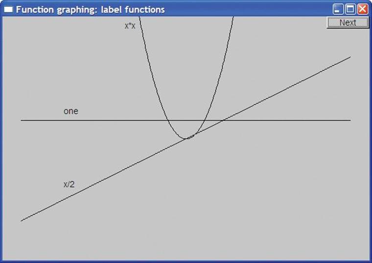
Let’s start. Let’s look at examples of what we can draw and what code it takes to draw them. In particular, look at the graphics interface classes used. Here, first, are a parabola, a horizontal line, and a sloping line:

Actually, since this chapter is about graphing functions, that horizontal line isn’t just a horizontal line; it is what we get from graphing the function
double one(double) { return 1; }
This is about the simplest function we could think of: it is a function of one argument that for every argument returns 1. Since we don’t need that argument to compute the result, we need not name it. For every x passed as an argument to one() we get the y value 1; that is, the line is defined by(x,y)==(x,1) for all x.
Like all beginning mathematical arguments, this is somewhat trivial and pedantic, so let’s look at a slightly more complicated function:
double slope(double x) { return x/2; }
This is the function that generated the sloping line. For every x, we get the y value x/2. In other words, (x,y)==(x,x/2). The point where the two lines cross is (2,1).
Now we can try something more interesting, the square function that seems to reappear regularly in this book:
double square(double x) { return x*x; }
If you remember your high school geometry (and even if you don’t), this defines a parabola with its lowest point at (0,0) and symmetric on the y axis. In other words, (x,y)==(x,x*x). So, the lowest point where the parabola touches the sloping line is (0,0).
Here is the code that drew those three functions:
constexpr int xmax = 600; // window size
constexpr int ymax = 400;
constexpr int x_orig = xmax/2; // position of (0,0) is center of window
constexpr int y_orig = ymax/2;
constexpr Point orig {x_orig,y_orig};
constexpr int r_min = -10; // range [-10:11)
constexpr int r_max = 11;
constexpr int n_points = 400; // number of points used in range
constexpr int x_scale = 30; // scaling factors
constexpr int y_scale = 30;
Simple_window win {Point{100,100},xmax,ymax,"Function graphing"};
Function s {one,r_min,r_max,orig,n_points,x_scale,y_scale};
Function s2 {slope,r_min,r_max,orig,n_points,x_scale,y_scale};
Function s3 {square,r_min,r_max,orig,n_points,x_scale,y_scale};
win.attach(s);
win.attach(s2);
win.attach(s3);
win.wait_for_button();
First, we define a bunch of constants so that we won’t have to litter our code with “magic constants.” Then, we make a window, define the functions, attach them to the window, and finally give control to the graphics system to do the actual drawing.
All of this is repetition and “boilerplate” except for the definitions of the three Functions, s, s2, and s3:
Function s {one,r_min,r_max,orig,n_points,x_scale,y_scale};
Function s2 {slope,r_min,r_max,orig,n_points,x_scale,y_scale};
Function s3 {square,r_min,r_max,orig,n_points,x_scale,y_scale};
Each Function specifies how its first argument (a function of one double argument returning a double) is to be drawn in a window. The second and third arguments give the range of x (the argument to the function to be graphed). The fourth argument (here, orig) tells the Function where the origin (0,0) is to be located within the window.
![]()
If you think that the many arguments are confusing, we agree. Our ideal is to have as few arguments as possible, because having many arguments confuses and provides opportunities for bugs. However, here we need them. We’ll explain the last three arguments later (§15.3). First, however, let’s label our graphs:
![]()
We always try to make our graphs self-explanatory. People don’t always read the surrounding text and good diagrams get moved around, so that the surrounding text is “lost.” Anything we put in as part of the picture itself is most likely to be noticed and — if reasonable — most likely to help the reader understand what we are displaying. Here, we simply put a label on each graph. The code for “labeling” was three Text objects (see §13.11):
Text ts {Point{100,y_orig-40},"one"};
Text ts2 {Point{100,y_orig+y_orig/2-20},"x/2"};
Text ts3 {Point{x_orig-100,20},"x*x"};
win.set_label("Function graphing: label functions");
win.wait_for_button();
![]()
From now on in this chapter, we’ll omit the repetitive code for attaching shapes to the window, labeling the window, and waiting for the user to hit “Next.”
However, that picture is still not acceptable. We noticed that x/2 touches x*x at (0,0) and that one crosses x/2 at (2,1) but that’s far too subtle; we need axes to give the reader an unsubtle clue about what’s going on:
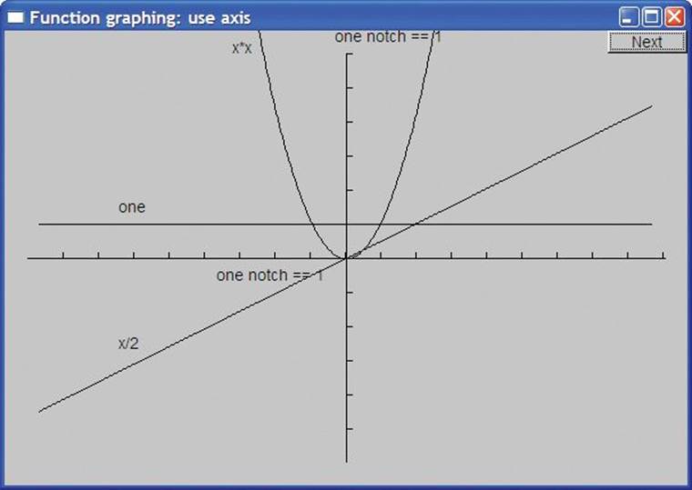
The code for the axes was two Axis objects (§15.4):
constexpr int xlength = xmax-40; // make the axis a bit smaller than the window
constexpr int ylength = ymax-40;
Axis x {Axis::x,Point{20,y_orig},
xlength, xlength/x_scale, "one notch == 1"};
Axis y {Axis::y,Point{x_orig, ylength+20},
ylength, ylength/y_scale, "one notch == 1"};
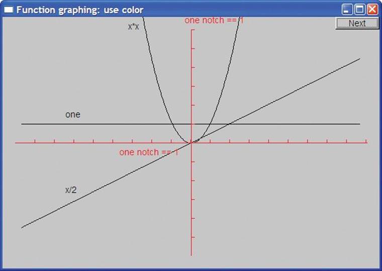
Using xlength/x_scale as the number of notches ensures that a notch represents the values 1, 2, 3, etc. Having the axes cross at (0,0) is conventional. If you prefer them along the left and bottom edges as is conventional for the display of data (see §15.6), you can of course do that instead. Another way of distinguishing the axes from the data is to use color:
x.set_color(Color::red);
y.set_color(Color::red);
And we get
![]()
This is acceptable, though for aesthetic reasons, we’d probably want a bit of empty space at the top to match what we have at the bottom and sides. It might also be a better idea to push the label for the x axis further to the left. We left these blemishes so that we could mention them — there are always more aesthetic details that we can work on. One part of a programmer’s art is to know when to stop and use the time saved on something better (such as learning new techniques or sleep). Remember: “The best is the enemy of the good.”
15.3 Function
The Function graphics interface class is defined like this:
struct Function : Shape {
// the function parameters are not stored
Function(Fct f, double r1, double r2, Point orig,
int count = 100, double xscale = 25, double yscale = 25);
};
Function is a Shape with a constructor that generates a lot of line segments and stores them in its Shape part. Those line segments approximate the values of function f. The values of f are calculated count times for values equally spaced in the [r1:r2) range:
Function::Function(Fct f, double r1, double r2, Point xy,
int count, double xscale, double yscale)
// graph f(x) for x in [r1:r2) using count line segments with (0,0) displayed at xy
// x coordinates are scaled by xscale and y coordinates scaled by yscale
{
if (r2-r1<=0) error("bad graphing range");
if (count <=0) error("non-positive graphing count");
double dist = (r2-r1)/count;
double r = r1;
for (int i = 0; i<count; ++i) {
add(Point{xy.x+int(r*xscale),xy.y-int(f(r)*yscale)});
r += dist;
}
}
The xscale and yscale values are used to scale the x coordinates and the y coordinates, respectively. We typically need to scale our values to make them fit appropriately into a drawing area of a window.
Note that a Function object doesn’t store the values given to its constructor, so we can’t later ask a function where its origin is, redraw it with different scaling, etc. All it does is to store points (in its Shape) and draw itself on the screen. If we wanted the flexibility to change a Function after construction, we would have to store the values we wanted to change (see exercise 2).
What is the type Fct that we used to represent a function argument? It is a variant of a standard library type called std::function that can “remember” a function to be called later. Fct requires its argument to be a double and its return type to be a double.
15.3.1 Default Arguments
Note the way the Function constructor arguments xscale and yscale were given initializers in the declaration. Such initializers are called default arguments and their values are used if a caller doesn’t supply values. For example:
Function s {one, r_min, r_max,orig, n_points, x_scale, y_scale};
Function s2 {slope, r_min, r_max, orig, n_points, x_scale}; // no yscale
Function s3 {square, r_min, r_max, orig, n_points}; // no xscale, no yscale
Function s4 {sqrt, r_min, r_max, orig}; // no count, no xscale, no yscale
This is equivalent to
Function s {one, r_min, r_max, orig, n_points, x_scale, y_scale};
Function s2 {slope, r_min, r_max,orig, n_points, x_scale, 25};
Function s3 {square, r_min, r_max, orig, n_points, 25, 25};
Function s4 {sqrt, r_min, r_max, orig, 100, 25, 25};
Default arguments are used as an alternative to providing several overloaded functions. Instead of defining one constructor with three default arguments, we could have defined four constructors:
struct Function : Shape { // alternative, not using default arguments
Function(Fct f, double r1, double r2, Point orig,
int count, double xscale, double yscale);
// default scale of y:
Function(Fct f, double r1, double r2, Point orig,
int count, double xscale);
// default scale of x and y:
Function(Fct f, double r1, double r2, Point orig, int count);
// default count and default scale of x or y:
Function(Fct f, double r1, double r2, Point orig);
};
![]()
It would have been more work to define four constructors, and with the four-constructor version, the nature of the default is hidden in the constructor definitions rather than being obvious from the declaration. Default arguments are frequently used for constructors but can be useful for all kinds of functions. You can only define default arguments for trailing parameters. For example:
struct Function : Shape {
Function(Fct f, double r1, double r2, Point orig,
int count = 100, double xscale, double yscale); // error
};
If a parameter has a default argument, all subsequent parameters must also have one:
struct Function : Shape {
Function(Fct f, double r1, double r2, Point orig,
int count = 100, double xscale=25, double yscale=25);
};
Sometimes, picking good default arguments is easy. Examples of that are the default for string (the empty string) and the default for vector (the empty vector). In other cases, such as Function, choosing a default is less easy; we found the ones we used after a bit of experimentation and a failed attempt. Remember, you don’t have to provide default arguments, and if you find it hard to provide one, just leave it to your user to specify that argument.
15.3.2 More examples
We added a couple more functions, a simple cosine (cos) from the standard library, and — just to show how we can compose functions — a sloping cosine that follows the x/2 slope:
double sloping_cos(double x) { return cos(x)+slope(x); }
Here is the result:
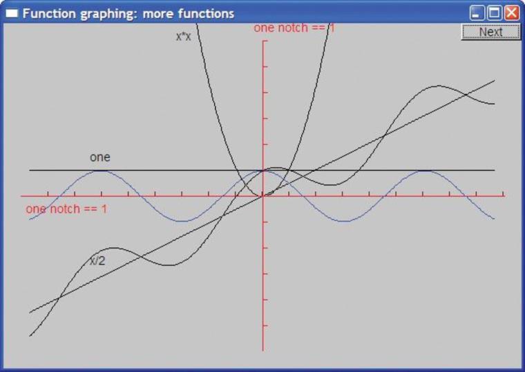
The code is
Function s4 {cos,r_min,r_max,orig,400,30,30};
s4.set_color(Color::blue);
Function s5 {sloping_cos, r_min,r_max,orig,400,30,30};
x.label.move(-160,0);
x.notches.set_color(Color::dark_red);
In addition to adding those two functions, we also moved the x axis’s label and (just to show how) slightly changed the color of its notches.
Finally, we graph a log, an exponential, a sine, and a cosine:
Function f1 {log,0.000001,r_max,orig,200,30,30}; // log() logarithm, base e
Function f2 {sin,r_min,r_max,orig,200,30,30}; // sin()
f2.set_color(Color::blue);
Function f3 {cos,r_min,r_max,orig,200,30,30}; // cos()
Function f4 {exp,r_min,r_max,orig,200,30,30}; // exp() exponential e^x
Since log(0) is undefined (mathematically, minus infinity), we started the range for log at a small positive number. The result is
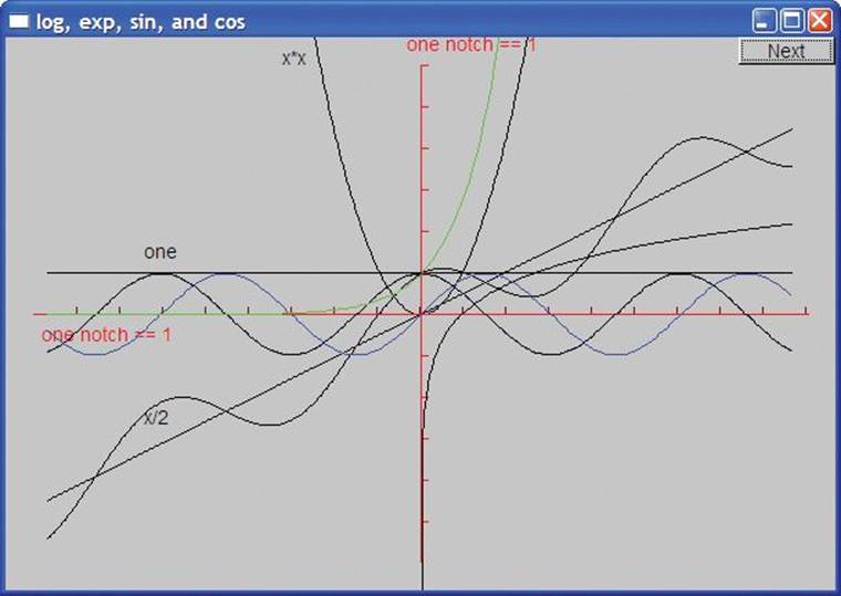
Rather than labeling those functions we used color.
Standard mathematical functions, such as cos(), sin(), and sqrt(), are declared in the standard library header <cmath>. See §24.8 and §B.9.2 for lists of the standard mathematical functions.
15.3.3 Lambda expressions
It can get tedious to define a function just to have it to pass as an argument to a Function. Consequently, C++ offers a notation for defining something that acts as a function in the argument position where it is needed. For example, we could define the sloping_cos shape like this:
Function s5 {[](double x) { return cos(x)+slope(x); },
r_min,r_max,orig,400,30,30};
The [](double x) { return cos(x)+slope(x); } is a lambda expression; that is, it is an unnamed function defined right where it is needed as an argument. The [ ] is called a lambda introducer. After the lambda introducer, the lambda expression specifies what arguments are required (the argument list) and what actions are to be performed (the function body). The return type can be deduced from the lambda body. Here, the return type is double because that’s the type of cos(x)+slope(x). Had we wanted to, we could have specified the return type explicitly:
Function s5 {[](double x) -> double { return cos(x)+slope(x); },
r_min,r_max,orig,400,30,30};
![]()
Specifying the return type for a lambda expression is rarely necessary. The main reason for that is that lambda expressions should be kept simple to avoid becoming a source of errors and confusion. If a piece of code does something significant, it should be given a name and probably requires a comment to be comprehensible to people other than the original programmer. We recommend using named functions for anything that doesn’t easily fit on a line or two.
The lambda introducer can be used to give the lambda expression access to local variables; see §15.5. See also §21.4.3.
15.4 Axis
We use Axis wherever we present data (e.g., §15.6.4) because a graph without information that allows us to understand its scale is most often suspect. An Axis consists of a line, a number of “notches” on that line, and a text label. The Axis constructor computes the axis line and (optionally) the lines used as notches on that line:
struct Axis : Shape {
enum Orientation { x, y, z };
Axis(Orientation d, Point xy, int length,
int number_of_notches=0, string label = "");
void draw_lines() const override;
void move(int dx, int dy) override;
void set_color(Color c);
Text label;
Lines notches;
};
The label and notches objects are left public so that a user can manipulate them. For example, you can give the notches a different color from the line and move() the label to a more convenient location. Axis is an example of an object composed of several semi-independent objects.
The Axis constructor places the lines and adds the “notches” if number_of_notches is greater than zero:
Axis::Axis(Orientation d, Point xy, int length, int n, string lab)
:label(Point{0,0},lab)
{
if (length<0) error("bad axis length");
switch (d){
case Axis::x:
{ Shape::add(xy); // axis line
Shape::add(Point{xy.x+length,xy.y});
if (0<n) { // add notches
int dist = length/n;
int x = xy.x+dist;
for (int i = 0; i<n; ++i) {
notches.add(Point{x,xy.y},Point{x,xy.y-5});
x += dist;
}
}
label.move(length/3,xy.y+20); // put the label under the line
break;
}
case Axis::y:
{ Shape::add(xy); // a y axis goes up
Shape::add(Point{xy.x,xy.y-length});
if (0<n) { // add notches
int dist = length/n;
int y = xy.y-dist;
for (int i = 0; i<n; ++i) {
notches.add(Point{xy.x,y},Point{xy.x+5,y});
y -= dist;
}
}
label.move(xy.x-10,xy.y-length-10); // put the label at top
break;
}
case Axis::z:
error("z axis not implemented");
}
}
Compared to much real-world code, this constructor is very simple, but please have a good look at it because it isn’t quite trivial and it illustrates a few useful techniques. Note how we store the line in the Shape part of the Axis (using Shape::add()) but the notches are stored in a separate object (notches). That way, we can manipulate the line and the notches independently; for example, we can give each its own color. Similarly, a label is placed in a fixed position relative to its axes, but since it is a separate object, we can always move it to a better spot. We use the enumerationOrientation to provide a convenient and non-error-prone notation for users.
Since an Axis has three parts, we must supply functions for when we want to manipulate an Axis as a whole. For example:
void Axis::draw_lines() const
{
Shape::draw_lines();
notches.draw(); // the notches may have a different color from the line
label.draw(); // the label may have a different color from the line
}
We use draw() rather than draw_lines() for notches and label to be able to use the color stored in them. The line is stored in the Axis::Shape itself and uses the color stored there.
We can set the color of the line, the notches, and the label individually, but stylistically it’s usually better not to, so we provide a function to set all three to the same:
void Axis::set_color(Color c)
{
Shape::set_color(c);
notches.set_color(c);
label.set_color(c);
}
Similarly, Axis::move() moves all the parts of the Axis together:
void Axis::move(int dx, int dy)
{
Shape::move(dx,dy);
notches.move(dx,dy);
label.move(dx,dy);
}
15.5 Approximation
Here we give another small example of graphing a function: we “animate” the calculation of an exponential function. The purpose is to help you get a feel for mathematical functions (if you haven’t already), to show the way graphics can be used to illustrate computations, to give you some code to read, and finally to warn about a common problem with computations.
One way of computing an exponential function is to compute the series
ex ![]() 1 + x + x2/2! + x3/3! + x4/4! + . . .
1 + x + x2/2! + x3/3! + x4/4! + . . .
The more terms of this sequence we calculate, the more precise our value of ex becomes; that is, the more terms we calculate, the more digits of the result will be mathematically correct. What we will do is to compute this sequence and graph the result after each term. The exclamation point here is used with the common mathematical meaning: factorial; that is, we graph these functions in order:
exp0(x) = 0 // no terms
exp1(x) = 1 // one term
exp2(x) = 1+x // two terms; pow(x,1)/fac(1)==x
exp3(x) = 1+x+pow(x,2)/fac(2)
exp4(x) = 1+x+pow(x,2)/fac(2)+pow(x,3)/fac(3)
exp5(x) = 1+x+pow(x,2)/fac(2)+pow(x,3)/fac(3)+pow(x,4)/fac(4)
. . .
Each function is a slightly better approximation of ex than the one before it. Here, pow(x,n) is the standard library function that returns xn. There is no factorial function in the standard library, so we must define our own:
int fac(int n) // factorial(n); n!
{
int r = 1;
while (n>1) {
r*=n;
--n;
}
return r;
}
For an alternative implementation of fac(), see exercise 1. Given fac(), we can compute the nth term of the series like this:
double term(double x, int n) { return pow(x,n)/fac(n); } // nth term of series
Given term(), calculating the exponential to the precision of n terms is now easy:
double expe(double x, int n) // sum of n terms for x
{
double sum = 0;
for (int i=0; i<n; ++i) sum+=term(x,i);
return sum;
}
Let’s use that to produce some graphics. First, we’ll provide some axes and the “real” exponential, the standard library exp(), so that we can see how close our approximation using expe() is:
Function real_exp {exp,r_min,r_max,orig,200,x_scale,y_scale};
real_exp.set_color(Color::blue);
But how can we use expe()? From a programming point of view, the difficulty is that our graphing class, Function, takes a function of one argument and expe() needs two arguments. Given C++, as we have seen it so far, there is no really elegant solution to this problem. However, lambda expressions provide a way (§15.3.3). Consider:
for (int n = 0; n<50; ++n) {
ostringstream ss;
ss << "exp approximation; n==" << n ;
win.set_label(ss.str());
// get next approximation:
Function e {[n](double x) { return expe(x,n); },
r_min,r_max,orig,200,x_scale,y_scale};
win.attach(e);
win.wait_for_button();
win.detach(e);
}
The lambda introducer, [n], says that the lambda expression may access the local variable n. That way, a call of expe(x,n) gets its n when its Function is created and its x from each call from within the Function.
Note the final detach(e) in that loop. The scope of the Function object e is the block of the for-statement. Each time we enter that block we get a new Function called e, and each time we exit the block that e goes away, to be replaced by the next. The window must not remember the old ebecause it will have been destroyed. Thus, detach(e) ensures that the window does not try to draw a destroyed object.
This first gives a window with just the axes and the “real” exponential rendered in blue:
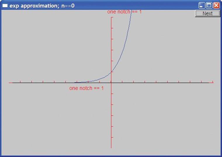
We see that exp(0) is 1 so that our blue “real exponential” crosses the y axis at (0,1).
If you look carefully, you’ll see that we actually drew the zero term approximation (exp0(x)==0) as a black line right on top of the x axis. Hitting “Next,” we get the approximation using just one term. Note that we display the number of terms used in the approximation in the window label:
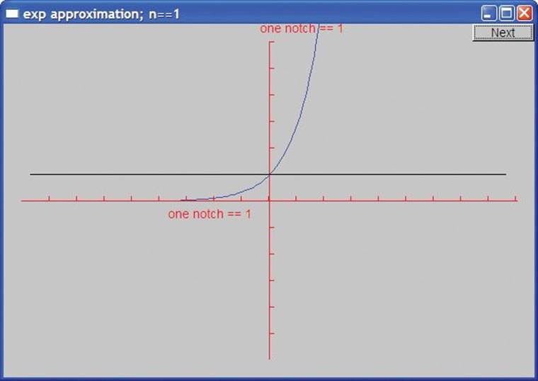
That’s the function exp1(x)==1, the approximation using just one term of the sequence. It matches the exponential perfectly at (0,1), but we can do better:
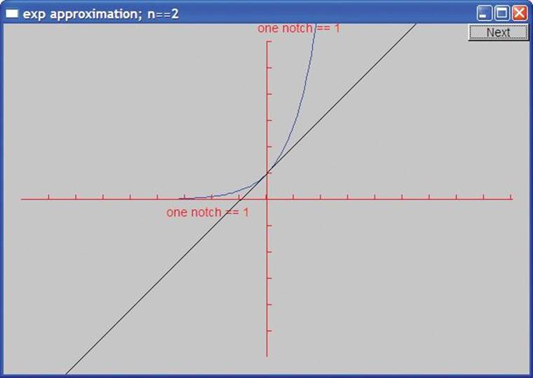
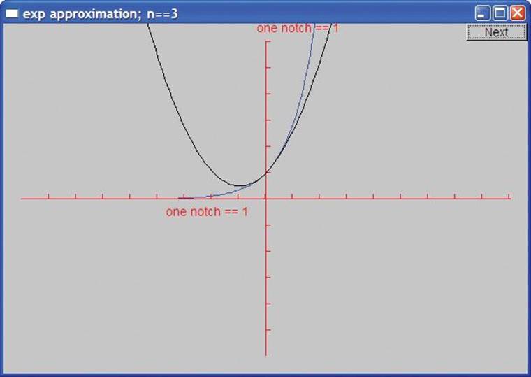
With two terms (1+x), we get the diagonal crossing the y axis at (0,1). With three terms (1+x+pow(x,2)/fac(2)), we can see the beginning of a convergence:
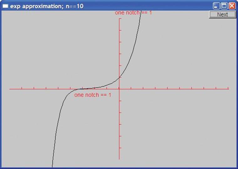
With ten terms we are doing rather well, especially for values larger than -3:
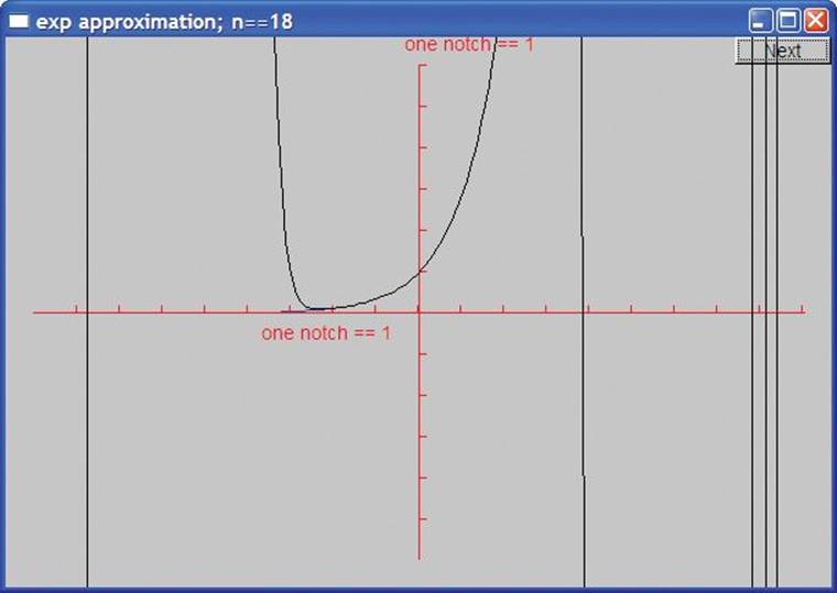
If we don’t think too much about it, we might believe that we could get better and better approximations simply by using more and more terms. However, there are limits, and after 13 terms something strange starts to happen. First, the approximations start to get slightly worse, and at 18 terms vertical lines appear:
![]()
Remember, the computer’s arithmetic is not pure math. Floating-point numbers are simply as good an approximation to real numbers as we can get with a fixed number of bits. An int overflows if you try to place a too-large integer in it, whereas a double stores an approximation. When I saw the strange output for larger numbers of terms, I first suspected that our calculation started to produce values that couldn’t be represented as doubles, so that our results started to diverge from the mathematically correct answers. Later, I realized that fac() was producing values that couldn’t be stored in an int. Modifying fac() to produce a double solved the problem. For more information, see exercise 11 of Chapter 5 and §24.2.
This last picture is also a good illustration of the principle that “it looks OK” isn’t the same as “tested.” Before giving a program to someone else to use, first test it beyond what at first seems reasonable. Unless you know better, running a program slightly longer or with slightly different data could lead to a real mess — as in this case.
15.6 Graphing data
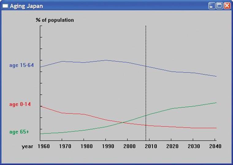
![]()
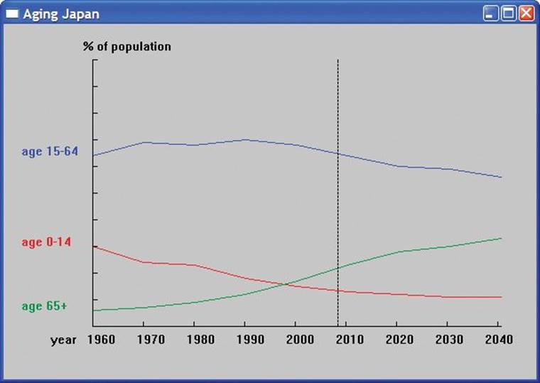
Displaying data is a highly skilled and highly valued craft. When done well, it combines technical and artistic aspects and can add significantly to our understanding of complex phenomena. However, that also makes graphing a huge area that for the most part is unrelated to programming techniques. Here, we’ll just show a simple example of displaying data read from a file. The data shown represents the age groups of Japanese people over almost a century. The data to the right of the 2008 line is a projection:
We’ll use this example to discuss the programming problems involved in presenting such data:
• Reading a file
• Scaling data to fit the window
• Displaying the data
• Labeling the graph
We will not go into artistic details. Basically, this is “graphs for geeks,” not “graphical art.” Clearly, you can do better artistically when you need to.
Given a set of data, we must consider how best to display it. To simplify, we will only deal with data that is easy to display using two dimensions, but that’s a huge part of the data most people deal with. Note that bar graphs, pie charts, and similar popular displays really are just two-dimensional data displayed in a fancy way. Three-dimensional data can often be handled by producing a series of two-dimensional images, by superimposing several two-dimensional graphs onto a single window (as is done in the “Japanese age” example), or by labeling individual points with information. If we want to go beyond that, we’ll have to write new graphics classes or adopt another graphics library.
So, our data is basically pairs of values, such as (year,number of children). If we have more data, such as (year,number of children, number of adults,number of elderly), we simply have to decide which pair of values — or pairs of values — we want to draw. In our example, we simply graphed (year,number of children), (year,number of adults), and (year,number of elderly).
![]()
There are many ways of looking at a set of (x,y) pairs. When considering how to graph such a set it is important to consider whether one value is in some way a function of the other. For example, for a (year,steel production) pair it would be quite reasonable to consider the steel production a function of the year and display the data as a continuous line. Open_polyline (§13.6) is the obvious choice for graphing such data. If y should not be seen as a function of x, for example (gross domestic product per person,population of country), Marks (§13.15) can be used to plot unconnected points.
Now, back to our Japanese age distribution example.
15.6.1 Reading a file
The file of age distributions consists of lines like this:
( 1960 : 30 64 6 )
(1970 : 24 69 7 )
(1980 : 23 68 9 )
The first number after the colon is the percentage of children (age 0-14) in the population, the second is the percentage of adults (age 15-64), and the third is the percentage of the elderly (age 65+). Our job is to read those. Note that the formatting of the data is slightly irregular. As usual, we have to deal with such details.
To simplify that task, we first define a type Distribution to hold a data item and an input operator to read such data items:
struct Distribution {
int year, young, middle, old;
};
istream& operator>>(istream& is, Distribution& d)
// assume format: ( year : young middle old )
{
char ch1 = 0;
char ch2 = 0;
char ch3 = 0;
Distribution dd;
if (is >> ch1 >> dd.year
>> ch2 >> dd.young >> dd.middle >> dd.old
>> ch3) {
if (ch1!= '(' || ch2!=':' || ch3!=')') {
is.clear(ios_base::failbit);
return is;
}
}
else
return is;
d = dd;
return is;
}
This is a straightforward application of the ideas from Chapter 10. If this code isn’t clear to you, please review that chapter. We didn’t need to define a Distribution type and a >> operator. However, it simplifies the code compared to a brute-force approach of “just read the numbers and graph them.” Our use of Distribution splits the code up into logical parts to help comprehension and debugging. Don’t be shy about introducing types “just to make the code clearer.” We define classes to make the code correspond more directly to the way we think about the concepts in our code. Doing so even for “small” concepts that are used only very locally in our code, such as a line of data representing the age distribution for a year, can be most helpful.
Given Distribution, the read loop becomes
string file_name = "japanese-age-data.txt";
ifstream ifs {file_name};
if (!ifs) error("can't open ",file_name);
// . . .
for (Distribution d; ifs>>d; ) {
if (d.year<base_year || end_year<d.year)
error("year out of range");
if (d.young+d.middle+d.old != 100)
error("percentages don't add up");
// . . .
}
That is, we try to open the file japanese-age-data.txt and exit the program if we don’t find that file. It is often a good idea not to “hardwire” a file name into the source code the way we did here, but we consider this program an example of a small “one-off” effort, so we don’t burden the code with facilities that are more appropriate for long-lived applications. On the other hand, we did put japanese-age-data.txt into a named string variable so the program is easy to modify if we want to use it — or some of its code — for something else.
The read loop checks that the year read is in the expected range and that the percentages add up to 100. That’s a basic sanity check for the data. Since >> checks the format of each individual data item, we didn’t bother with further checks in the main loop.
15.6.2 General layout
So what do we want to appear on the screen? You can see our answer at the beginning of §15.6. The data seems to ask for three Open_polylines — one for each age group. These graphs need to be labeled, and we decided to write a “caption” for each line at the left-hand side of the window. In this case, that seemed clearer than the common alternative: to place the label somewhere along the line itself. In addition, we use color to distinguish the graphs and associate their labels.
We want to label the x axis with the years. The vertical line through the year 2008 indicates where the graph goes from hard data to projected data.
We decided to just use the window’s label as the title for our graph.
![]()
Getting graphing code both correct and good-looking can be surprisingly tricky. The main reason is that we have to do a lot of fiddly calculations of sizes and offsets. To simplify that, we start by defining a set of symbolic constants that defines the way we use our screen space:
constexpr int xmax = 600; // window size
constexpr int ymax = 400;
constexpr int xoffset = 100; // distance from left-hand side of window to y axis
constexpr int yoffset = 60; // distance from bottom of window to x axis
constexpr int xspace = 40; // space beyond axis
constexpr int yspace = 40;
constexpr int xlength = xmax-xoffset-xspace; // length of axes
constexpr int ylength = ymax-yoffset-yspace;
Basically this defines a rectangular space (the window) with another rectangle (defined by the axes) within it:
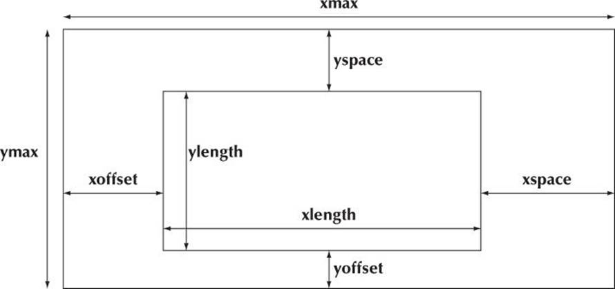
![]()
We find that without such a “schematic view” of where things are in our window and the symbolic constants that define it, we get lost and become frustrated when our output doesn’t reflect our wishes.
15.6.3 Scaling data
Next we need to define how to fit our data into that space. We do that by scaling the data so that it fits into the space defined by the axes. To do that we need the scaling factors that are the ratio between the data range and the axis range:
constexpr int base_year = 1960;
constexpr int end_year = 2040;
constexpr double xscale = double(xlength)/(end_year-base_year);
constexpr double yscale = double(ylength)/100;
We want our scaling factors (xscale and yscale) to be floating-point numbers — or our calculations could be subject to serious rounding errors. To avoid integer division, we convert our lengths to double before dividing (§4.3.3).
We can now place a data point on the x axis by subtracting its base value (1960), scaling with xscale, and adding the xoffset. A y value is dealt with similarly. We find that we can never remember to do that quite right when we try to do it repeatedly. It may be a trivial calculation, but it is fiddly and verbose. To simplify the code and minimize that chance of error (and minimize frustrating debugging), we define a little class to do the calculation for us:
class Scale { // data value to coordinate conversion
int cbase; // coordinate base
int vbase; // base of values
double scale;
public:
Scale(int b, int vb, double s) :cbase{b}, vbase{vb}, scale{s} { }
int operator()(int v) const { return cbase + (v-vbase)*scale; } // see §21.4
};
We want a class because the calculation depends on three constant values that we wouldn’t like to unnecessarily repeat. Given that, we can define
Scale xs {xoffset,base_year,xscale};
Scale ys {ymax-yoffset,0,-yscale};
Note how we make the scaling factor for ys negative to reflect the fact that y coordinates grow downward whereas we usually prefer higher values to be represented by higher points on a graph. Now we can use xs to convert a year to an x coordinate. Similarly, we can use ys to convert a percentage to a y coordinate.
15.6.4 Building the graph
Finally, we have all the prerequisites for writing the graphing code in a reasonably elegant way. We start creating a window and placing the axes:
Window win {Point{100,100},xmax,ymax,"Aging Japan"};
Axis x {Axis::x, Point{xoffset,ymax-yoffset}, xlength,
(end_year-base_year)/10,
"year 1960 1970 1980 1990 "
"2000 2010 2020 2030 2040"};
x.label.move(-100,0);
Axis y {Axis::y, Point{xoffset,ymax-yoffset}, ylength, 10,"% of population"};
Line current_year {Point{xs(2008),ys(0)},Point{xs(2008),ys(100)}};
current_year.set_style(Line_style::dash);
The axes cross at Point{xoffset,ymax-yoffset} representing (1960,0). Note how the notches are placed to reflect the data. On the y axis, we have ten notches each representing 10% of the population. On the x axis, each notch represents ten years, and the exact number of notches is calculated from base_year and end_year so that if we change that range, the axis would automatically be recalculated. This is one benefit of avoiding “magic constants” in the code. The label on the x axis violates that rule: it is simply the result of fiddling with the label string until the numbers were in the right position under the notches. To do better, we would have to look to a set of individual labels for individual “notches.”
Please note the curious formatting of the label string. We used two adjacent string literals:
"year 1960 1970 1980 1990 "
"2000 2010 2020 2030 2040"
Adjacent string literals are concatenated by the compiler, so that’s equivalent to
"year 1960 1970 1980 1990 2000 2010 2020 2030 2040"
That can be a useful “trick” for laying out long string literals to make our code more readable.
The current_year is a vertical line that separates hard data from projected data. Note how xs and ys are used to place and scale the line just right.
Given the axes, we can proceed to the data. We define three Open_polylines and fill them in the read loop:
Open_polyline children;
Open_polyline adults;
Open_polyline aged;
for (Distribution d; ifs>>d; ) {
if (d.year<base_year || end_year<d.year) error("year out of range");
if (d.young+d.middle+d.old != 100)
error("percentages don't add up");
const int x = xs{d.year};
children.add(Point{x,ys(d.young)});
adults.add(Point{x,ys(d.middle)});
aged.add(Point{x,ys(d.old)});
}
The use of xs and ys makes scaling and placement of the data trivial. “Little classes,” such as Scale, can be immensely important for simplifying notation and avoiding unnecessary repetition — thereby increasing readability and increasing the likelihood of correctness.
To make the graphs more readable, we label each and apply color:
Text children_label {Point{20,children.point(0).y},"age 0-14"};
children.set_color(Color::red);
children_label.set_color(Color::red);
Text adults_label {Point{20,adults.point(0).y},"age 15-64"};
adults.set_color(Color::blue);
adults_label.set_color(Color::blue);
Text aged_label {Point{20,aged.point(0).y},"age 65+"};
aged.set_color(Color::dark_green);
aged_label.set_color(Color::dark_green);
Finally, we need to attach the various Shapes to the Window and start the GUI system (§14.2.3):
win.attach(children);
win.attach(adults);
win.attach(aged);
win.attach(children_label);
win.attach(adults_label);
win.attach(aged_label);
win.attach(x);
win.attach(y);
win.attach(current_year);
gui_main();
All the code could be placed inside main(), but we prefer to keep the helper classes Scale and Distribution outside together with Distribution’s input operator.
In case you have forgotten what we were producing, here is the output again:
 Drill
Drill
Function graphing drill:
1. Make an empty 600-by-600 Window labeled “Function graphs.”
2. Note that you’ll need to make a project with the properties specified in the “installation of FLTK” note from the course website.
3. You’ll need to move Graph.cpp and Window.cpp into your project.
4. Add an x axis and a y axis each of length 400, labeled “1 = = 20 pixels” and with a notch every 20 pixels. The axes should cross at (300,300).
5. Make both axes red.
In the following, use a separate Shape for each function to be graphed:
1. Graph the function double one(double x) { return 1; } in the range [-10,11] with (0,0) at (300,300) using 400 points and no scaling (in the window).
2. Change it to use x scale 20 and y scale 20.
3. From now on use that range, scale, etc. for all graphs.
4. Add double slope(double x) { return x/2; } to the window.
5. Label the slope with a Text "x/2" at a point just above its bottom left end point.
6. Add double square(double x) { return x*x; } to the window.
7. Add a cosine to the window (don’t write a new function).
8. Make the cosine blue.
9. Write a function sloping_cos() that adds a cosine to slope() (as defined above) and add it to the window.
Class definition drill:
1. Define a struct Person containing a string name and an int age.
2. Define a variable of type Person, initialize it with “Goofy” and 63, and write it to the screen (cout).
3. Define an input (>>) and an output (<<) operator for Person; read in a Person from the keyboard (cin) and write it out to the screen (cout).
4. Give Person a constructor initializing name and age.
5. Make the representation of Person private, and provide const member functions name() and age() to read the name and age.
6. Modify >> and << to work with the redefined Person.
7. Modify the constructor to check that age is [0:150) and that name doesn’t contain any of the characters ; : " ' [ ] * & ^ % $ # @ !. Use error() in case of error. Test.
8. Read a sequence of Persons from input (cin) into a vector<Person>; write them out again to the screen (cout). Test with correct and erroneous input.
9. Change the representation of Person to have first_name and second_name instead of name. Make it an error not to supply both a first and a second name. Be sure to fix >> and << also. Test.
Review
1. What is a function of one argument?
2. When would you use a (continuous) line to represent data? When do you use (discrete) points?
3. What function (mathematical formula) defines a slope?
4. What is a parabola?
5. How do you make an x axis? A y axis?
6. What is a default argument and when would you use one?
7. How do you add functions together?
8. How do you color and label a graphed function?
9. What do we mean when we say that a series approximates a function?
10. Why would you sketch out the layout of a graph before writing the code to draw it?
11. How would you scale your graph so that the input will fit?
12. How would you scale the input without trial and error?
13. Why would you format your input rather than just having the file contain “the numbers”?
14. How do you plan the general layout of a graph? How do you reflect that layout in your code?
Terms
approximation
default argument
function
lambda
scaling
screen layout
Exercises
1. Here is another way of defining a factorial function:
int fac(int n) { return n>1 ? n*fac(n-1) : 1; } // factorial n!
It will do fac(4) by first deciding that since 4>1 it must be 4*fac(3), and that’s obviously 4*3*fac(2), which again is 4*3*2*fac(1), which is 4*3*2*1. Try to see that it works. A function that calls itself is said to be recursive. The alternative implementation in §15.5 is called iterativebecause it iterates through the values (using while). Verify that the recursive fac() works and gives the same results as the iterative fac() by calculating the factorial of 0, 1, 2, 3, 4, up until and including 20. Which implementation of fac() do you prefer, and why?
2. Define a class Fct that is just like Function except that it stores its constructor arguments. Provide Fct with “reset” operations, so that you can use it repeatedly for different ranges, different functions, etc.
3. Modify Fct from the previous exercise to take an extra argument to control precision or whatever. Make the type of that argument a template parameter for extra flexibility.
4. Graph a sine (sin()), a cosine (cos()), the sum of those (sin(x)+cos(x)), and the sum of the squares of those (sin(x)*sin(x)+cos(x)*cos(x)) on a single graph. Do provide axes and labels.
5. “Animate” (as in §15.5) the series 1-1/3+1/5-1/7+1/9-1/11+ . . . . It is known as Leibniz’s series and converges to pi/4.
6. Design and implement a bar graph class. Its basic data is a vector<double> holding N values, and each value should be represented by a “bar” that is a rectangle where the height represents the value.
7. Elaborate the bar graph class to allow labeling of the graph itself and its individual bars. Allow the use of color.
8. Here is a collection of heights in centimeters together with the number of people in a group of that height (rounded to the nearest 5cm): (170,7), (175,9), (180,23), (185,17), (190,6), (195,1). How would you graph that data? If you can’t think of anything better, do a bar graph. Remember to provide axes and labels. Place the data in a file and read it from that file.
9. Find another data set of heights (an inch is 2.54cm) and graph them with your program from the previous exercise. For example, search the web for “height distribution” or “height of people in the United States” and ignore a lot of rubbish or ask your friends for their heights. Ideally, you don’t have to change anything for the new data set. Calculating the scaling from the data is a key idea. Reading in labels from input also helps minimize changes when you want to reuse code.
10. What kind of data is unsuitable for a line graph or a bar graph? Find an example and find a way of displaying it (e.g., as a collection of labeled points).
11. Find the average maximum temperatures for each month of the year for two or more locations (e.g., Cambridge, England, and Cambridge, Massachusetts; there are lots of towns called “Cambridge”) and graph them together. As ever, be careful with axes, labels, use of color, etc.
Postscript
Graphical representation of data is important. We simply understand a well-crafted graph better than the set of numbers that was used to make it. Most people, when they need to draw a graph, use someone else’s code — a library. How are such libraries constructed and what do you do if you don’t have one handy? What are the fundamental ideas underlying “an ordinary graphing tool”? Now you know: it isn’t magic or brain surgery. We covered only two-dimensional graphs; three-dimensional graphing is also very useful in science, engineering, marketing, etc. and can be even more fun. Explore it someday!
All materials on the site are licensed Creative Commons Attribution-Sharealike 3.0 Unported CC BY-SA 3.0 & GNU Free Documentation License (GFDL)
If you are the copyright holder of any material contained on our site and intend to remove it, please contact our site administrator for approval.
© 2016-2026 All site design rights belong to S.Y.A.