Joe Celko's Complete Guide to NoSQL: What Every SQL Professional Needs to Know about NonRelational Databases (2014)

Chapter 5. Streaming Databases and Complex Events

Abstract

Streaming databases use traditional structured data, but add a temporal dimension to it. If RDBMS is static data and static processing, then streaming data is moving data and active processing. It has to use a generational concurrency model to catch the flow of data. These databases do not want to respond to a query; the database is taking action. The database monitors a system or process by looking for exceptional behavior and generates alerts when such behavior occurs. When an event is observed, the system has to deliver the right information to the right consumer at the right granularity at the right time. It is personalized information delivery. From this, the consumer can decide on some dynamic operational behavior.

Keywords

dynamic operational behavior; CEP (complex event processing); generational concurrency model; information dissemination; isolation levels in optimistic concurrency; observation; speed; velocity; streaming database; Q language

Introduction

This chapter discusses streaming databases. These tools are concerned with data that is moving through time and has to be “caught” as it flows in the system. Rather than static data, we look for patterns of events in this temporal flow. Again, this is not a computational model for data.

The relational model assumes that the tables are static during a query and that the result is also a static table. If you want a mental picture, think of a reservoir of data that is used as it stands at the time of the query or other Data Manipulation Language (DML) statement. This is, roughly, the traditional RDBMS.

But streaming databases are built on constantly flowing data; think of a river or a pipe of data. The best-known examples of streaming data are stock and commodity trading done by software in subsecond trades. The reason that these applications are well known is because when they mess up, it appears in the newspapers. To continue the water/data analogy, everyone knows when a pipe breaks or a toilet backs up.

A traditional RDBMS, like a static reservoir, is concerned with data volume. Vendors talk about the number of terabytes (or petabytes or exabytes these days) their product can handle. Transaction volume and response time are secondary. They advertise and benchmark under the assumption that a traditional OLTP system can be made “good enough” with existing technology.

A streaming database, like a fire hose, is concerned with data volume, but more important are flow rate, speed, and velocity. There is a fundamental difference between a bathtub that fills at the rate of 10 liters per minute versus a drain pipe that flows at the rate of 100 liters per minute. There is also a difference between the wide pipe and the narrow nozzle of an industrial pressure cutter at the rate of 100 liters per second.

5.1 Generational Concurrency Models

Databases have to support concurrent users. Sharing data is a major reason to use DBMS; a single user is better off with a file system. But this means we need some kind of “traffic control” in the system.

This concept came from operating systems that had to manage hardware. Two jobs should not be writing to the same printer at the same time because it would produce a garbage printout. Reading data from an RDBMS is not a big problem, but when two sessions want to update, delete, or insert data in the same table, it is not so easy.

5.1.1 Optimistic Concurrency

Optimistic concurrency control assumes that conflicts are exceptional and we have to handle them after the fact. The model for optimistic concurrency is microfilm! Most database people today have not even seen microfilm, so, if you have not, you might want to Google it. This approach predates databases by decades. It was implemented manually in the central records department of companies when they started storing data on microfilm. A user did not get the microfilm, but instead the records manager made a timestamped photocopy for him. The user took the copy to his desk, marked it up, and returned it to the central records department. The central records clerk timestamped the updated document, photographed it, and added it to the end of the roll of microfilm.

But what if a second user, user B, also went to the central records department and got a timestamped photocopy of the same document? The central records clerk had to look at both timestamps and make a decision. If user A attempted to put his updates into the database while user B was still working on her copy, then the clerk had to either hold the first copy, wait for the second copy to show up, or return the second copy to user A. When both copies were in hand, the clerk stacked the copies on top of each other, held them up to the light, and looked to see if there were any conflicts. If both updates could be made to the database, the clerk did so. If there were conflicts, the clerk must either have rules for resolving the problems or reject both transactions. This represents a kind of row-level locking, done after the fact.

The copy has a timestamp on it; call it t₀ or start_timestamp. The changes are committed by adding the new version of the data to the end of the file with a timestamp, t₁. That is unique within the system. Since modern machinery can work with nanoseconds, an actual timestamp and not just a sequential numbering will work. If you want to play with this model, you can get a copy of Borland’s Interbase or its open source, Firebird.

5.1.2 Isolation Levels in Optimistic Concurrency

A transaction running on its private copy of the data is never blocked. But this means that at any time, each data item might have multiple versions, created by active and committed transactions.

When transaction T1 is ready to commit, it gets a commit_timestamp that is later than any existing start_timestamp or commit_timestamp. The transaction successfully COMMITs only if no other transaction, say T2, with a commit_timestamp in T1’s temporal interval [start_timestamp, commit_timestamp] wrote data that T1 also wrote. Otherwise, T1 will ROLLBACK. This first-committer-wins strategy prevents lost updates (phenomenon P4). When T1 COMMITs, its changes become visible to all transactions of which the start_timestamps are larger than T1’s commit_timestamp. This is called snapshot isolation, and it has its own problems.

Snapshot isolation is nonserializable because a transaction’s reads come at one instant and the writes at another. Assume you have several transactions working on the same data and a constraint that (x + y > 0) on the table. Each transaction that writes a new value for x and y is expected to maintain the constraint. While T1 and T2 both act properly in isolation with their copy, the constraint fails to hold when you put them together. The possible problems are:

◆ A5 (data item constraint violation): Suppose constraint C is a database constraint between two data items x and y in the database. There are two anomalies arising from constraint violation.

◆ A5A (read skew): Suppose transaction T1 reads x, and then T2 updates x and y to new values and COMMITs. Now, if T1 reads y, it may see an inconsistent state, and therefore produce an inconsistent state as output.

◆ A5B (write skew): Suppose T1 reads x and y, which are consistent with constraint C, and then T2 reads x and y, writes x, and COMMITs. Then T1 writes y. If there were a constraint between x and y, it might be violated.

◆ P2 (fuzzy reads): This is a degenerate form of A5A, where (x = y). More typically, a transaction reads two different but related items (e.g., referential integrity).

◆ A5B (write skew): This could arise from a constraint at a bank, where account balances are allowed to go negative as long as the sum of commonly held balances remains non-negative.

Clearly, neither A5A nor A5B could arise in histories where P2 is precluded, since both A5A and A5B have T2 write a data item that has been previously read by an uncommitted T1. Thus, phenomena A5A and A5B are only useful for distinguishing isolation levels below REPEATABLE READ in strength.

The ANSI SQL definition of REPEATABLE READ, in its strict interpretation, captures a degenerate form of row constraints, but misses the general concept. To be specific, Locking a table with a transaction level of REPEATABLE READ provides protection from Row Constraint Violations but the ANSI SQL definition forbidding anomalies A1 and A2, does not. Snapshot Isolation is even stronger than READ COMMITTED.

The important property for here is that you can be reading data at timestamp t_n while changing data at timestamp t_{(n + k)} in parallel. You are drinking from a different part of the stream and can reconstruct a consistent view of the database at any point in the past.

Table 5.1

ANSI SQL Isolation Levels Defined in Terms of the Three Original Phenomena

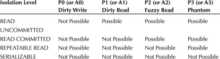
Table 5.2

Degrees of Consistency and Locking Isolation Levels Defined in Terms of Locks

5.2 Complex Event Processing

The other assumption of a traditional RDBMS is that the constraints on the data model are always in effect when you query. All the water is in one place and ready to drink. But the stream data model deals with complex event processing (CEP). That means that not all the data has arrived in the database yet! You cannot yet complete a query because you are anticipating data, but you know you have part of it. The data can be from the same source, or from multiple sources.

The event concept is delightfully explained in an article by Gregor Hohpe (2005). Imagine you are in a coffee shop. Some coffee shops are synchronous: a customer walks up to the counter and asks for coffee and pastry; the person behind the counter puts the pastry into the microwave, prepares the coffee, takes the pastry out of the microwave, takes the payment, gives the tray to the customer, and then turns to serve the next customer. Each customer is a single thread.

Some coffee shops are asynchronous: the person behind the counter takes the order and payment and then moves on to serve the next customer; a short-order cook heats the pastry and a barista makes the coffee. When both coffee and pastry are ready, they call the customer for window pickup or send a server to the table with the order. The customer can sit down, take out a laptop, and write books while waiting.

The model has producers and consumers, or input and output streams. The hot pastry is an output that goes to a consumer who eats it. The events can be modeled in a data flow diagram if you wish.

In both shops, this is routine expected behavior. Now imagine a robber enters the coffee shop and demands people’s money. This is not, I hope, routine expected behavior. The victims have to file a police report and will probably call credit card companies to cancel stolen credit cards. These events will trigger further events, such as a court appearance, activation of a new credit card, and so forth.

5.2.1 Terminology for Event Processing

It is always nice to have terminology when we talk, so let’s discuss some. A situation is an event that might require a response. In the coffee shop example, running low on paper cups is an event that might not require an immediate response yet. (“How is the cup situation? We’re low!”) However, running out of paper cups is an event that does require a response since you cannot sell coffee without them. The pattern is detect → decide → respond, either by people or by machine.

1. Observation: Event processing is used to monitor a system or process by looking for exceptional behavior and generating alerts when such behavior occurs. In such cases, the reaction, if any, is left to the consumers of the alerts; the job of the event processing application is to produce the alerts only.

2. Information dissemination: When an event is observed, the system has to deliver the right information to the right consumer at the right granularity at the right time. It is personalized information delivery. My favorite is the emails I get from my banks about my checking accounts. One bank lets me set a daily limit and would only warn me if I went over the limit. Another bank sends me a short statement of yesterday’s transactions each day. They do not tell my wife about my spending or depositing, just me.

3. Dynamic operational In this model, the actions of the system are automatically driven by the incoming events. The online trading systems use this model. Unfortunately, a system does not have to have good judgment and needs a way to prevent endless feedback. This situation lead to Amazon’s $23,698,655.93 book about flies in 2011. Here is the story: It regards Peter Lawrence’s The Making of a Fly, a biology book about flies, which published in 1992 and is out of print. But Amazon listed 17 copies for sale: 15 used from $35.54, and 2 new from two legitimate booksellers. The prices kept rising over several days, slowly converging in a pattern. The copy offered by Bordeebook was 1.270589 times the price of the copy offered by Profnath. Once a day Profnath set their price to be 0.9983 times higher than Bordeebook’s price. The prices would remain close for several hours, until Bordeebook “noticed” Profnath’s change and elevated their price to 1.270589 times Profnath’s higher price.

Amazon retailers are increasingly using algorithmic pricing (something Amazon itself does on a large scale), with a number of companies offering pricing algorithms/services to retailers that do have a sanity check. The Profnath algorithm wants to make their price one of the lowest price, but only by a tiny bit so it will sort to the top of the list. A lot of business comes from being in first three positions!

On the other hand, Bordeebook has lots of positive feedback, so their algorithm bets that buyers will pay a premium for that level of confidence. Back in the days when I owned bookstores, there were “book scouts” who earned their living by searching through catalogs and bookstores and buying books for clients. Bordeebook’s algorithm seems to be a robot version of the book scout, with a markup of 1.270589 times the price of the book.

4. Active diagnostics: The event processing application diagnoses a problem by observing symptoms. A help desk call is the most common example for most of us. There is a classic Internet joke about the world’s first help desk (http://www.why-not.com/jokes.old/archive/1998/january/27.html) that begins with “This fire help. Me Groog”; “Me Lorto. Help. Fire not work,” with the punchline being Grogg beating Lorto with a club for being too stupid to live.

Manufacturing systems look for product failures based on observable symptoms. The immediate goal is to correct flaws in the process but the real goal is to find the root cause of these symptoms. If you view manufacturing as a stream, you will learn about a statistical sampling teaching called sequential analysis, invented by Abraham Wald (1973) for munitions testing. (The basic idea is that testing bullets, light bulbs, and many other goods is destructive, so we want to pull the smallest sample size from the stream that will give us the confidence level we want. But the sample size does not have to be constant! If we have a lot of failures, then we want to increase the sample size; if the failure rate is low, we can reduce the test sample size. A technique called Haldanes’ inverse samplingplays into the adjustment, if you want to do more research.

This idea actually goes back to the early days of statistics under the modern name “gambler’s ruin” in the literature. A gambler who raises his bet to a fixed fraction of bankroll when he wins, but does not reduce his bet when he loses, will eventually go broke, even if he has a positive expected value on each bet. There are problems that can only be solved with sequential analysis.

5. Predictive processing: You want to identify events before they have happened, so you can eliminate their consequences; in fact, the events might not actually exist! Imagine a fraud detection system in a financial institution that looks for patterns. It will act when it suspects fraud and possibly generate false positives, so further investigation will be required before you can be sure whether a fraud has actually taken place or not. The classic examples in finance are employees who do not take vacations (embezzlers), customers who suddenly apply for lots of credit cards (about to go bankrupt), and changes in purchase patterns (stolen identity).

These different classes of events do not exclude each other, so an application may fall into several of these categories.

5.2.2 Event Processing versus State Change Constraints

The event model is not quite the same as a state transition model for a system. State transitions are integrity checks that assure data changes only according to rules for sequences of procedures, of fixed or variable lifespans, warranties, commercial offers, and bids. You can use the Data Declaration Language (DDL) constraints in SQL to assure the state transition constraints via an auxiliary table. I do not go into much detail here since this is more of an SQL programming topic.

Such constraints can be modeled as a state-transition diagram to enforce the rules when an entity can be updated only in certain ways. There is an initial state, flow lines that show what are the next legal states, and one or more termination states. The original example was a simple state change diagram of possible marital states that looked like Figure 5.1.

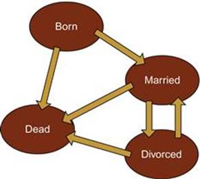
FIGURE 5.1 Martial Status State Transitions.

Here is a skeleton DDL with the needed FOREIGN KEY reference to valid state changes and the date that the current state started for me:

CREATE TABLE MyLife

(previous_state VARCHAR(10) NOT NULL,

current_state VARCHAR(10) NOT NULL,

CONSTRAINT Valid_State_Change

FOREIGN KEY (previous_state, current_state)

REFERENCES StateChanges (previous_state, current_state),

start_date DATE NOT NULL PRIMARY KEY,

––etc.);

These are states of being locked into a rigid pattern. The initial state in this case is “born” and the terminal state is “dead,” a very terminal state of being. There is an implied temporal ordering, but no timestamps to pinpoint them in time. An acorn becomes an oak tree before it becomes lumber and finally a chest of drawers. The acorn does not jump immediately to being a chest of drawers. This is a constraint and not an event; there is no action per se.

5.2.3 Event Processing versus Petri Nets

A Petri net is a mathematical model of a system that is handy for CEP. There is a lot of research on them and they are used to design computer systems with complex timing problems. A Petri net consists of places (shown as circles), transitions (shown as lines or bars), and arcs (directed arrows).

Arcs run from a place to a transition or vice versa, never between places or between transitions. The places from which an arc runs to a transition are called the input places of the transition; the places to which arcs run from a transition are called the output places of the transition.

Graphically, places in a Petri net contain zero or more tokens (shown as black dots). The tokens will move around the Petri when a transition fires. A transition of a Petri net may fire whenever there are sufficient tokens at the start of all input arcs. When a transition fires, it consumes these input tokens, and places new tokens in the places at the end of all output arcs in an atomic step.

Petri nets are nondeterministic: when multiple transitions are enabled at the same time, any one of them may fire. If a transition is enabled, it may fire, but it doesn’t have to. Multiple tokens may be present anywhere in the net (even in the same place).

Petri nets can model the concurrent behavior of distributed systems where there is no central control. Fancier versions of this technique have inhibitor arcs, use colored tokens, and so forth. But the important point is that you can prove that a Petri net can be designed to come to a stable state from any initial marking. The classic textbook examples are a two-way traffic light and the dining philosophers problem. You can see animations of these Petri nets at http://www.informatik.uni-hamburg.de/TGI/PetriNets/introductions/aalst/.

The dining philosophers problem was due to Edsger Dijkstra as a 1965 student exam question, but Tony Hoare gave us the present version of it. Five philosophers sit at a table with a bowl of rice in front of each of them. A chopstick is placed between each pair of adjacent philosophers. Each philosopher must alternately think and eat. However, a philosopher can only eat rice when he or she has a pair of chopsticks. Each chopstick can be held by only one philosopher and so a philosopher can use a chopstick only if it’s not being used by another philosopher. After he or she finishes eating, a philosopher needs to put down both chopsticks so they become available to others. A philosopher can grab the chopstick on his or her right or left as they become available, but cannot start eating before getting both of them. Assume the rice bowls are always filled.

No philosopher has any way of knowing what the others will do. The problem is how to keep the philosophers forever alternating between eating and thinking and not have anyone starve to death.

5.3 Commercial Products

You can find commercial products from IBM (SPADE), Oracle (Oracle CEP), Microsoft (StreamInsight), and smaller vendors, such as StreamBase (stream-oriented extension of SQL) and Kx (Q language, based on APL), as well as open-source projects (Esper, stream-oriented extension of SQL).

Broadly speaking, the languages are SQL-like and readable, or they are C-like and cryptic. As examples of the two extremes, let’s look at StreamBase and Kx.

5.3.1 StreamBase¹

StreamBase makes direct extensions to a basic version of SQL that will be instantly readable to an SQL programmer. As expected, the keyword CREATE adds persistent objects to the schema; here is partial list of DDL statements:

CREATE SCHEMA

CREATE TABLE

CREATE INPUT STREAM

CREATE OUTPUT STREAM

CREATE STREAM

CREATE ERROR INPUT STREAM

CREATE ERROR OUTPUT STREAM

Notice that streams are declared for input and output and for error handling. Each table can be put in MEMORY or DISK. Each table must have a PRIMARY KEY that that be implemented with a [USING {HASH | BTREE}] clause. Secondary indexes are optional and are declared with a CREATE INDEX statement.

The data types are more like Java than SQL. There are the expected types of BOOL, BLOB, DOUBLE, INT, LONG, STRING, and TIMESTAMP. But they include structured data types (LIST, TUPLE, BLOB) and special types that apply to the StreamBase engine (CAPTURE, named schema data type, etc.). The TIMESTAMP is the ANSI style date and time data type, and also can be used as an ANSI interval data type. The STRING is not a fixed-length data type, as in SQL. BOOL can be {TRUE, FALSE}.

The extensions for streams are logical. For example, we can use a statement to declare dynamic variables that get their values from a stream. Think of a ladle dipping into a stream with the following syntax:

DECLARE < variable_identifier > < data type > DEFAULT < default_value >

[UPDATE FROM '('stream_query')'];

In this example, the dynamic variable dynamic_var changes value each time a tuple is submitted to the input stream Dyn_In_Stream. In the SELECT clause that populates the output stream, the dynamic variable is used as an entry in the target list as well as in the WHEREclause predicate:

CREATE INPUT STREAM Dyn_In_Stream (current_value INT);

DECLARE dynamic_var INT DEFAULT 15 UPDATE FROM

(SELECT current_value FROM Dyn_In_Stream);

CREATE INPUT STREAM Students

(student_name STRING, student_address STRING, student_age INT);

CREATE OUTPUT STREAM Selected_Students AS

SELECT *, dynamic_var AS minimum_age FROM Students WHERE age > = dynamic_val;

One interesting streaming feature is the metronome and heartbeat. It is such a good metaphor. Here is the syntax:

CREATE METRONOME < metronome_identifier > (< field_identifier >, < interval >);

The < field_identifier > is a tuple field that will contain the timestamp value. The < interval > is an integer value in seconds. The METRONOME delivers output tuples periodically based on the system clock. In the same way that a musician’s metronome can be used to indicate the exact tempo of a piece of music, METRONOME can be used to control the timing of downstream operations.

At fixed intervals, a METRONOME will produce a tuple with a single timestamp field named < field_identifier > that will contain the current time value from the system clock on the computer hosting the StreamBase application. A METRONOME begins producing tuples as soon as the application starts.

Its partner is the HEARTBEAT statement, with this syntax:

< stream expression >

WITH HEARTBEAT ON < field_identifier >

EVERY < interval > [SLACK < timeout >]

INTO < stream_identifier >

[ERROR INTO < stream_identifier >]

The < field_identifier > is the field in the input stream that holds a timestamp data type. The < interval > is the value in decimal seconds at which the heartbeat emits tuples. The < timeout > is the value in decimal seconds that specifies a permissible delay in receiving the data tuple.

HEARTBEAT adds timer tuples on the same stream with your data tuples so that downstream operations can occur even if there is a lull in the incoming data. HEARTBEAT detects late or missing tuples. Like METRONOME, HEARTBEAT uses the system clock and emits output tuples periodically, but HEARTBEAT can also emit tuples using information in the input stream, independent of the system clock.

HEARTBEAT passes input tuples directly through to the output stream, updating its internal clock. If an expected input tuple does not arrive within the configured < interval > plus a < timeout > value, then HEARTBEAT synthesizes a tuple, with all NULL data fields except for the timestamp, and emits it.

HEARTBEAT sits on a stream and passes through data tuples without modification. The data tuple must include a field of type < timestamp >. At configurable intervals, HEARTBEAT inserts a tuple with the same schema as the data tuple onto the stream. Fields within tuples that originate from the HEARTBEAT are set to NULL, with the exception of the < timestamp > field, which always has a valid value.

HEARTBEAT does not begin to emit tuples until the first data tuple has passed along the stream. HEARTBEAT emits a tuple whenever the output < interval > elapses on the system clock or whenever the data tuple’s < timestamp > field crosses a multiple of the output < interval >. If a data tuple’s < timestamp > field has a value greater than the upcoming HEARTBEAT < interval >, HEARTBEAT immediately emits as many tuples as needed to bring its < timestamp > in line with the < timestamp > values currently on the stream.

HEARTBEAT generates a stream and can be used anywhere a stream expression is acceptable. The following example illustrates the use of HEARTBEAT:

CREATE INPUT STREAM Input_Trades

(stock_symbol STRING,

stock_price DOUBLE,

trade_date TIMESTAMP);

CREATE OUTPUT STREAM Output_Trades_Trades;

CREATE ERROR Output_Trades STREAM Flameout;

This can be used with a query, like this:

SELECT * FROM Input_Trades

WITH HEARTBEAT ON trade_date

EVERY 10.0 SLACK 0.5

INTO Output_Trades

ERROR INTO Flameout;

There are many more features to work with the streams. The stream can be partitioned into finite blocks of tuples with the CREATE [MEMORY | DISK] MATERIALIZED WINDOW < window name >, and these subsets of an infinite stream can be used much like a table. Think of a bucket drawing data from a stream. The BSORT can reorder slightly disordered streams by applying a user-defined number of sort passes over a buffer. BSORT produces a new, reordered stream. There are other tools, but this is enough for an overview.

While you can write StreamSQL as a text file and compile it, the company provides a graphic tool, StreamBase Studio, that lets you draw a “plumbing diagram” to produce the code. The diagram is also good documentation for a project.

5.3.2 Kx²

Q is a proprietary array processing language developed by Arthur Whitney and commercialized by Kx Systems. The Kx products have been in use in the financial industry for over two decades. The language serves as the query language for kdb +, their disk-based/in-memory, columnar database.

The Q language evolved from K, which evolved from APL, short for A Programming Language, developed by Kenneth E. Iverson and associates. It enjoyed a fad with IBM and has special keyboards for the cryptic notation that features mix of Greek, math, and other special symbols.

One of the major problems with APL was the symbols. IBM Selectric typeball could only hold 88 characters and APL has more symbols than that, so you had to use overstrikes. Q, on the other hand, uses the standard ASCII character set.

This family of languages uses a model of atoms, lists, and functions taken in part from LISP. Atoms are indivisible scalars and include numeric, character, and temporal data types. Lists are ordered collections of atoms (or other lists) upon which the higher-level data structures like dictionaries and tables are internally constructed. The operators in the language are functions that use whole structures as inputs and outputs. This means that there is no operator precedence; the code is excluded from right to left, just like nested function calls in mathematics. Think about how you evaluate sin(cos(x)) in math; first compute the cosine of x, then apply the sine to that result. The parentheses will become a mess, so we also use the notation fg (x) for functional composition in math. In Q, they are simply written in sequence.

The data types are the expected ones (given with the SQL equivalents shortly), but the temporal types are more complete than you might see in other languages. The numerics are Boolean (BIT), byte (SMALLINT), int (INTEGER), long (BIGINT), real (FLOAT), and float (DOUBLE PRECISION). The string tapes are char (CHAR(1)) and symbol (VARCHAR(n)). The temporal data types are date (DATE), date time (TIMESTAMP), minute (INTERVAL), second (INTERVAL), and time (TIME).

The language also uses the IEEE floating-point standard infinities and NaN values. If you do not know about them, then you need to do some reading. These are special values that represent positive and negative infinities, and thing that are “not a number” with special rules for their use.

There is also an SQL style “select [p] [by p] from texp [where p]” expression. The by clause is a change in the usual SQL syntax, best shown with an example. Start with a simple table:

tdetails

eid | name iq

----| --------------

1001| Dent 98

1002| Beeblebrox 42

1003| Prefect 126

The following statement and its results are shown below. The count.. by.. sorts the rows by iq and returns the relative position in the table. The max is the highest value of sc in the from clause table:

select topsc:max sc, cnt:count sc by eid.name from tdetails where eid.name <> `Prefect

name | topsc cnt

----------| ---------

Beeblebrox| 42 2

Dent | 98 2

Do not be fooled by the SQL-like syntax. This is still a columnar data model, while SQL is row-oriented. The language includes columnar operators. For example, a delete can remove a column from a table to get a new table structure. This would not work in SQL.

Likewise, you will see functional versions of procedural control structures. For example, assignment is typically done with SET, :=, or = in procedural languages, while Q uses a colon. The colon shows that the name on the left side is a name for the expression on the right; it is not an assignment in the procedural sense.

Much like the CASE expression in SQL or ADA, Q has

$[expr_cond1; expr_true1; . . . ; expr_condn; expr_truen; expr_false]

Counted iterations are done with a functional version of the classic do loop:

do[expr_count; expr_1; . . . ; expr_n]

where expr_count must evaluate to an int. The expressions expr_1 through expr_n are evaluated expr_count times in left-to-right order. The do statement does not have an explicit result, so you cannot nest it inside other expressions. Following is factorial n done with (n − 1) iterations. The loop control is f and the argument is n:

n:5

do[-1 + f:r:n; r*:f-:1]

r

120

The conditional iteration is done with a functional version of the classic while loop:

while['expr_cond; expr_1; … ; expr_n]

where expr_ cond is evaluated and the expressions expr_1 through expr_n are evaluated repeatedly in left-to-right order as long as expr_cond is nonzero. The while statement does not have an explicit result.

I am going to stop at this point, having given you a taste of Q language coding. It is probably very different from the language you know and this book is not a tutorial for Q. You can find a good tutorial by Jeffry A. Borror entitled “Q for Mortals” athttp://code.kx.com/wiki/JB:QforMortals2/contents.

The trade-off in learning the Q language is that the programs are insanely fast and compact. An experienced Q programmer can write code rapidly in response to an immediate problem.

Concluding Thoughts

Complex events and streaming data are like the other new technologies in this book. They do not have idioms, conventions, and a standard language. But we are living in a world where the speed of processing is reaching the speed of light. The real problem is having to anticipate how to respond to complex events before they actually happen. There is no time to take action after or during the event.

References

1. Chatfield C. The analysis of time series: Theory and practice. Boca Raton: Chapman & Hall; 2003.

2. Hohpe G. Your coffee shop doesn’t use two-phase commit. Available at 2005; http://www.enterpriseintegrationpatterns.com/docs/IEEE_Software_Design_2PC.pdf; 2005.

3. Brockwell PJ, Davis RA. Time series: Theory and methods, Springer series in statistics. New York: Springer_Verlag; 2009.

4. Wald A. Sequential analysis. Mineola, NY: Dover Publications; 1973.