Joe Celko's Complete Guide to NoSQL: What Every SQL Professional Needs to Know about NonRelational Databases (2014)

Chapter 8. Geographical Data

Abstract

Geographical data, geospatial, or spatiotemporal databases deal with geography. Most of the queries deal with quantities, densities, and contents within a geographical area. While we learned longitude and latitude in school, there are other methods for locating positions on Earth. In particular, HTM is much more accurate and better suited for satellites. GISs also have to integrate traditional static data into GIS indexes, such as the names of businesses with their locations. But it also has to include dynamic and temporal information. In particular, queries that deal with flow and time, such as traffic patterns, are difficult.

Keywords

geographical information system (GIS); geographical data; Canada Geographic Information System (CGIS); ISO 19106 standards; proximity relationships; longitude; latitude; hierarchical triangular mesh (HTM)

Introduction

Geographic information systems (GISs) are databases for geographical, geospatial, or spatiotemporal (space–time) data. This is more than cartography. We are not just trying to locate something on a map; we are trying to find quantities, densities, and contents of things within an area, changes over time, and so forth.

This type of database goes back to early epidemiology with “Rapport sur La Marche Et Les Effets du Choléra Dans Paris et Le Département de la Seine,” prepared by French geographer Charles Picquet in 1832. He made a colored map of the districts of Paris to show the cholera deaths per 1,000 population.

In 1854, John Snow produced a similar map of the London cholera outbreak, using points to mark some individual cases. This study is a classic story in statistics and epidemiology. London in those days had public hand-operated water pumps; citizens hauled water back to their residences in buckets. His map clearly showed the source of the disease was the Broad Street pump, which had been contaminated with raw sewage. Cholera begins with watery diarrhea with a fluid loss of as much as 20 liters of water a day, leading to rapid dehydration and death for 70% of victims. Within days, cholera deaths dropped from hundreds to almost none. We had cartography for centuries, but the John Snow map was one of the first to analyze clusters of geographically dependent phenomena.

Please remember that these maps were all produced by hand. We did not have photographic technology until the early 20th century and computer graphics until the late 20th century. The first true GIS was the Canada GIS (CGIS), developed by the Canadian Department of Forestry and Rural Development. Dr. Tomlinson, the head of this project, become known as the “father of GIS” not just for the term GIS, but for his use of overlays for spatial analysis of convergent geographic data. Before this, computer mapping was just maps without analysis. The bad news is that it never became a commercial product.

However, it inspired all of the commercial products that followed it. Today, the big players are Environmental Systems Research Institute (ESRI), Computer-Aided Resource Information System (CARIS), Mapping Display and Analysis System (MIDAS, now MapInfo), and Earth Resource Data Analysis System (ERDAS). There are also two public-domain systems (MOSS and GRASS GIS) that began in the late 1970s and early 1980s.

There are geospatial standards from ISO Technical Committee 211 (ISO/TC 211) and the Open Geospatial Consortium (OGC). The OGC is an international industry consortium of 384 companies, government agencies, universities, and individuals that produce publicly available geoprocessing specifications and grade products on how well they conform to the specifications with compliance testing. The main goal is information interchange rather than query languages, but they include APIs for host languages and a Geography Markup Language (GML). Take a look at their web page for current information: http://www.opengeospatial.org/standards/as.

In practice, most queries are done graphically from a screen and not with a linear programming language. Answers are also typically a mix of graphics and traditional data presentations. Table 8.1 outlines some basic ISO standards.

Table 8.1

ISO Standards

8.1 GIS Queries

So much for the history and tools. What makes a GIS query different from a basic SQL query? When we ask a typical SQL query, we want aggregated numeric summaries of data measured in scalar units. In GIS we want spatial answers and space is not linear or scalar.

8.1.1 Simple Location

The most primitive GIS query is simply “Where am I?” But you need more than “Here!” as an answer. Let’s imagine two models for locations. If we are in a ship or airplane, the answer has a time and direction to it. There is an estimate of arrival at various points in the journey. However, if we are in a lighthouse, we will stay in the same location for a very long time! Even cities move: Constantinople, Istanbul, and Byzantium (among other names!) are historical names for the same location. Oh, wait! Their locations also changed over time.

8.1.2 Simple Distance

Once you have a way to describe any location, then the obvious next step is the distance between two of them. But distance is not so simple. Americans have the expression “as the crow flies” for direct linear distance. But distance is not linear.

The actual distance can be airplane, road, or railroad travel distances. The distance can be expressed as travel hours. Distance can be effectively infinite. For example, two villages on opposite sides of a mine field can be unreachable.

8.1.3 Find Quantities, Densities, and Contents within an Area

The next class of queries deals with area. Or is it volume? In traditional cartography, elevation was the third dimension and we had topographic maps with contour lines. But in GIS queries, the third dimension is usually something else.

The television show Bar Rescue on SPIKE network features Jon Taffer remodeling failing bars. He is an expert in this field and the show gives a lot of the science of bar management. Almost every show has a section where Taffer spreads out a map of the neighborhood and gives a GIS analysis of the client’s situation.

The first query is always measurements of the neighborhood. How many other bars are in the neighborhood (quantity)? Are they clustered or spread out (density)? How many of them are like your bar (content)? These are static measurements that can be found in census and legal databases. What Taffer adds is experience and analysis.

8.1.4 Proximity Relationships

Proximity relationships are more complex than the walking distance between bars in the neighborhood. The concept of proximity is based on access paths. In New York, NY, most people walk, take a taxi, or take the subway; sidewalks are the access paths. In Los Angeles, CA, almost nobody walks; streets are the access paths (if there is parking).

The most common mistake in GIS is drawing a circle on a map and assuming this is your neighborhood. Most GIS systems can fetch the census data from the households within the circle. The trick is to change the circle into a polygon. You extend or contact the perimeter of your neighborhood based on other information.

8.1.5 Temporal Relationships

The simple measurement is linear distance, but travel time might be more important. Consider gas stations on interstate highway exits; the physical distance can be large, but the travel time can be short.

A GIS query for the shortest travel time for an emergency vehicle is not linear, nor is it road distance. The expected travel time also depends on the date and time of day of the trip.

One of the best uses of GIS is an animation of geography changes over time. It can show growth and decay patterns. From those patterns, we can make predictions.

8.2 Locating Places

The first geographical problem is simply locating a place on Earth and finding out what is there. While we take geographical positioning systems (GPSs) and accurate maps for granted today, this was not always the case. For most of human history, people depended on the sun, moon, and stars for that data. Geographic location also depended on physical features that could be described in text.

This is fine for relatively short distances, but not for longer voyages and greater precision. We needed a global system.

8.2.1 Longitude and Latitude

Longitude and latitude should be a familiar concept from elementary school. You assume the world is a sphere (it really is not) rotating on an axis and draw imaginary lines on it. The lines from the North Pole to the South Pole are longitude. The circles that start at the Equator are latitude. This system goes back to the second-century BCE and the astronomer Hipparchus of Nicea, who improved Babylonian calculations. The Babylonians used base 60 numbers, so we have a system of angular measure based on a circle with 360 degrees with subdivisions of 60 units (Figure 8.1). Hipparchus used the ratio between the length of days in a year and solar positions, which can be done with a sundial.

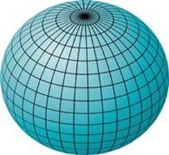
FIGURE 8.1 Longitude and Latitude Lines. Source: http://commons.wikimedia.org/wiki/Image:Sphere_filled_blue.svg rights, GNU Free Documentation license, Creative Commons Attribution ShareAlike license.

Longitude was harder and required accurate clocks for the best and simplest solution. You set a clock to Greenwich Mean Time, take the local solar time, and directly compute the longitude. But clocks were not accurate and did not travel well on ships. A functional clock was finally built in the 1770 s by John Harrison, a Yorkshire carpenter. The previous method was the lunar distance method, which required lookup tables, the sun, the moon, and ten stars to find longitude at sea, but it was accurate to within half a degree. Since these tables were based on the Royal Observatory, Greenwich Mean Time became the international standard.

Most GIS problems are local enough to pretend that the Earth is flat. This avoids spherical trigonometry and puts us back into plane geometry. Hooray! We can draw maps from survey data and we are more worried about polygons and lines that represent neighborhoods, political districts, roads, and other human-made geographical features.

Unfortunately, these things were not that well measured in the past. In Texas and other larger western states, the property lines were surveyed 200 or more years ago (much of it done by the Spanish/Mexican period) with the equipment available at that time. Many of the early surveys used physical features that have moved; rivers are the most common example, but survey markers have also been lost or moved. Texas is big, so a small error in an angle or a boundary marker becomes a narrow wedge shape of no-man’s land between property lines. These wedges and overlaps are very large in parts of west Texas. They also become overlapping property boundaries.

But do not think that having modern GPS will prevent errors. They also have errors, though much fewer and smaller than traditional survey tools produce. Two receivers at adjacent locations often experience similar errors, but they can often be corrected statistically. The difference in coordinates between the two receivers should be significantly more accurate than the absolute position of each receiver; this is called differential positioning. GPS can be blocked by physical objects and we are not talking about big objects. Mesh fences or other small objects can deflect the satellite signal. Multipath errors occur when the satellite signal takes two routes to the receiver. Then we have atmospheric disturbances that do to GPSs what they do to your television satellite dish reception.

These surveys need to be redone. We have the technology today to establish the borders and corners of the polygon that define a parcel of land far better than we did even ten years ago. But there are legal problems concerning who would get title to the thousands of acres in question and what jurisdictions the amended property would belong to. If you want to get more information, look at the types of land surveys at http://hovell.net/types.htm.

8.2.2 Hierarchical Triangular Mesh

An alternative to (longitude, latitude) pairs is the hierarchical triangular mesh (HTM). While (longitude, latitude) pairs are based on establishing a point in a two-dimensional coordinate system on the surface of the Earth, HTM is based on dividing the surface into almost-equal-size triangles with a unique identifier to locate something by a containing polygon. The HTM index is superior to cartographical methods using coordinates with singularities at the poles.

If you have seen a geodesic dome or Buckminster Fuller’s map, you have some feeling for this approach. HTM starts with an octahedron at level zero. To map the globe into an octahedron (regular polyhedron of eight triangles), align it so that the world is first cut into a northern and southern hemisphere. Now slice it along the prime meridian, and then at right angles to both those cuts. In each hemisphere, number the spherical triangles from 0 to 3, with either “N” or “S” in the prefix.

A triangle on a plane always has exactly 180°, but on the surface of a sphere and other positively curved surfaces, it is always greater than 180°, and less than 180° on negatively curved surfaces. If you want a quick mind tool, think that a positively curved surface has too much in the middle. A negatively curved surface is like a horse saddle or the bell of a trumpet; the middle of the surface is too small and curves the shape.

The eight spherical triangles are labeled N0 to N3 and S0 to S3 and are called “level 0 trixels” in the system. Each trixel can be split into four smaller trixels recursively. Put a point at the middle of each edge of the triangle. Use those three points to make an embedded triangle with great circle arc segments. This will divide the original triangle into four more spherical triangles at the next level down. Trixel division is recursive and smaller and smaller trixels to any level you desire (Figures 8.2–8.4).

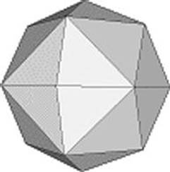
FIGURE 8.2 Second Level Tessellation.

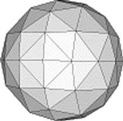
FIGURE 8.3 Third Level Tessellation.

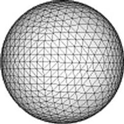
FIGURE 8.4 High Level Tessellation.

To name the new trixels, take the name of the patent trixel and append a digit from 0 to 3 to it, using a counterclockwise pattern. The (n = {0, 1, 2}) point on the corner of the next level is opposite the same number on the corner of the previous level. The center triangle always gets a 3.

The triangles are close to the same size at each level. As they get smaller, the difference also decreases. At level 7 approximately three-quarters of the trixels are slightly smaller than the average size, and one-quarter are larger. The difference is because the three corner trixels (0, 1, 2) are smaller than trixel 3 in the center one. Remember that geometry lesson about triangles on spheres at the start of this section? The ratio of the maximum over the minimum areas at higher depths is about two. Obviously, smaller trixels have longer names and the length of the name gives its level.

The name can be used to compute the exact location of the three vertex vectors of the given trixel. They can be easily encoded into an integer identifier by assigning 2 bits to each level and encoding “N” as 11 and “S” as 10. For example, N01 encodes as binary 110001 or hexadecimal 0x31. The HTM ID (HtmID) is the number of a trixel (and its center point) as a unique 64-bit string (not all strings are valid trixels).

While the recursion can go to infinite, the smallest valid HtmID is 8 levels but it is easy to go to 31 levels, represented in 64 bits. Level 25 is good enough for most applications, since it is about 0.6 meters on the surface of the Earth or 0.02 arc-seconds. Level 26 is about 30 centimeters (less than one foot) on the Earth’s surface. If you want to get any closer than that to an object, you are probably trying to put a bullet in it or perform surgery.

The tricky stuff is covering an irregular polygon with trixels. A trixel can be completely inside a region, completely outside a region, overlapping the region, or touching another trixel. Obviously, the smaller the trixels used to approximate the region, the closer the approximation of the area. If we assume that the location of something is in the center of a trixel, then we can do some math or build a lookup table to get the distance between locations. Beyond depth 7, the curvature of the Earth becomes irrelevant, so distances within a trixel are simple Cartesian calculations. You spread the triangle out flat and run a string between the departure and destination triangles. You can get more math than you probably want in Microsoft research paper MSR-TR-2005-123.

8.2.3 Street Addresses

The United States and many other counties are moving to what we call the nine-one-one system. It assigns a street address that has a known (longitude, latitude) that can be used by emergency services, hence the name. Before this, an address like “The Johnson Ranch” was used in rural areas.

A database known as the Master Street Address Guide (MSAG) describes address elements, including the exact spellings of street names and street number ranges. It ties into the U.S. Postal Service’s (USPS) Coding Accuracy Support System (CASS). You can get the basic details of CASS at http://pe.usps.com/text/pub28.

The use of U.S.-style addresses is not universal. In Korea, a big debate was started in 2012 when the country switched from the Japanese system to the U.S. system. In the Japanese system, a town or city is divided into neighborhoods. Within each neighborhood, streets have local names and the buildings are numbered in the order they were built. Numbers are not reused when a building is destroyed. There is no way to navigate in such a system unless you already know where something is. There is no way to get geographical data from these addresses.

The objection in Korea came from Buddhist groups. Many of the neighborhoods were named after Buddhist saints and they were afraid those names would disappear when physically contiguous streets were give a uniform name.

8.2.4 Postal Codes

I cannot review all of the postal addresses on Earth. Showing a cultural basis, I will look at the United States, Canada, and the United Kingdom. They are all English-speaking nations with a common heritage, so you might expect some commonality. Wrong again.

Postal codes can be broadly lumped into those based on geography and those based on the postal delivery system. The U.S. ZIP code system is highly geographical, the Canadian system is less so, and the U.K. system is based on the post offices in the 1800 s.

8.2.5 ZIP Codes

The zone improvement plan (ZIP) code is a postal code system used by the USPS. The term ZIP code was a registered servicemark (a type of trademark) held by the USPS, but the registration expired. Today the term has become almost a generic name for any postal code, and almost nobody remembers what it originally meant. The basic format is a string of five digits that appear after the state abbreviation code in a U.S. address. An extended ZIP + 4 code was introduced in 1983, which includes the five digits of the ZIP code, a hyphen, and four more digits that determine a more precise location than the ZIP code alone.

The code is based on geography, which means that locations with the same ZIP code are physically contiguous. The first digit is a contiguous group of states.

The first three digits identify the sectional center facility (SCF). An SCF sorts and dispatches mail to all post offices with those first three digits in their ZIP codes. Most of the time, this aligns with state borders, but there are some exceptions for military bases and other locations that cross political units or that can be best served by a closer SCF.

The last two digits are an area within the SCF. But this does not have to match to a political boundary. They tend to identify a local post office or station that serves a given area.

8.2.6 Canadian Postal Codes

Canada (www.canadapost.ca) was one of the last western countries to get a nationwide postal code system (1971). A Canadian postal code is a string of six characters that forms part of a postal address in Canada. This is an example of an alphanumeric system that has less of a geographical basis than the ZIP codes used in the United States. The format is

postal_code SIMILAR TO '[:UPPER:][:DIGIT:][:UPPER:] [:DIGIT:] [:UPPER:][:DIGIT:]'

Notice the space separating the third and fourth characters. The first three characters are a forward sortation area (FSA), which is geographical—for example, A0A is in Newfoundland and Y1A in the Yukon.

But this is not a good validation. The letters D, F, I, O, Q, and U are not allowed because handwritten addresses might make them look like digits or other letters when they are scanned. The letters W and Z are not used as the first letter. The first letter of an FSA code denotes a particular postal district, which, outside of Quebec and Ontario, corresponds to an entire province or territory. Owing to Quebec’s and Ontario’s large populations, those two provinces have three and five postal districts, respectively, and each has at least one urban area so populous that it has a dedicated postal district (“H” for Laval and Montréal, and “M” for Toronto).

At the other extreme, Nunavut and the Northwest Territories (NWT) are so small they share a single postal district. The digit specifies if the FSA is rural (zero) or urban (nonzero). The second letter represents a specific rural region, entire medium-size city, or section of a major metropolitan area.

The last three characters denote a local delivery unit (LDU). An LDU denotes a specific single address or range of addresses, which can correspond to an entire small town, a significant part of a medium-size town, a single side of a city block in larger cities, a single large building or a portion of a very large one, a single large institution such as a university or a hospital, or a business that receives large volumes of mail on a regular basis. LDUs ending in zero are postal facilities, from post offices and small retail postal outlets all the way to sortation centers.

In urban areas, LDUs may be specific postal carriers’ routes. In rural areas where direct door-to-door delivery is not available, an LDU can describe a set of post office boxes or a rural route. LDU 9Z9 is used exclusively for Business Reply Mail. In rural FSAs, the first two characters are usually assigned in alphanumerical order by the name of each community.

LDU 9Z0 refers to large regional distribution center facilities, and is also used as a placeholder, appearing in some regional postmarks such as K0H 9Z0 on purely local mail within the Kingston, Ontario, area.

8.2.7 Postcodes in the United Kingdom

These codes were introduced by the Royal Mail over a 15-year period from 1959 to 1974 and are defined in part by British Standard BS-7666 rules. Strangely enough they are also the lowest level of aggregation in census enumeration. U.K. postcodes are variable-length alphanumeric, making them hard to computerize. The format does not work well for identifying the main sorting office and suboffice. They seem to have been based on what the Royal Post looked like several decades or centuries ago by abbreviating local names at various times in the 15-year period they began.

Postcodes have been supplemented by a newer system of five-digit codes called Mailsort, but only for bulk mailings of 4,000 or more letter-size items. Bulk mailers who use the Mailsort system get a discount, but bulk deliveries by postcode do not.

Postcode Formats

The format of U.K. postcode is generally given by the regular expression:

(GIR 0AA|[A-PR-UWYZ]([0-9]{1,2}|([A-HK-Y][0-9]|[A-HK-Y][0-9]([0-9]| [ABEHMNPRV-Y]))|[0-9][A-HJKS-UW]) [0-9][ABD-HJLNP-UW-Z]{2})

It is broken into two parts with a space between them. It is a hierarchical system, working from left to right—the first letter or pair of letters represents the area, the following digit or digits represents the district within that area, and so on. Each postcode generally represents a street, part of a street, or a single address. This feature makes the postcode useful to route planning software.

The part before the space is the outward code, which identifies the destination sorting office. The outward code can be split further into the area part (letters identifying one of 124 postal areas) and the district part (usually numbers); the letters in the inward code exclude C, I, K, M, O, and V to avoid confusing scanners. The letters of the outward code approximate an abbreviation of the location (London breaks this pattern). For example, “L” is Liverpool, “EH” is Edinburgh, “AB” is Aberdeen, and “BT” is Belfast and all of Northern Ireland.

The remaining part is the inward code, which is used to sort the mail into local delivery routes. The inward code is split into the sector part (one digit) and the unit part (two letters). Each postcode identifies the address to within 100 properties (with an average of 15 properties per postcode), although a large business may have a single code.

Greater London Postcodes

In London, postal area postcodes are based on the 1856 system of postal districts. They do not match the current boundaries of the London boroughs and can overlap into counties in the greater London area. The numbering system appears arbitrary on the map because it is historical rather than geographical.

The most central London areas needed more postcodes than were possible in an orderly pattern, so they have codes like EC1A 1AA to make up the shortage. Then some codes are constructed by the government for their use, without regard to keeping a pattern. For example, in Westminster:

◆ SW1A 0AA: House of Commons

◆ SW1A 0PW: House of Lords, Palace of Westminster

◆ SW1A 1AA: Buckingham Palace

◆ SW1A 2AA: 10 Downing Street, Prime Minister and First Lord of the Treasury

◆ SW1A 2AB: 11 Downing Street, Chancellor of the Exchequer

◆ SW1A 2HQ: HM Treasury headquarters

◆ W1A 1AA: Broadcasting House

◆ W1A 1AB: Selfridges

◆ N81 1ER: Electoral Reform Society has all of N81

There are also nongeographic postcodes, such as outward code BX, so that they can be retained if the recipient changes physical locations. Outward codes beginning XY are used internally for misaddressed mail and international outbound mail. This does not cover special postcodes for the old Girobank, Northern Ireland, Crown dependencies, British Forces Post Office (BFPO), and overseas territories.

In short, the system is so complex that you require software and data files from the Royal Post (postcode address file, or PAF, which has about 27 million U.K. commercial and residential addresses) and specialized software. The PAF is not given out free by the Royal Mail, but licensed for commercial use by software vendors and updated monthly. In the United Kingdom, most addresses can be constructed from just the postcode and a house number. But not in an obvious way, so GISs have to depend on lookup files to translate the address into geographical locations.

8.3 SQL Extensions for GIS

In 1991, the National Institute for Science and Technology (NIST) set up the GIS/SQL work group to look at GIS extensions. Their work is available as “Towards SQL Database Language Extensions for Geographic Information Systems” at http://books.google.com.

In 1997, the Open Geospatial Consortium (OGC) published “OpenGIS Simple Features Specifications for SQL,” which proposes several conceptual ways for extending SQL to support spatial data. This specification is available from the OGC website athttp://www.opengis.org/docs/99-049.pdf. For example, PostGIS is an open-source, freely available, and fairly OGC-compliant spatial database extender for the PostgreSQL Database Management System. SQL Server 2008 has its spatial support: there is Oracle Spatial, and the DB2 spatial extender. These extensions add spatial functions such as distance, area, union, intersection, and specialty geometry data types to the database, using the OGC standards.

The bad news is that they all have the feeling of an OO add-on stuck to the side of the RDBMS model. The simple truth is that GIS is different from RDBMS. The best user interface for GIS is graphical, while RDBMS works best with the linear programming language Dr. Codd required in his famous 12 rules.

Concluding Thoughts

The advent of Internet maps (MapQuest, Google Maps, etc.) and personal GPS on cellphones has made “the man on the street” (pun intended) aware of GIS as a type of everyday data. Touch screens also have made it easy to use a GIS system on portable devices. But this hides the more complex uses that are possible when traditional data is put in a GIS database.

References

1. Gray, J. (2004). Szalay, A. S.; Fekete, G.; Mullane, W. O.; Nieto-Santisteban, M. A.; Thakar, A.R., Heber, G.; Rots, A. H.; MSR-TR-2004-32, There goes the neighborhood: Relational algebra for spatial data search. http://research.microsoft.com/pubs/64550/tr-2004-32.pdf.

2. Open Geospatial Consortium. OpenGIS simple features specifications for SQL. 1997; In: http://www.opengis.org/docs/99-049.pdf; 1997.

3. Picquet C. Rapport sur la marche et les effets du choléra dans Paris et Le Département de la Seine. 1832; In: http://gallica.bnf.fr/ark:/12148/bpt6k842918; 1832.

4. Szalay, A. (2005). Gray, J.; Fekete, G.; Kunszt, P.; Kukol, P. & Thakar A. MSR-TR-2005-123, Indexing the sphere with the hierarchical triangular mesh. http://research.microsoft.com/apps/pubs/default.aspx?id=64531.