R Recipes: A Problem-Solution Approach (2014)

Chapter 1. Migrating to R: As Easy As 1, 2, 3

There are compelling reasons to use R. An enthusiastic community of users, programmers, and contributors support R and its evolution. R is accurate, produces excellent graphs, has a variety of built-in functions, and is both a functional language and an object-oriented one. R is completely free and is distributed as open-source software. Here is how to get started. It really is as easy as 1, 2, 3.

Getting R Up and Running on Your System

The current version at the time of this writing was R 3.1.0. A recent version needs to be available on your computer in order for you to benefit from the R recipes you will learn in this book. Many users migrate to R from other statistical packages, while other users migrate to R from other programming languages. Both types of users are in for a bit of a shock. R is a programming language, but very much unlike most other ones. R is not exactly a statistics package, but rather an environment that includes many traditional statistical analyses. This is neither a statistics book nor an R programming book, though we will cover elements of both when solving problems within the recipes contained in this book.

Visit the Comprehensive R Archive Network (http://cran.us.r-project.org/); see the screen capture in Figure 1-1. Users of PCs and Macs can download precompiled binary files, whereas Linux users may have to do the compiling on their own. However, many Linux systems have R as part of their distributions, so Linux users may already have R preinstalled (I’ll show you how to check this later in this section).

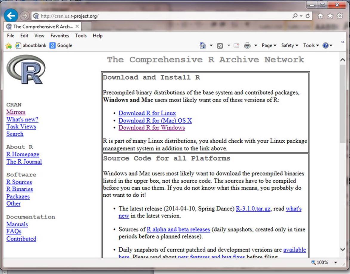
Figure 1-1. The Comprehensive R Archive Network

Click Mirrors and select the site closest to you. Download the precompiled binary files for your system or follow the instructions for compiling the source code if you need to do so. If you have never installed R, install the base distribution first. Most users of Windows will be able to use the 32-bit version of R. If you want to explore the advantages and disadvantages of using the 64-bit version (assuming you have a 64-bit Windows system), look at the information provided by the R Project to help you choose. You can also do what I did, and install both the 32-bit and the 64-bit versions.

Choose your installation language and options. The defaults are fine for most users. If the R installation was successful, you will have a directory labeled R and a desktop icon for launching R. Figure 1-2 shows the opening screen of R 3.1.0 in a Windows 7 environment.

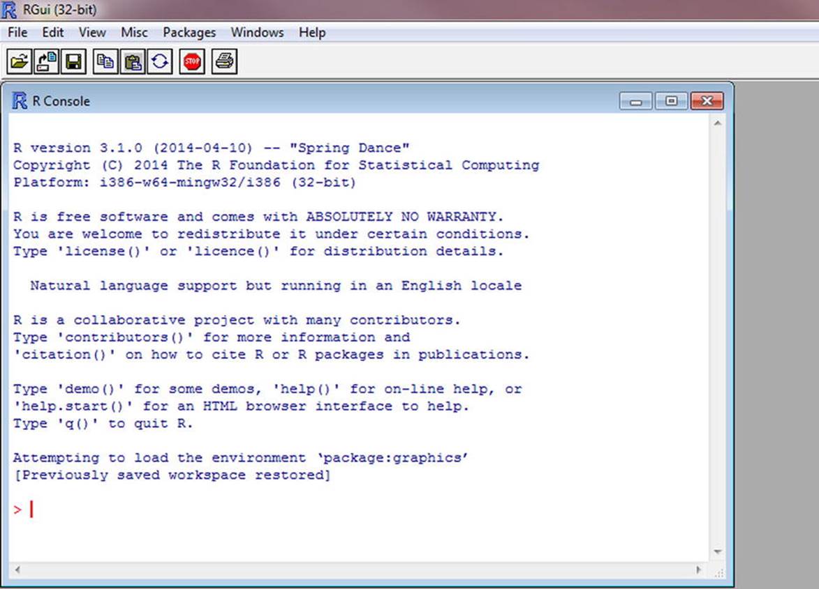
Figure 1-2. The R Console appears in the R GUI

As I mentioned, Linux users may have to compile the R source code, but should first check to see if R is distributed with their version of Linux. For instance, I use Lubuntu, a distribution of Linux, on one of my computers, and the base version of R comes prepackaged with Lubuntu, as it does with most Ubuntu versions. To see if you have R base in your Linux system, use the following commands. Open a terminal session. The command prompt in Linux is the tilde character (~) followed by the dollar sign ($).

~$: sudo apt-get install r-base

Once you have installed the base version of R, you can run R from the terminal as follows:

~$: R

Note that the Linux version of R is not likely to be the latest one, as I am currently running R 3.0.2 in Linux (see Figure 1-3) .

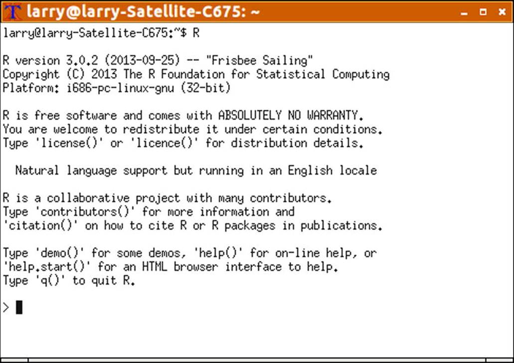
Figure 1-3. R running in a Linux system (Lubuntu)

As you see in Figures 1-2 and 1-3, the command prompt in R is >. The following section will show you how to take R for a quick spin.

Okay, So I Have R. What’s Next?

Whether you are a programmer or a statistician, or like me, a little of both, R takes some getting used to. Most statistics programs, such as SPSS, separate the data, the syntax (programming language), and the output. R takes a minimalist stance on this. If you are not using something, it is not visible to you. If you need to use something, either you must open it, as in the R Editor for writing and saving R scripts, or R will open it for you, as in the R Graphics Device when you generate a histogram or some other graphic output. So, let’s see how to get around in the R interface.

A quick glance shows that the R interface is not particularly fancy, but it is highly functional. Examine the options available to you in the menu bar and the icon bar. R opens with the welcome screen shown in Figure 1-2. You can keep that if you like (I like it), or simply press Ctrl+L or select Edit Clear Console to clear the console. You will be working in the R Console most of the time, but you can open a window with a simple text editor for writing scripts and functions. Do this by selecting File New script. The built-in R Editor is convenient for writing longer scripts and functions, but also simply for writing R commands and editing them before you run them. Many R users prefer to use the text editor of their liking. For Windows users, Notepad is fine. When you produce a graphic object, the R Graphics Device will open. The R GUI (graphical user interface) is completely customizable as well.

Although we are showing R running in the R Console, you should be aware that there are several integrated development environments (IDEs) for R. One of the best of these is RStudio.

Do not worry about losing your output when you clear the console. This is simply the view of what you have on the screen at the moment. The output will scroll off the window when you type other commands and generate new output. Your complete R session is saved to a history file, and you can save and reload your R workspaces. The obvious advantage of saving your workspace is that you do not have to reload the data and functions you used in your R session. Everything will be there again when you reload the workspace.

You will most likely not be interested in saving your R workspace with the examples from this chapter. If you do want to save an R workspace, you will receive a prompt when you quit the session. To exit the session, enter q() or select File Exit. R will give you the prompt shown inFigure 1-4.

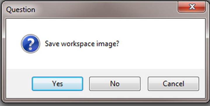
Figure 1-4. R prompts the user to save the workspace image

From this point forward, the R Console is shown only in special cases. The R commands and output will always appear in code font, as explained in the introduction. Launch R if it is not already running on your system. The best way to learn from this book is to have R running and to try to duplicate the screens you see in the book. If you can do that, you will learn a great deal about using R for data analysis and statistics.

First, we will do some simple math, and then we will do some more interesting and a little more complicated things. In R, one assigns values to objects with the assignment operator. The traditional assignment operator is <-. There is also a little-used right-pointing assignment operator, ->. You can also use the equals sign for assignments. There is some advantage in that you avoid two keystrokes when you use = instead of <-. In this book, we will always use <- for assignments. The = sign is used to specify values for arguments and options in R commands. To test for equality, use ==.

R accepts numbers, characters, variables, and even other functions as input to its functions. R is unlike other languages in several important ways. In most computer languages, a number can be assigned to a constant, usually with an equal sign, =. For example, in Python, you can make the assignment x = 10. The value of 10 is assigned to the variable x. The “type” of x is a scalar quantity (a single value) stored as an integer:

Python 3.3.1 (v3.3.1:d9893d13c628, Apr 6 2013, 20:25:12) [MSC v.1600 32 bit (Intel)] on win32
Type "copyright", "credits" or "license()" for more information>>> x = 10
>>> x
10
>>> type(x)
<class 'int'>

If you will remember some of your mathematical or computer training, recall that numerical data can be scalars (individual values or constants), arrays (or vectors) with one row or one column of numbers, or matrices with two or more rows and two or more columns. Many computer languages make distinctions among these data types. In some languages, which are called “strongly typed,” you must declare the variable’s type and dimensionality before you assign a value or values to it. In other languages, known as “loosely typed,” You can assign different types of values to the same variable without having to declare the type. R works that way, and is a very loosely typed language.

To R, there are no scalar quantities. When you enter 1 + 1 and then press Enter, R displays [1] 2 on the next line and gives you another command prompt. The index [1] indicates that to R, the integer object 2 is an integer vector of length 1. The number 2 is the first (and only) element in that vector. You can assign an R command to a variable (object), say, x, and R will keep that assignment until you change it. When we assign x <- 1 + 1, the value of 2 is assigned to the object x. We can now use x in R commands, such as x + 1. R’s indexes start with 1 instead of 0, as some other computer languages do. If you type numbers <- 1:10, R will assign the numbers 1 through 10 to the integer vector called numbers.

> 1 + 1
[1] 2
> x <- 1 + 1
> x + 1
[1] 3
> x * x
[1] 4
> numbers <- 1:10
> numbers
[1] 1 2 3 4 5 6 7 8 9 10
> numbers ^ 2
[1] 1 4 9 16 25 36 49 64 81 100
> numbers * x
[1] 2 4 6 8 10 12 14 16 18 20
> sqrt(numbers)
[1] 1.000000 1.414214 1.732051 2.000000 2.236068 2.449490 2.645751 2.828427
[9] 3.000000 3.162278

As mentioned at the beginning of this chapter, R is both functional and object-oriented. To R, everything is a function, including the basic mathematics operators. Everything is also an object in R. When you assign x <- 1 + 1, you have created an object called x. One of the most useful and powerful features of R is that many of its operators and functions are vectorized

In computer science, something is vectorized if the program works on the vector in elementwise fashion, performing the same operation on each element of the vector that it would have performed on a scalar until it reaches the end of the vector. The general category of array-programming languages includes languages that generalize operations on scalars transparently to vectors, matrices, and higher-order arrays. An operation that works on an entire array is called a vectorized operation. Most computer languages are not vectorized to the extent R is. This makes it easy in many situations to avoid explicit loops, which are very slow in comparison to a vectorized operation. If you work in a scientific or engineering setting, you are probably familiar with MATLAB and Octave. Along with R and Python using the NumPy extension, these languages support array programming.

The only other computer language I have worked with that has the same level of vectorization is the now defunct language APL. In most languages, you would have to write a loop to square the numbers from 1 to 10. But in R, you simply use the exponent operator (^) to square all the numbers at once. The primary advantage of this is that you can frequently avoid explicit loops, as mentioned earlier.

R is case sensitive. Note that x and X are different objects in R. Although R is case sensitive, it is insensitive to spaces. I write code that uses spaces and indentation simply to make it easier for me and others to understand, and I usually comment my code fairly liberally. You would be surprised how often you can be doing something that makes perfectly good sense at the time, but looks like total gibberish when you return to it a few months later. Comments help. To insert a comment in a line of R code, simply enter #. The interpreter ignores anything after the # (pound sign or hash tag).

Here’s a demonstration of the case sensitivity of R and the use of comments. Instead of working directly in the R GUI, click File New Script to open the R Editor. It is far easier to write and correct multiple lines of code in the editor (or in some other text editor) and execute the code from there than to type directly into the R Console. When you work in the R Editor, leave out the > command prompt. R will supply it (see Figure 1-5).

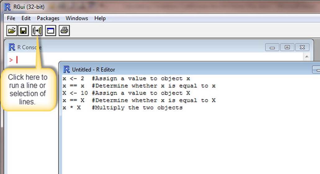
Figure 1-5. Use the R Editor to write multiple lines of R code

To execute your code, select one or more lines of code from the R Editor, and then click the icon for running the code in the R Console. As a shortcut, if you want to run all the code, use Ctrl+A to select all the code, and then press Ctrl+R to run the code in the R Console. Here is what you get:

> x <- 2 #Assign a value to object x
> x == x #Determine whether x is equal to x
[1] TRUE
> X <- 10 #Assign a value to object X
> x == X #Determine whether x is equal to X
[1] FALSE
> x * X #Multiply the two objects
[1] 20
>

Table 1-1 presents some useful operators, functions, and constants in R.

Table 1-1. Useful Operator, Functions, and Constants in R

Table 1-2 shows R’s comparison operators. They evaluate to a logical value of TRUE or FALSE.

Table 1-2. R Comparison Operators

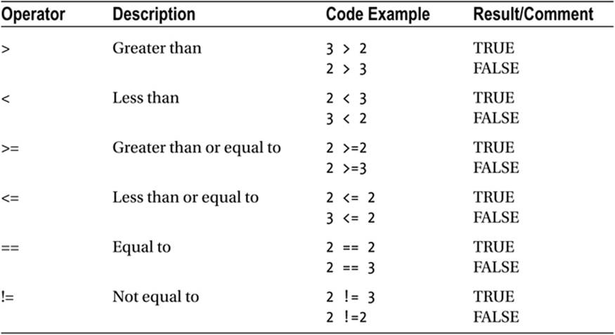
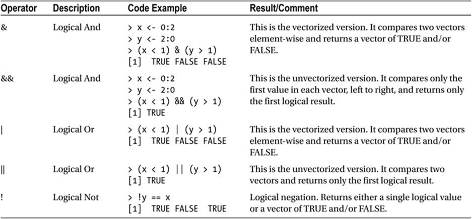
Table 1-3 shows R’s logical operators.

Table 1-3. Logical Operators in R

Understanding the Data Types in R

As the preceding discussion has shown, R is strange in several ways. Remember R is both functional and object-oriented, so it has a bit of an identity crisis when it comes to dealing with data. Instead of the expected integer, floating point, array, and matrix types for expressing numerical values, R uses vectors for all these types of data. Beginning users of R are quickly lost in a swamp of objects, names, classes, and types. The best thing to do is to take the time to learn the various data types in R, and to learn how they are similar to, and often very different from, the ways you have worked with data using other languages or systems.

R has six “atomic” vector types, including logical, integer, real, complex, string (or character) and raw. Another data type in R is the list. Vectors must contain only one type of data, but lists can contain any combination of data types. A data frame is a special kind of list and the most common data object for statistical analysis. Like any list, a data frame can contain both numerical and character information. Some character information can be used for factors, and when that is the case, the data type becomes numeric. Working with factors can be a bit tricky because they are “like” vectors to some extent, but are not exactly vectors. My friends who are programmers think factors are “evil,” while statisticians like me love the fact that verbal labels can be used as factors in R, because such factors are self-labelling. It makes infinitely more sense to have a column in a data frame labelled sex with two entries, male and female, than it does to have a column labelled sex with 0s and 1s in the data frame.

In addition to vectors, lists, and data frames, R has language objects including calls, expressions, and names. There are symbol objects and function objects, as well as expression objects. There is also a special object called NULL, which is used to indicate that an object is absent. Missing data in R are indicated by NA.

We next discuss handling missing data. Then we will touch very briefly on vectors and matrices in R.

Handling Missing Data in R

Create a simple vector using the c() function (some people say it means combine, while others say it means concatenate). I prefer “combine” because there is also a cat() function for concatenating output. For now, just type in the following and observe the results. The na.rm = TRUEoption does not remove the missing value, but simply omits it from the calculations.

> x <- c(10, NA, 10, 25, 30, 15, 10, 18, 16, 15)
> x
[1] 10 NA 10 25 30 15 10 18 16 15
> mean(x)
[1] NA
> mean(x, na.rm = TRUE)
[1] 16.55556
>

Working with Vectors in R

As you have learned, R treats a single number as a vector of length 1. If you create a vector of two or more objects, the vector must contain only a single data type. If you try to make a vector with multiple data types, R will coerce the vector into a single type. Chapter 3 covers how to deal with various data structure in more detail. For now, the goal is simply to show how R works with vectors.

Because you know how to use the R Editor and the R Console now, we will dispense with those formalities and just show the code and the output together. First, we will make a vector of 10 numbers, and then add a character element to the vector. R coerces the data to a character vector because we added a character object to it. I used the index [11] to add another element to the vector. But the vector now does not contain numbers and you cannot do math on it. Use a negative index, [-11], to remove the character and the R function as.integer() to change the vector back to integers:

> x <- 1:10
> x
[1] 1 2 3 4 5 6 7 8 9 10
> typeof(x)
[1] "integer"
> x[11] <- "happy"
> x
[1] "1" "2" "3" "4" "5" "6" "7" "8" "9"
[10] "10" "happy"
> typeof(x)
[1] "character"
> x <- x[-11]
> x
[1] "1" "2" "3" "4" "5" "6" "7" "8" "9" "10"
> x <- as.integer(x)
> x
[1] 1 2 3 4 5 6 7 8 9 10
> typeof(x)
[1] "integer"
>

To make the example a little more interesting, let us work with some real data. The following data (thanks to Nat Goodman for the data) represent the ages in weeks of 20 randomly sampled mice from a much larger dataset.

> ages
[1] 10.5714 13.2857 13.5714 16.0000 10.2857 19.5714 20.0000 7.7143 20.5714
[10] 19.2857 14.0000 14.4286 19.7143 18.0000 13.2857 17.2857 5.2857 16.2857
[19] 14.1429 6.0000
> mean(ages)
[1] 14.46428
> typeof(ages)
[1] "double"
> mode(ages)
[1] "numeric"
> class(ages)
[1] "numeric"

R stores numeric values that are not integers in double-precision form. We can access individual elements of a vector with the index or indexes of those elements. Remember that most R functions and operators are vectorized, so that you can calculate the ages of the mice in months by dividing each age by 4. It takes only one line of code (shown in bold), and looping is not necessary.

> ages[1]
[1] 10.5714
> ages[20]
[1] 6
> ages[3:9]
[1] 13.5714 16.0000 10.2857 19.5714 20.0000 7.7143 20.5714
> months <- ages/4
> months
[1] 2.642850 3.321425 3.392850 4.000000 2.571425 4.892850 5.000000 1.928575
[9] 5.142850 4.821425 3.500000 3.607150 4.928575 4.500000 3.321425 4.321425
[17] 1.321425 4.071425 3.535725 1.500000

When you perform operations with vectors of different lengths, R will repeat the values of the shorter vector to match the length of the longer one. This “recycling” is sometimes very helpful as in multiplication by a scalar (vector of length 1), but sometimes produces unexpected results. If the length of the longer vector is a multiple of the shorter vector, this works well. If not, you get strange results like the following:

> x <- 1:2
> y <- 1:10
> z <- 1:3
> y/x
[1] 1 1 3 2 5 3 7 4 9 5
> y/z
[1] 1.0 1.0 1.0 4.0 2.5 2.0 7.0 4.0 3.0 10.0
Warning message:
In y/z : longer object length is not a multiple of shorter object length

Working with Matrices in R

In another peculiarity of R, a matrix is also a vector, but a vector is not a matrix. I know this sounds like doublespeak, but read on for further explanation. A matrix is a vector with dimensions. You can make a vector into a one-dimensional matrix if you need to do so. Matrix operations are a snap in R. In this book, we work with two-dimensional matrices only, but higher-order matrices are possible, too.

We can create a matrix from a vector of numbers. Start with a vector of 50 random standard normal deviates (z scores if you like). R fills the matrix columnwise.

> zscores <- rnorm(50)
> zscores
[1] -1.19615960 0.95960082 0.50725210 -0.37411224 1.42044733 1.69437460
[7] 0.51677914 -0.04810441 -1.28024577 -0.48968148 1.28769546 0.93050145
[13] 0.72614070 -0.19306114 -0.56122938 0.77504861 -0.26756380 -1.11077206
[19] -0.60040090 -0.31920172 1.16802977 1.69736349 0.93134640 -1.15182325
[25] 0.12167256 -1.16038178 1.00415819 0.54469494 1.60231699 -0.11057038
[31] 0.01264523 0.57436245 0.54283138 -0.53045053 0.18115294 1.16062792
[37] 0.63649217 0.59524893 -0.52972220 0.45013366 0.31892391 -0.32371074
[43] 0.89716628 -0.15187155 0.25808226 1.73149549 1.36917698 -0.05803692
[49] 0.44942046 1.07708172

> zmatrix <- matrix(zscores, nrow = 10, ncol = 5)
> zmatrix
[,1] [,2] [,3] [,4] [,5]
[1,] -1.19615960 1.2876955 1.1680298 0.01264523 0.31892391
[2,] 0.95960082 0.9305014 1.6973635 0.57436245 -0.32371074
[3,] 0.50725210 0.7261407 0.9313464 0.54283138 0.89716628
[4,] -0.37411224 -0.1930611 -1.1518232 -0.53045053 -0.15187155
[5,] 1.42044733 -0.5612294 0.1216726 0.18115294 0.25808226
[6,] 1.69437460 0.7750486 -1.1603818 1.16062792 1.73149549
[7,] 0.51677914 -0.2675638 1.0041582 0.63649217 1.36917698
[8,] -0.04810441 -1.1107721 0.5446949 0.59524893 -0.05803692
[9,] -1.28024577 -0.6004009 1.6023170 -0.52972220 0.44942046
[10,] -0.48968148 -0.3192017 -0.1105704 0.45013366 1.07708172
>

Imagine the five columns are students’ standard scores on four quizzes and a final exam. You can specify names for the rows and columns of the matrix as follows:

> rownames(zmatrix)<-c("Jill","Nat","Jane","Tim","Larry","Harry","Barry","Mary","Gary","Eric")
> zmatrix
[,1] [,2] [,3] [,4] [,5]
Jill -1.19615960 1.2876955 1.1680298 0.01264523 0.31892391
Nat 0.95960082 0.9305014 1.6973635 0.57436245 -0.32371074
Jane 0.50725210 0.7261407 0.9313464 0.54283138 0.89716628
Tim -0.37411224 -0.1930611 -1.1518232 -0.53045053 -0.15187155
Larry 1.42044733 -0.5612294 0.1216726 0.18115294 0.25808226
Harry 1.69437460 0.7750486 -1.1603818 1.16062792 1.73149549
Barry 0.51677914 -0.2675638 1.0041582 0.63649217 1.36917698
Mary -0.04810441 -1.1107721 0.5446949 0.59524893 -0.05803692
Gary -1.28024577 -0.6004009 1.6023170 -0.52972220 0.44942046
Eric -0.48968148 -0.3192017 -0.1105704 0.45013366 1.07708172

> colnames(zmatrix) <- c("quiz1","quiz2","quiz3","quiz4","final")
> zmatrix
quiz1 quiz2 quiz3 quiz4 final
Jill -1.19615960 1.2876955 1.1680298 0.01264523 0.31892391
Nat 0.95960082 0.9305014 1.6973635 0.57436245 -0.32371074
Jane 0.50725210 0.7261407 0.9313464 0.54283138 0.89716628
Tim -0.37411224 -0.1930611 -1.1518232 -0.53045053 -0.15187155
Larry 1.42044733 -0.5612294 0.1216726 0.18115294 0.25808226
Harry 1.69437460 0.7750486 -1.1603818 1.16062792 1.73149549
Barry 0.51677914 -0.2675638 1.0041582 0.63649217 1.36917698
Mary -0.04810441 -1.1107721 0.5446949 0.59524893 -0.05803692
Gary -1.28024577 -0.6004009 1.6023170 -0.52972220 0.44942046
Eric -0.48968148 -0.3192017 -0.1105704 0.45013366 1.07708172

Standardized scores are usually reported to two decimal places. Remove some of the extra decimals to make the next part of the code a little less cluttered. Set the number of decimals by using the round() function:

zmatrix <round(zmatrix, digits = 2)
zmatrix
quiz1 quiz2 quiz3 quiz4 final
Jill -1.20 1.29 1.17 0.01 0.32
Nat 0.96 0.z93 1.70 0.57 -0.32
Jane 0.51 0.73 0.93 0.54 0.90
Tim -0.37 -0.19 -1.15 -0.53 -0.15
Larry 1.42 -0.56 0.12 0.18 0.26
Harry 1.69 0.78 -1.16 1.16 1.73
Barry 0.52 -0.27 1.00 0.64 1.37
Mary -0.05 -1.11 0.54 0.60 -0.06
Gary -1.28 -0.60 1.60 -0.53 0.45
Eric -0.49 -0.32 -0.11 0.45 1.08

If you have occasion to fill a matrix rowwise, set the byrow argument to T or TRUE. You can do this as follows.

> y <- matrix(x, nrow = 10, ncol = 10, byrow = TRUE)
> y

[,1] [,2] [,3] [,4] [,5] [,6] [,7] [,8] [,9] [,10]
[1,] 1 2 3 4 5 6 7 8 9 10
[2,] 11 12 13 14 15 16 17 18 19 20
[3,] 21 22 23 24 25 26 27 28 29 30
[4,] 31 32 33 34 35 36 37 38 39 40
[5,] 41 42 43 44 45 46 47 48 49 50
[6,] 51 52 53 54 55 56 57 58 59 60
[7,] 61 62 63 64 65 66 67 68 69 70
[8,] 71 72 73 74 75 76 77 78 79 80
[9,] 81 82 83 84 85 86 87 88 89 90
[10,] 91 92 93 94 95 96 97 98 99 100

R uses two indexes for the elements of a two-dimensional matrix. As with vectors, the indexes must be enclosed in square brackets. A range of values can be specified by use of the colon operator, as in [1:2]. You can also use a comma to indicate a whole row or a whole column of a matrix. Consider the following examples.

> y[,1:5]
[,1] [,2] [,3] [,4] [,5]
[1,] 1 2 3 4 5
[2,] 11 12 13 14 15
[3,] 21 22 23 24 25
[4,] 31 32 33 34 35
[5,] 41 42 43 44 45
[6,] 51 52 53 54 55
[7,] 61 62 63 64 65
[8,] 71 72 73 74 75
[9,] 81 82 83 84 85
[10,] 91 92 93 94 95
> y[1:5,]
[,1] [,2] [,3] [,4] [,5] [,6] [,7] [,8] [,9] [,10]
[1,] 1 2 3 4 5 6 7 8 9 10
[2,] 11 12 13 14 15 16 17 18 19 20
[3,] 21 22 23 24 25 26 27 28 29 30
[4,] 31 32 33 34 35 36 37 38 39 40
[5,] 41 42 43 44 45 46 47 48 49 50
> y[5,5]
[1] 45
> y[10,10]

[1] 100R can do many useful things with matrices. For example, calculate the variance-covariance matrix by using the var() function:

> varcovar <- var(zmatrix)
> varcovar
quiz1 quiz2 quiz3 quiz4 final
quiz1 1.0544544 0.11489111 -0.3285267 0.3838900 0.19691333
quiz2 0.1148911 0.63790667 0.1006644 0.1074422 0.07846222
quiz3 -0.3285267 0.10066444 1.0574489 -0.0665400 -0.19844667
quiz4 0.3838900 0.10744222 -0.0665400 0.2859656 0.20044222
final 0.1969133 0.07846222 -0.1984467 0.2004422 0.47039556

Invert a matrix by using the solve() function:

> inverse <- solve(varcovar)
> inverse
quiz1 quiz2 quiz3 quiz4 final
quiz1 2.23763294 -0.02683957 0.6305501 -3.3937313 0.7799048
quiz2 -0.02683957 1.72182793 -0.2326712 -0.5743348 -0.1293917
quiz3 0.63055010 -0.23267125 1.2358101 -0.9683403 0.7088308
quiz4 -3.39373126 -0.57433478 -0.9683403 10.3613632 -3.3071827
final 0.77990476 -0.12939168 0.7088308 -3.3071827 3.5292487

Do matrix multiplication by using the %*% operator. Just to make things clear, the matrix product of a matrix and its inverse is an identity matrix with 1’s on the diagonal and 0’s in the off-diagonals. Showing the result with fewer decimals makes this more obvious. For some reason, many of my otherwise very bright students do not “get” scientific notation at all.

> identity <- varcovar %*% inverse
> identity
quiz1 quiz2 quiz3 quiz4 final
quiz1 1.000000e+00 5.038152e-18 3.282422e-17 2.602627e-16 5.529431e-18
quiz2 -8.009544e-18 1.000000e+00 -2.323920e-17 1.080679e-16 -4.710858e-17
quiz3 -7.697835e-17 7.521991e-17 1.000000e+00 9.513874e-17 -9.215718e-17
quiz4 1.076477e-16 1.993407e-17 3.182133e-17 1.000000e+00 -4.325967e-17
final -4.770490e-18 -6.986328e-18 -1.832302e-17 1.560167e-16 1.000000e+00

> identity <- round(identity, 2)
> identity
quiz1 quiz2 quiz3 quiz4 final
quiz1 1 0 0 0 0
quiz2 0 1 0 0 0
quiz3 0 0 1 0 0
quiz4 0 0 0 1 0
final 0 0 0 0 1

Looking Backward and Forward

In Chapter 1, you learned three important things: how to get R, how to use R, and how to work with missing data and various types of data in R. These are foundational skills. In Chapter 2, you will learn more about input and output in R. Chapter 3 will fill in the gaps concerning various data structures, returning to vectors and matrices, as well as learning how to work with lists and data frames.