Machine Learning with Spark (2015)
Chapter 10. Real-time Machine Learning with Spark Streaming
So far in this book, we have focused on batch data processing. That is, all our analysis, feature extraction, and model training has been applied to a fixed set of data that does not change. This fits neatly into Spark's core abstraction of RDDs, which are immutable distributed datasets. Once created, the data underlying the RDD does not change, although we might create new RDDs from the original RDD through Spark's transformation and action operators.
Our attention has also been on batch machine learning models where we train a model on a fixed batch of training data that is usually represented as an RDD of feature vectors (and labels, in the case of supervised learning models).
In this chapter, we will:
· Introduce the concept of online learning, where models are trained and updated on new data as it becomes available
· Explore stream processing using Spark Streaming
· See how Spark Streaming fits together with the online learning approach
Online learning
The batch machine learning methods that we have applied in this book focus on processing an existing fixed set of training data. Typically, these techniques are also iterative, and we have performed multiple passes over our training data in order to converge to an optimal model.
By contrast, online learning is based on performing only one sequential pass through the training data in a fully incremental fashion (that is, one training example at a time). After seeing each training example, the model makes a prediction for this example and then receives the true outcome (for example, the label for classification or real target for regression). The idea behind online learning is that the model continually updates as new information is received instead of being retrained periodically in batch training.
In some settings, when data volume is very large or the process that generates the data is changing rapidly, online learning methods can adapt more quickly and in near real time, without needing to be retrained in an expensive batch process.
However, online learning methods do not have to be used in a purely online manner. In fact, we have already seen an example of using an online learning model in the batch setting when we used stochastic gradient descent optimization to train our classification and regression models. SGD updates the model after each training example. However, we still made use of multiple passes over the training data in order to converge to a better result.
In the pure online setting, we do not (or perhaps cannot) make multiple passes over the training data; hence, we need to process each input as it arrives. Online methods also include mini-batch methods where, instead of processing one input at a time, we process a small batch of training data.
Online and batch methods can also be combined in real-world situations. For example, we can periodically retrain our models offline (say, every day) using batch methods. We can then deploy the trained model to production and update it using online methods in real time (that is, during the day, in between batch retraining) to adapt to any changes in the environment.
As we will see in this chapter, the online learning setting can fit neatly into stream processing and the Spark Streaming framework.
Note
See http://en.wikipedia.org/wiki/Online_machine_learning for more details on online machine learning.
Stream processing
Before covering online learning with Spark, we will first explore the basics of stream processing and introduce the Spark Streaming library.
In addition to the core Spark API and functionality, the Spark project contains another major library (in the same way as MLlib is a major project library) called Spark Streaming, which focuses on processing data streams in real time.
A data stream is a continuous sequence of records. Common examples include activity stream data from a web or mobile application, time-stamped log data, transactional data, and event streams from sensor or device networks.
The batch processing approach typically involves saving the data stream to an intermediate storage system (for example, HDFS or a database) and running a batch process on the saved data. In order to generate up-to-date results, the batch process must be run periodically (for example, daily, hourly, or even every few minutes) on the latest data available.
By contrast, the stream-based approach applies processing to the data stream as it is generated. This allows near real-time processing (of the order of a subsecond to a few tenths of a second time frames rather than minutes, hours, days, or even weeks with typical batch processing).
An introduction to Spark Streaming
There are a few different general techniques to deal with stream processing. Two of the most common ones are as follows:
· Treat each record individually and process it as soon as it is seen.
· Combine multiple records into mini-batches. These mini-batches can be delineated either by time or by the number of records in a batch.
Spark Streaming takes the second approach. The core primitive in Spark Streaming is the discretized stream, or DStream. A DStream is a sequence of mini-batches, where each mini-batch is represented as a Spark RDD:
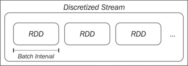
The discretized stream abstraction
A DStream is defined by its input source and a time window called the batch interval. The stream is broken up into time periods equal to the batch interval (beginning from the starting time of the application). Each RDD in the stream will contain the records that are received by the Spark Streaming application during a given batch interval. If no data is present in a given interval, the RDD will simply be empty.
Input sources
Spark Streaming receivers are responsible for receiving data from an input source and converting the raw data into a DStream made up of Spark RDDs.
Spark Streaming supports various input sources, including file-based sources (where the receiver watches for new files arriving at the input location and creates the DStream from the contents read from each new file) and network-based sources (such as receivers that communicate with socket-based sources, the Twitter API stream, Akka actors, or message queues and distributed stream and log transfer frameworks, such Flume, Kafka, and Amazon Kinesis).
Note
See the documentation on input sources at http://spark.apache.org/docs/latest/streaming-programming-guide.html#input-dstreams for more details and for links to various advanced sources.
Transformations
As we saw in Chapter 1, Getting Up and Running with Spark, and throughout this book, Spark allows us to apply powerful transformations to RDDs. As DStreams are made up of RDDs, Spark Streaming provides a set of transformations available on DStreams; these transformations are similar to those available on RDDs. These include map, flatMap, filter, join, and reduceByKey.
Spark Streaming transformations, such as those applicable to RDDs, operate on each element of a DStream's underlying data. That is, the transformations are effectively applied to each RDD in the DStream, which, in turn, applies the transformation to the elements of the RDD.
Spark Streaming also provides operators such as reduce and count. These operators return a DStream made up of a single element (for example, the count value for each batch). Unlike the equivalent operators on RDDs, these do not trigger computation on DStreams directly. That is, they are not actions, but they are still transformations, as they return another DStream.
Keeping track of state
When we were dealing with batch processing of RDDs, keeping and updating a state variable was relatively straightforward. We could start with a certain state (for example, a count or sum of values) and then use broadcast variables or accumulators to update this state in parallel. Usually, we would then use an RDD action to collect the updated state to the driver and, in turn, update the global state.
With DStreams, this is a little more complex, as we need to keep track of states across batches in a fault-tolerant manner. Conveniently, Spark Streaming provides the updateStateByKey function on a DStream of key-value pairs, which takes care of this for us, allowing us to create a stream of arbitrary state information and update it with each batch of data seen. For example, the state could be a global count of the number of times each key has been seen. The state could, thus, represent the number of visits per web page, clicks per advert, tweets per user, or purchases per product, for example.
General transformations
The Spark Streaming API also exposes a general transform function that gives us access to the underlying RDD for each batch in the stream. That is, where the higher level functions such as map transform a DStream to another DStream, transform allows us to apply functions from an RDD to another RDD. For example, we can use the RDD join operator to join each batch of the stream to an existing RDD that we computed separately from our streaming application (perhaps, in Spark or some other system).
Note
The full list of transformations and further information on each of them is provided in the Spark documentation at http://spark.apache.org/docs/latest/streaming-programming-guide.html#transformations-on-dstreams.
Actions
While some of the operators we have seen in Spark Streaming, such as count, are not actions as in the batch RDD case, Spark Streaming has the concept of actions on DStreams. Actions are output operators that, when invoked, trigger computation on the DStream. They are as follows:
· print: This prints the first 10 elements of each batch to the console and is typically used for debugging and testing.
· saveAsObjectFile, saveAsTextFiles, and saveAsHadoopFiles: These functions output each batch to a Hadoop-compatible filesystem with a filename (if applicable) derived from the batch start timestamp.
· forEachRDD: This operator is the most generic and allows us to apply any arbitrary processing to the RDDs within each batch of a DStream. It is used to apply side effects, such as saving data to an external system, printing it for testing, exporting it to a dashboard, and so on.
Tip
Note that like batch processing with Spark, DStream operators are lazy. In the same way in which we need to call an action, such as count, on an RDD to ensure that processing takes place, we need to call one of the preceding action operators in order to trigger computation on a DStream. Otherwise, our streaming application will not actually perform any computation.
Window operators
As Spark Streaming operates on time-ordered batched streams of data, it introduces a new concept, which is that of windowing. A window function computes a transformation over a sliding window applied to the stream.
A window is defined by the length of the window and the sliding interval. For example, with a 10-second window and a 5-second sliding interval, we will compute results every 5 seconds, based on the latest 10 seconds of data in the DStream. For example, we might wish to calculate the top websites by page view numbers over the last 10 seconds and recompute this metric every 5 seconds using a sliding window.
The following figure illustrates a windowed DStream:
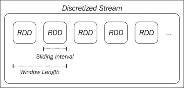
A windowed DStream
Caching and fault tolerance with Spark Streaming
Like Spark RDDs, DStreams can be cached in memory. The use cases for caching are similar to those for RDDs—if we expect to access the data in a DStream multiple times (perhaps performing multiple types of analysis or aggregation or outputting to multiple external systems), we will benefit from caching the data. Stateful operators, which include window functions and updateStateByKey, do this automatically for efficiency.
Recall that RDDs are immutable datasets and are defined by their input data source and lineage—that is, the set of transformations and actions that are applied to the RDD. Fault tolerance in RDDs works by recreating the RDD (or partition of an RDD) that is lost due to the failure of a worker node.
As DStreams are themselves batches of RDDs, they can also be recomputed as required to deal with worker node failure. However, this depends on the input data still being available. If the data source itself is fault-tolerant and persistent (such as HDFS or some other fault-tolerant data store), then the DStream can be recomputed.
If data stream sources are delivered over a network (which is a common case with stream processing), Spark Streaming's default persistence behavior is to replicate data to two worker nodes. This allows network DStreams to be recomputed in the case of failure. Note, however, that any data received by a node but not yet replicated might be lost when a node fails.
Spark Streaming also supports recovery of the driver node in the event of failure. However, currently, for network-based sources, data in the memory of worker nodes will be lost in this case. Hence, Spark Streaming is not fully fault-tolerant in the face of failure of the driver node or application.
Note
See http://spark.apache.org/docs/latest/streaming-programming-guide.html#caching—persistence and http://spark.apache.org/docs/latest/streaming-programming-guide.html#fault-tolerance-properties for more details.
Creating a Spark Streaming application
We will now work through creating our first Spark Streaming application to illustrate some of the basic concepts around Spark Streaming that we introduced earlier.
We will expand on the example applications used in Chapter 1, Getting Up and Running with Spark, where we used a small example dataset of product purchase events. For this example, instead of using a static set of data, we will create a simple producer application that will randomly generate events and send them over a network connection. We will then create a few Spark Streaming consumer applications that will process this event stream.
The sample project for this chapter contains the code you will need. It is called scala-spark-streaming-app. It consists of a Scala SBT project definition file, the example application source code, and a \src\main\resources directory that contains a file called names.csv.
The build.sbt file for the project contains the following project definition:
name := "scala-spark-streaming-app"
version := "1.0"
scalaVersion := "2.10.4"
libraryDependencies += "org.apache.spark" %% "spark-mllib" % "1.1.0"
libraryDependencies += "org.apache.spark" %% "spark-streaming" % "1.1.0"
Note that we added a dependency on Spark MLlib and Spark Streaming, which includes the dependency on the Spark core.
The names.csv file contains a set of 20 randomly generated user names. We will use these names as part of our data generation function in our producer application:
Miguel,Eric,James,Juan,Shawn,James,Doug,Gary,Frank,Janet,Michael,James,Malinda,Mike,Elaine,Kevin,Janet,Richard,Saul,Manuela
The producer application
Our producer needs to create a network connection and generate some random purchase event data to send over this connection. First, we will define our object and main method definition. We will then read the random names from the names.csv resource and create a set of products with prices, from which we will generate our random product events:
/**
* A producer application that generates random "product events", up to 5 per second, and sends them over a
* network connection
*/
object StreamingProducer {
def main(args: Array[String]) {
val random = new Random()
// Maximum number of events per second
val MaxEvents = 6
// Read the list of possible names
val namesResource = this.getClass.getResourceAsStream("/names.csv")
val names = scala.io.Source.fromInputStream(namesResource)
.getLines()
.toList
.head
.split(",")
.toSeq
// Generate a sequence of possible products
val products = Seq(
"iPhone Cover" -> 9.99,
"Headphones" -> 5.49,
"Samsung Galaxy Cover" -> 8.95,
"iPad Cover" -> 7.49
)
Using the list of names and map of product name to price, we will create a function that will randomly pick a product and name from these sources, generating a specified number of product events:
/** Generate a number of random product events */
def generateProductEvents(n: Int) = {
(1 to n).map { i =>
val (product, price) = products(random.nextInt(products.size))
val user = random.shuffle(names).head
(user, product, price)
}
}
Finally, we will create a network socket and set our producer to listen on this socket. As soon as a connection is made (which will come from our consumer streaming application), the producer will start generating random events at a random rate between 0 and 5 per second:
// create a network producer
val listener = new ServerSocket(9999)
println("Listening on port: 9999")
while (true) {
val socket = listener.accept()
new Thread() {
override def run = {
println("Got client connected from: " + socket.getInetAddress)
val out = new PrintWriter(socket.getOutputStream(), true)
while (true) {
Thread.sleep(1000)
val num = random.nextInt(MaxEvents)
val productEvents = generateProductEvents(num)
productEvents.foreach{ event =>
out.write(event.productIterator.mkString(","))
out.write("\n")
}
out.flush()
println(s"Created $num events...")
}
socket.close()
}
}.start()
}
}
}
Note
This producer example is based on the PageViewGenerator example in the Spark Streaming examples.
The producer can be run by changing into the base directory of scala-spark-streaming-app and using SBT to run the application, as we did in Chapter 1, Getting Up and Running with Spark:
>cd scala-spark-streaming-app
>sbt
[info] ...
>
Use the run command to execute the application:
>run
You should see output similar to the following:
...
Multiple main classes detected, select one to run:
[1] StreamingProducer
[2] SimpleStreamingApp
[3] StreamingAnalyticsApp
[4] StreamingStateApp
[5] StreamingModelProducer
[6] SimpleStreamingModel
[7] MonitoringStreamingModel
Enter number:
Select the StreamingProducer option. The application will start running, and you should see the following output:
[info] Running StreamingProducer
Listening on port: 9999
We can see that the producer is listening on port 9999, waiting for our consumer application to connect.
Creating a basic streaming application
Next, we will create our first streaming program. We will simply connect to the producer and print out the contents of each batch. Our streaming code looks like this:
/**
* A simple Spark Streaming app in Scala
*/
object SimpleStreamingApp {
def main(args: Array[String]) {
val ssc = new StreamingContext("local[2]", "First Streaming App", Seconds(10))
val stream = ssc.socketTextStream("localhost", 9999)
// here we simply print out the first few elements of each
// batch
stream.print()
ssc.start()
ssc.awaitTermination()
}
}
It looks fairly simple, and it is mostly due to the fact that Spark Streaming takes care of all the complexity for us. First, we initialized a StreamingContext (which is the streaming equivalent of the SparkContext we have used so far), specifying similar configuration options that are used to create a SparkContext. Notice, however, that here we are required to provide the batch interval, which we set to 10 seconds.
We then created our data stream using a predefined streaming source, socketTextStream, which reads text from a socket host and port and creates a DStream[String]. We then called the print function on the DStream; this function prints out the first few elements of each batch.
Tip
Calling print on a DStream is similar to calling take on an RDD. It displays only the first few elements.
We can run this program using SBT. Open a second terminal window, leaving the producer program running, and run sbt:
>sbt
[info] ...
>run
....
Again, you should see a few options to select:
Multiple main classes detected, select one to run:
[1] StreamingProducer
[2] SimpleStreamingApp
[3] StreamingAnalyticsApp
[4] StreamingStateApp
[5] StreamingModelProducer
[6] SimpleStreamingModel
[7] MonitoringStreamingModel
Run the SimpleStreamingApp main class. You should see the streaming program start up, displaying output similar to the one shown here:
...
14/11/15 21:02:23 INFO scheduler.ReceiverTracker: ReceiverTracker started
14/11/15 21:02:23 INFO dstream.ForEachDStream: metadataCleanupDelay = -1
14/11/15 21:02:23 INFO dstream.SocketInputDStream: metadataCleanupDelay = -1
14/11/15 21:02:23 INFO dstream.SocketInputDStream: Slide time = 10000 ms
14/11/15 21:02:23 INFO dstream.SocketInputDStream: Storage level = StorageLevel(false, false, false, false, 1)
14/11/15 21:02:23 INFO dstream.SocketInputDStream: Checkpoint interval = null
14/11/15 21:02:23 INFO dstream.SocketInputDStream: Remember duration = 10000 ms
14/11/15 21:02:23 INFO dstream.SocketInputDStream: Initialized and validated org.apache.spark.streaming.dstream.SocketInputDStream@ff3436d
14/11/15 21:02:23 INFO dstream.ForEachDStream: Slide time = 10000 ms
14/11/15 21:02:23 INFO dstream.ForEachDStream: Storage level = StorageLevel(false, false, false, false, 1)
14/11/15 21:02:23 INFO dstream.ForEachDStream: Checkpoint interval = null
14/11/15 21:02:23 INFO dstream.ForEachDStream: Remember duration = 10000 ms
14/11/15 21:02:23 INFO dstream.ForEachDStream: Initialized and validated org.apache.spark.streaming.dstream.ForEachDStream@5a10b6e8
14/11/15 21:02:23 INFO scheduler.ReceiverTracker: Starting 1 receivers
14/11/15 21:02:23 INFO spark.SparkContext: Starting job: runJob at ReceiverTracker.scala:275
...
At the same time, you should see that the terminal window running the producer displays something like the following:
...
Got client connected from: /127.0.0.1
Created 2 events...
Created 2 events...
Created 3 events...
Created 1 events...
Created 5 events...
...
After about 10 seconds, which is the time of our streaming batch interval, Spark Streaming will trigger a computation on the stream due to our use of the print operator. This should display the first few events in the batch, which will look something like the following output:
...
14/11/15 21:02:30 INFO spark.SparkContext: Job finished: take at DStream.scala:608, took 0.05596 s
-------------------------------------------
Time: 1416078150000 ms
-------------------------------------------
Michael,Headphones,5.49
Frank,Samsung Galaxy Cover,8.95
Eric,Headphones,5.49
Malinda,iPad Cover,7.49
James,iPhone Cover,9.99
James,Headphones,5.49
Doug,iPhone Cover,9.99
Juan,Headphones,5.49
James,iPhone Cover,9.99
Richard,iPad Cover,7.49
...
Tip
Note that you might see different results, as the producer generates a random number of random events each second.
You can terminate the streaming app by pressing Ctrl + C. If you want to, you can also terminate the producer (if you do, you will need to restart it again before starting the next streaming programs that we will create).
Streaming analytics
Next, we will create a slightly more complex streaming program. In Chapter 1, Getting Up and Running with Spark, we calculated a few metrics on our dataset of product purchases. These included the total number of purchases, the number of unique users, the total revenue, and the most popular product (together with its number of purchases and total revenue).
In this example, we will compute the same metrics on our stream of purchase events. The key difference is that these metrics will be computed per batch and printed out.
We will define our streaming application code here:
/**
* A more complex Streaming app, which computes statistics and prints the results for each batch in a DStream
*/
object StreamingAnalyticsApp {
def main(args: Array[String]) {
val ssc = new StreamingContext("local[2]", "First Streaming App", Seconds(10))
val stream = ssc.socketTextStream("localhost", 9999)
// create stream of events from raw text elements
val events = stream.map { record =>
val event = record.split(",")
(event(0), event(1), event(2))
}
First, we created exactly the same StreamingContext and socket stream as we did earlier. Our next step is to apply a map transformation to the raw text, where each record is a comma-separated string representing the purchase event. The map function splits the text and creates a tuple of (user, product, price). This illustrates the use of map on a DStream and how it is the same as if we had been operating on an RDD.
Next, we will use foreachRDD to apply arbitrary processing on each RDD in the stream to compute our desired metrics and print them to the console:
/*
We compute and print out stats for each batch.
Since each batch is an RDD, we call forEeachRDD on the DStream, and apply the usual RDD functions
we used in Chapter 1.
*/
events.foreachRDD { (rdd, time) =>
val numPurchases = rdd.count()
val uniqueUsers = rdd.map { case (user, _, _) => user }.distinct().count()
val totalRevenue = rdd.map { case (_, _, price) => price.toDouble }.sum()
val productsByPopularity = rdd
.map { case (user, product, price) => (product, 1) }
.reduceByKey(_ + _)
.collect()
.sortBy(-_._2)
val mostPopular = productsByPopularity(0)
val formatter = new SimpleDateFormat
val dateStr = formatter.format(new Date(time.milliseconds))
println(s"== Batch start time: $dateStr ==")
println("Total purchases: " + numPurchases)
println("Unique users: " + uniqueUsers)
println("Total revenue: " + totalRevenue)
println("Most popular product: %s with %d purchases".format(mostPopular._1, mostPopular._2))
}
// start the context
ssc.start()
ssc.awaitTermination()
}
}
If you compare the code operating on the RDDs inside the preceding foreachRDD block with that used in Chapter 1, Getting Up and Running with Spark, you will notice that it is virtually the same code. This shows that we can apply any RDD-related processing we wish within the streaming setting by operating on the underlying RDDs, as well as using the built-in higher level streaming operations.
Let's run the streaming program again by calling sbt run and selecting StreamingAnalyticsApp.
Tip
Remember that you might also need to restart the producer if you previously terminated the program. This should be done before starting the streaming application.
After about 10 seconds, you should see output from the streaming program similar to the following:
...
14/11/15 21:27:30 INFO spark.SparkContext: Job finished: collect at Streaming.scala:125, took 0.071145 s
== Batch start time: 2014/11/15 9:27 PM ==
Total purchases: 16
Unique users: 10
Total revenue: 123.72
Most popular product: iPad Cover with 6 purchases
...
You can again terminate the streaming program using Ctrl + C.
Stateful streaming
As a final example, we will apply the concept of stateful streaming using the updateStateByKey function to compute a global state of revenue and number of purchases per user, which will be updated with new data from each 10-second batch. Our StreamingStateAppapp is shown here:
object StreamingStateApp {
import org.apache.spark.streaming.StreamingContext._
We will first define an updateState function that will compute the new state from the running state value and the new data in the current batch. Our state, in this case, is a tuple of (number of products, revenue) pairs, which we will keep for each user. We will compute the new state given the set of (product, revenue) pairs for the current batch and the accumulated state at the current time.
Notice that we will deal with an Option value for the current state, as it might be empty (which will be the case for the first batch), and we need to define a default value, which we will do using getOrElse as shown here:
def updateState(prices: Seq[(String, Double)], currentTotal: Option[(Int, Double)]) = {
val currentRevenue = prices.map(_._2).sum
val currentNumberPurchases = prices.size
val state = currentTotal.getOrElse((0, 0.0))
Some((currentNumberPurchases + state._1, currentRevenue + state._2))
}
def main(args: Array[String]) {
val ssc = new StreamingContext("local[2]", "First Streaming App", Seconds(10))
// for stateful operations, we need to set a checkpoint
// location
ssc.checkpoint("/tmp/sparkstreaming/")
val stream = ssc.socketTextStream("localhost", 9999)
// create stream of events from raw text elements
val events = stream.map { record =>
val event = record.split(",")
(event(0), event(1), event(2).toDouble)
}
val users = events.map{ case (user, product, price) => (user, (product, price)) }
val revenuePerUser = users.updateStateByKey(updateState)
revenuePerUser.print()
// start the context
ssc.start()
ssc.awaitTermination()
}
}
After applying the same string split transformation we used in our previous example, we called updateStateByKey on our DStream, passing in our defined updateState function. We then printed the results to the console.
Start the streaming example using sbt run and by selecting [4] StreamingStateApp (also restart the producer program if necessary).
After around 10 seconds, you will start to see the first set of state output. We will wait another 10 seconds to see the next set of output. You will see the overall global state being updated:
...
-------------------------------------------
Time: 1416080440000 ms
-------------------------------------------
(Janet,(2,10.98))
(Frank,(1,5.49))
(James,(2,12.98))
(Malinda,(1,9.99))
(Elaine,(3,29.97))
(Gary,(2,12.98))
(Miguel,(3,20.47))
(Saul,(1,5.49))
(Manuela,(2,18.939999999999998))
(Eric,(2,18.939999999999998))
...
-------------------------------------------
Time: 1416080441000 ms
-------------------------------------------
(Janet,(6,34.94))
(Juan,(4,33.92))
(Frank,(2,14.44))
(James,(7,48.93000000000001))
(Malinda,(1,9.99))
(Elaine,(7,61.89))
(Gary,(4,28.46))
(Michael,(1,8.95))
(Richard,(2,16.439999999999998))
(Miguel,(5,35.95))
...
We can see that the number of purchases and revenue totals for each user are added to with each batch of data.
Tip
Now, see if you can adapt this example to use Spark Streaming's window functions. For example, you can compute similar statistics per user over the past minute, sliding every 30 seconds.
Online learning with Spark Streaming
As we have seen, Spark Streaming makes it easy to work with data streams in a way that should be familiar to us from working with RDDs. Using Spark's stream processing primitives combined with the online learning capabilities of MLlib's SGD-based methods, we can create real-time machine learning models that we can update on new data in the stream as it arrives.
Streaming regression
Spark provides a built-in streaming machine learning model in the StreamingLinearAlgorithm class. Currently, only a linear regression implementation is available—StreamingLinearRegressionWithSGD—but future versions will include classification.
The streaming regression model provides two methods for usage:
· trainOn: This takes DStream[LabeledPoint] as its argument. This tells the model to train on every batch in the input DStream. It can be called multiple times to train on different streams.
· predictOn: This also takes DStream[LabeledPoint]. This tells the model to make predictions on the input DStream, returning a new DStream[Double] that contains the model predictions.
Under the hood, the streaming regression model uses foreachRDD and map to accomplish this. It also updates the model variable after each batch and exposes the latest trained model, which allows us to use this model in other applications or save it to an external location.
The streaming regression model can be configured with parameters for step size and number of iterations in the same way as standard batch regression—the model class used is the same. We can also set the initial model weight vector.
When we first start training a model, we can set the initial weights to a zero vector, or a random vector, or perhaps load the latest model from the result of an offline batch process. We can also decide to save the model periodically to an external system and use the latest model state as the starting point (for example, in the case of a restart after a node or application failure).
A simple streaming regression program
To illustrate the use of streaming regression, we will create a simple example similar to the preceding one, which uses simulated data. We will write a producer program that generates random feature vectors and target variables, given a fixed, known weight vector, and writes each training example to a network stream.
Our consumer application will run a streaming regression model, training and then testing on our simulated data stream. Our first example consumer will simply print its predictions to the console.
Creating a streaming data producer
The data producer operates in a manner similar to our product event producer example. Recall from Chapter 5, Building a Classification Model with Spark, that a linear model is a linear combination (or vector dot product) of a weight vector, w, and a feature vector, x(that is, wTx). Our producer will generate synthetic data using a fixed, known weight vector and randomly generated feature vectors. This data fits the linear model formulation exactly, so we will expect our regression model to learn the true weight vector fairly easily.
First, we will set up a maximum number of events per second (say, 100) and the number of features in our feature vector (also 100 in this example):
/**
* A producer application that generates random linear regression data.
*/
object StreamingModelProducer {
import breeze.linalg._
def main(args: Array[String]) {
// Maximum number of events per second
val MaxEvents = 100
val NumFeatures = 100
val random = new Random()
The generateRandomArray function creates an array of the specified size where the entries are randomly generated from a normal distribution. We will use this function initially to generate our known weight vector, w, which will be fixed throughout the life of the producer. We will also create a random intercept value that will also be fixed. The weight vector and intercept will be used to generate each data point in our stream:
/** Function to generate a normally distributed dense vector */
def generateRandomArray(n: Int) = Array.tabulate(n)(_ => random.nextGaussian())
// Generate a fixed random model weight vector
val w = new DenseVector(generateRandomArray(NumFeatures))
val intercept = random.nextGaussian() * 10
We will also need a function to generate a specified number of random data points. Each event is made up of a random feature vector and the target that we get from computing the dot product of our known weight vector with the random feature vector and adding the intercept value:
/** Generate a number of random data events*/
def generateNoisyData(n: Int) = {
(1 to n).map { i =>
val x = new DenseVector(generateRandomArray(NumFeatures))
val y: Double = w.dot(x)
val noisy = y + intercept
(noisy, x)
}
}
Finally, we will use code similar to our previous producer to instantiate a network connection and send a random number of data points (between 0 and 100) in text format over the network each second:
// create a network producer
val listener = new ServerSocket(9999)
println("Listening on port: 9999")
while (true) {
val socket = listener.accept()
new Thread() {
override def run = {
println("Got client connected from: " + socket.getInetAddress)
val out = new PrintWriter(socket.getOutputStream(), true)
while (true) {
Thread.sleep(1000)
val num = random.nextInt(MaxEvents)
val data = generateNoisyData(num)
data.foreach { case (y, x) =>
val xStr = x.data.mkString(",")
val eventStr = s"$y\t$xStr"
out.write(eventStr)
out.write("\n")
}
out.flush()
println(s"Created $num events...")
}
socket.close()
}
}.start()
}
}
}
You can start the producer using sbt run, followed by choosing to execute the StreamingModelProducer main method. This should result in the following output, thus indicating that the producer program is waiting for connections from our streaming regression application:
[info] Running StreamingModelProducer
Listening on port: 9999
Creating a streaming regression model
In the next step in our example, we will create a streaming regression program. The basic layout and setup is the same as our previous streaming analytics examples:
/**
* A simple streaming linear regression that prints out predicted value for each batch
*/
object SimpleStreamingModel {
def main(args: Array[String]) {
val ssc = new StreamingContext("local[2]", "First Streaming App", Seconds(10))
val stream = ssc.socketTextStream("localhost", 9999)
Here, we will set up the number of features to match the records in our input data stream. We will then create a zero vector to use as the initial weight vector of our streaming regression model. Finally, we will select the number of iterations and step size:
val NumFeatures = 100
val zeroVector = DenseVector.zeros[Double](NumFeatures)
val model = new StreamingLinearRegressionWithSGD()
.setInitialWeights(Vectors.dense(zeroVector.data))
.setNumIterations(1)
.setStepSize(0.01)
Next, we will again use the map function to transform the input DStream, where each record is a string representation of our input data, into a LabeledPoint instance that contains the target value and feature vector:
// create a stream of labeled points
val labeledStream = stream.map { event =>
val split = event.split("\t")
val y = split(0).toDouble
val features = split(1).split(",").map(_.toDouble)
LabeledPoint(label = y, features = Vectors.dense(features))
}
The final step is to tell the model to train and test on our transformed DStream and also to print out the first few elements of each batch in the DStream of predicted values:
// train and test model on the stream, and print predictions
// for illustrative purposes
model.trainOn(labeledStream)
model.predictOn(labeledStream).print()
ssc.start()
ssc.awaitTermination()
}
}
Tip
Note that because we are using the same MLlib model classes for streaming as we did for batch processing, we can, if we choose, perform multiple iterations over the training data in each batch (which is just an RDD of LabeledPoint instances).
Here, we will set the number of iterations to 1 to simulate purely online learning. In practice, you can set the number of iterations higher, but note that the training time per batch will go up. If the training time per batch is much higher than the batch interval, the streaming model will start to lag behind the velocity of the data stream.
This can be handled by decreasing the number of iterations, increasing the batch interval, or increasing the parallelism of our streaming program by adding more Spark workers.
Now, we're ready to run SimpleStreamingModel in our second terminal window using sbt run in the same way as we did for the producer (remember to select the correct main method for SBT to execute). Once the streaming program starts running, you should see the following output in the producer console:
Got client connected from: /127.0.0.1
...
Created 10 events...
Created 83 events...
Created 75 events...
...
After about 10 seconds, you should start seeing the model predictions being printed to the streaming application console, similar to those shown here:
14/11/16 14:54:00 INFO StreamingLinearRegressionWithSGD: Model updated at time 1416142440000 ms
14/11/16 14:54:00 INFO StreamingLinearRegressionWithSGD: Current model: weights, [0.05160959387864821,0.05122747155689144,-0.17224086785756998,0.05822993392274008,0.07848094246845688,-0.1298315806501979,0.006059323642394124, ...
...
14/11/16 14:54:00 INFO JobScheduler: Finished job streaming job 1416142440000 ms.0 from job set of time 1416142440000 ms
14/11/16 14:54:00 INFO JobScheduler: Starting job streaming job 1416142440000 ms.1 from job set of time 1416142440000 ms
14/11/16 14:54:00 INFO SparkContext: Starting job: take at DStream.scala:608
14/11/16 14:54:00 INFO DAGScheduler: Got job 3 (take at DStream.scala:608) with 1 output partitions (allowLocal=true)
14/11/16 14:54:00 INFO DAGScheduler: Final stage: Stage 3(take at DStream.scala:608)
14/11/16 14:54:00 INFO DAGScheduler: Parents of final stage: List()
14/11/16 14:54:00 INFO DAGScheduler: Missing parents: List()
14/11/16 14:54:00 INFO DAGScheduler: Computing the requested partition locally
14/11/16 14:54:00 INFO SparkContext: Job finished: take at DStream.scala:608, took 0.014064 s
-------------------------------------------
Time: 1416142440000 ms
-------------------------------------------
-2.0851430248312526
4.609405228401022
2.817934589675725
3.3526557917118813
4.624236379848475
-2.3509098272485156
-0.7228551577759544
2.914231548990703
0.896926579927631
1.1968162940541283
...
Congratulations! You've created your first streaming online learning model!
You can shut down the streaming application (and, optionally, the producer) by pressing Ctrl + C in each terminal window.
Streaming K-means
MLlib also includes a streaming version of K-means clustering; this is called StreamingKMeans. This model is an extension of the mini-batch K-means algorithm where the model is updated with each batch based on a combination between the cluster centers computed from the previous batches and the cluster centers computed for the current batch.
StreamingKMeans supports a forgetfulness parameter alpha (set using the setDecayFactor method); this controls how aggressive the model is in giving weight to newer data. An alpha value of 0 means the model will only use new data, while with an alpha value of 1, all data since the beginning of the streaming application will be used.
We will not cover streaming K-means further here (the Spark documentation at http://spark.apache.org/docs/latest/mllib-clustering.html#streaming-clustering contains further detail and an example). However, perhaps you could try to adapt the preceding streaming regression data producer to generate input data for a StreamingKMeans model. You could also adapt the streaming regression application to use StreamingKMeans.
You can create the clustering data producer by first selecting a number of clusters, K, and then generating each data point by:
· Randomly selecting a cluster index.
· Generating a random vector using specific normal distribution parameters for each cluster. That is, each of the K clusters will have a mean and variance parameter, from which the random vectors will be generated using an approach similar to our precedinggenerateRandomArray function.
In this way, each data point that belongs to the same cluster will be drawn from the same distribution, so our streaming clustering model should be able to learn the correct cluster centers over time.
Online model evaluation
Combining machine learning with Spark Streaming has many potential applications and use cases, including keeping a model or set of models up to date on new training data as it arrives, thus enabling them to adapt quickly to changing situations or contexts.
Another useful application is to track and compare the performance of multiple models in an online manner and, possibly, also perform model selection in real time so that the best performing model is always used to generate predictions on live data.
This can be used to do real-time "A/B testing" of models, or combined with more advanced online selection and learning techniques, such as Bayesian update approaches and bandit algorithms. It can also be used simply to monitor model performance in real time, thus being able to respond or adapt if performance degrades for some reason.
In this section, we will walk through a simple extension to our streaming regression example. In this example, we will compare the evolving error rate of two models with different parameters as they see more and more data in our input stream.
Comparing model performance with Spark Streaming
As we have used a known weight vector and intercept to generate the training data in our producer application, we would expect our model to eventually learn this underlying weight vector (in the absence of random noise, which we do not add for this example).
Therefore, we should see the model's error rate decrease over time, as it sees more and more data. We can also use standard regression error metrics to compare the performance of multiple models.
In this example, we will create two models with different learning rates, training them both on the same data stream. We will then make predictions for each model and measure the mean-squared error (MSE) and root mean-squared error (RMSE) metrics for each batch.
Our new monitored streaming model code is shown here:
/**
* A streaming regression model that compares the model performance of two models, printing out metrics for
* each batch
*/
object MonitoringStreamingModel {
import org.apache.spark.SparkContext._
def main(args: Array[String]) {
val ssc = new StreamingContext("local[2]", "First Streaming App", Seconds(10))
val stream = ssc.socketTextStream("localhost", 9999)
val NumFeatures = 100
val zeroVector = DenseVector.zeros[Double](NumFeatures)
val model1 = new StreamingLinearRegressionWithSGD()
.setInitialWeights(Vectors.dense(zeroVector.data))
.setNumIterations(1)
.setStepSize(0.01)
val model2 = new StreamingLinearRegressionWithSGD()
.setInitialWeights(Vectors.dense(zeroVector.data))
.setNumIterations(1)
.setStepSize(1.0)
// create a stream of labeled points
val labeledStream = stream.map { event =>
val split = event.split("\t")
val y = split(0).toDouble
val features = split(1).split(",").map(_.toDouble)
LabeledPoint(label = y, features = Vectors.dense(features))
}
Note that most of the preceding setup code is the same as our simple streaming model example. However, we created two instances of StreamingLinearRegressionWithSGD: one with a learning rate of 0.01 and one with the learning rate set to 1.0.
Next, we will train each model on our input stream, and using Spark Streaming's transform function, we will create a new DStream that contains the error rates for each model:
// train both models on the same stream
model1.trainOn(labeledStream)
model2.trainOn(labeledStream)
// use transform to create a stream with model error rates
val predsAndTrue = labeledStream.transform { rdd =>
val latest1 = model1.latestModel()
val latest2 = model2.latestModel()
rdd.map { point =>
val pred1 = latest1.predict(point.features)
val pred2 = latest2.predict(point.features)
(pred1 - point.label, pred2 - point.label)
}
}
Finally, we will use foreachRDD to compute the MSE and RMSE metrics for each model and print them to the console:
// print out the MSE and RMSE metrics for each model per batch
predsAndTrue.foreachRDD { (rdd, time) =>
val mse1 = rdd.map { case (err1, err2) => err1 * err1 }.mean()
val rmse1 = math.sqrt(mse1)
val mse2 = rdd.map { case (err1, err2) => err2 * err2 }.mean()
val rmse2 = math.sqrt(mse2)
println(
s"""
|-------------------------------------------
|Time: $time
|-------------------------------------------
""".stripMargin)
println(s"MSE current batch: Model 1: $mse1; Model 2: $mse2")
println(s"RMSE current batch: Model 1: $rmse1; Model 2: $rmse2")
println("...\n")
}
ssc.start()
ssc.awaitTermination()
}
}
If you terminated the producer earlier, start it again by executing sbt run and selecting StreamingModelProducer. Once the producer is running again, in your second terminal window, execute sbt run and choose the main class for MonitoringStreamingModel.
You should see the streaming program startup, and after about 10 seconds, the first batch will be processed, printing output similar to the following:
...
14/11/16 14:56:11 INFO SparkContext: Job finished: mean at StreamingModel.scala:159, took 0.09122 s
-------------------------------------------
Time: 1416142570000 ms
-------------------------------------------
MSE current batch: Model 1: 97.9475827857361; Model 2: 97.9475827857361
RMSE current batch: Model 1: 9.896847113385965; Model 2: 9.896847113385965
...
Since both models start with the same initial weight vector, we see that they both make the same predictions on this first batch and, therefore, have the same error.
If we leave the streaming program running for a few minutes, we should eventually see that one of the models has started converging, leading to a lower and lower error, while the other model has tended to diverge to a poorer model due to the overly high learning rate:
...
14/11/16 14:57:30 INFO SparkContext: Job finished: mean at StreamingModel.scala:159, took 0.069175 s
-------------------------------------------
Time: 1416142650000 ms
-------------------------------------------
MSE current batch: Model 1: 75.54543031658632; Model 2: 10318.213926882852
RMSE current batch: Model 1: 8.691687426304878; Model 2: 101.57860959317593
...
If you leave the program running for a number of minutes, you should eventually see the first model's error rate getting quite small:
...
14/11/16 17:27:00 INFO SparkContext: Job finished: mean at StreamingModel.scala:159, took 0.037856 s
-------------------------------------------
Time: 1416151620000 ms
-------------------------------------------
MSE current batch: Model 1: 6.551475362521364; Model 2: 1.057088005456417E26
RMSE current batch: Model 1: 2.559584998104451; Model 2: 1.0281478519436867E13
...
Tip
Note again that due to random data generation, you might see different results, but the overall result should be the same—in the first batch, the models will have the same error, and subsequently, the first model should start to generate to a smaller and smaller error.
Summary
In this chapter, we connected some of the dots between online machine learning and streaming data analysis. We introduced the Spark Streaming library and API for continuous processing of data streams based on familiar RDD functionality and worked through examples of streaming analytics applications that illustrate this functionality.
Finally, we used MLlib's streaming regression model in a streaming application that involves computing and comparing model performance on a stream of input feature vectors.
All materials on the site are licensed Creative Commons Attribution-Sharealike 3.0 Unported CC BY-SA 3.0 & GNU Free Documentation License (GFDL)
If you are the copyright holder of any material contained on our site and intend to remove it, please contact our site administrator for approval.
© 2016-2026 All site design rights belong to S.Y.A.