Introduction to 3D Game Programming with DirectX 12 (Computer Science) (2016)
Appendix C
SOME ANALYTIC
GEOMETRY
In this appendix, we use vectors and points as building blocks for more complicated geometry. These topics are used in the book, but not as frequently as vectors, matrices, and transformations; hence, we have put them in an appendix, rather than the main text.
C.1 RAYS, LINES, AND SEGMENTS
A line can be described by a point p0 on the line and a vector u that aims parallel to the line (see Figure C.1). The vector line equation is:

By plugging in different values for t (t can be any real number) we obtain different points on the line.
If we restrict t to nonnegative numbers, then the graph of the vector line equation is a ray with origin p0 and direction u (see Figure C.2).
Now suppose we wish to define a line segment by the endpoints p0 and p1. We first construct the vector u = p1 − p0 from p0 to p1; see Figure C.3. Then, for t ∈ [0, 1], the graph of the equation p(t) = p0 + tu = p0 + (p1 − p0) is the line segment defined by p0 and p1. Note that if you go outside the range t ∈ [0, 1], then you get a point on the line that coincides with the segment, but which is not on the segment.
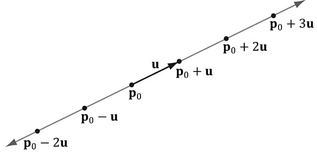
Figure C.1. A line described by a point p0 on the line and a vector u that aims parallel to the line. We can generate points on the line by plugging in any real number t.
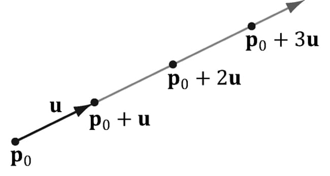
Figure C.2. A ray described by an origin p0 and direction u. We can generate points on the ray by plugging in scalars for t that are greater than or equal to zero.
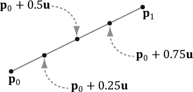
Figure C.3. We generate points on the line segment by plugging in different values for t in [0, 1]. For example, the midpoint of the line segment is given at t = 0.5. Also note that if t = 0, we get the endpoint p0 and if t = 1, we get the endpoint p1.
C.2 PARALLELOGRAMS
Let q be a point, and u and v be two vectors that are not scalar multiples of one another (i.e., u ≠ kv for any scalar k). Then the graph of the following function is a parallelogram (see Figure C.4):

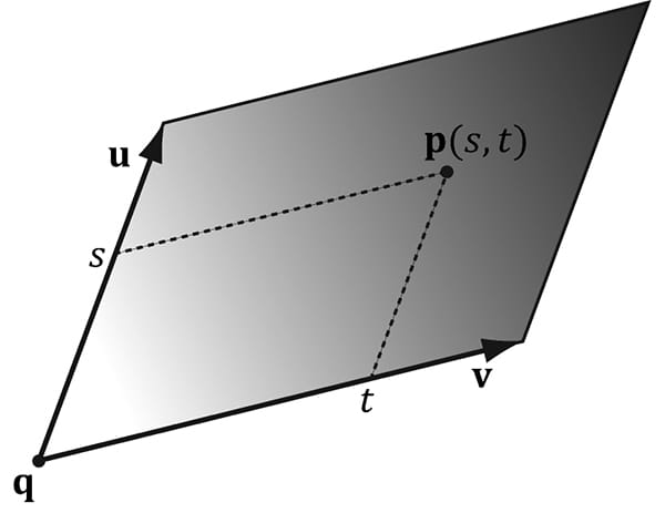
Figure C.4. Parallelogram. By plugging in different s, t ∈ [0, 1] we generate different points on the parallelogram.
The reason for the “u ≠ kv for any scalar k” requirement can be seen as follows: If u = kv then we could write:

which is just the equation of a line. In other words, we only have one degree of freedom. To get a 2D shape like a parallelogram, we need two degrees of freedom, so the vectors u and v must not be scalar multiples of each another.
C.3 TRIANGLES
The vector equation of a triangle is similar to that of the parallelogram equation, except that we restrict the domain of the parameters further:

Observe from Figure C.5 that if any of the conditions on s and t do not hold, then p(s, t) will be a point “outside” the triangle, but on the plane of the triangle.
We can obtain the above parametric equation of a triangle given three points defining a triangle. Consider a triangle defined by three vertices p0, p1, p2. Then for that s ≥ 0, t ≥ 0, s + t ≤ 1 a point on the triangle can be given by:

We can take this further and distribute the scalars:

where we have let r = (1 − s − t). The coordinates (r, s, t) are called barycentric coordinates. Note that r + s + t = 1 and the barycentric combination p(r, s, t) = rp0 + sp1 + tp2 expresses the point p as a weighted average of the vertices of the triangle. There are interesting properties of barycentric coordinates, but we do not need them for this book; the reader may wish to further research barycentric coordinates.
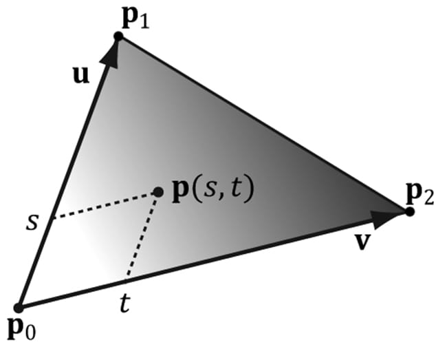
Figure C.5. Triangle. By plugging in different s, t such that s ≥ 0, t ≥ 0, s + t ≤ 1, we generate different points on the triangle.
C.4 PLANES
A plane can be viewed as an infinitely thin, infinitely wide, and infinitely long sheet of paper. A plane can be specified with a vector ν and a point p0 on the plane. The vector n, not necessarily unit length, is called the plane’snormal vector and is perpendicular to the plane; see Figure C.6. A plane divides space into a positive half-space and a negative half-space. The positive half space is the space in front of the plane, where the front of the plane is the side the normal vector emanates from. The negative half space is the space behind the plane.
By Figure C.6, we see that the graph of a plane is all the points p that satisfy the plane equation:

When describing a particular plane, the normal n and a known point p0 on the plane are fixed, so it is typical to rewrite the plane equation as:

where d = −n · p0. If n = (a, b, c) and p = (x, y, z), then the plane equation can be written as:
![]()
If the plane’s normal vector n is of unit length, then d = −n · p0 gives the shortest signed distance from the origin to the plane (see Figure C.7).
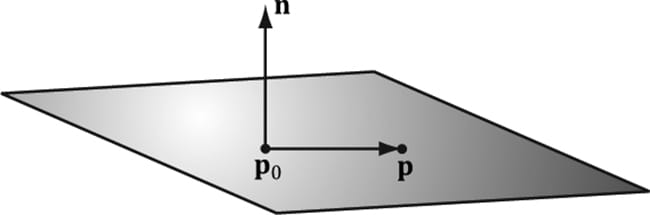
Figure C.6. A plane defined by a normal vector n and a point p0 on the plane. If p0 is a point on the plane, then the point p is also on the plane if and only if the vector p − p0 is orthogonal to the plane’s normal vector.]
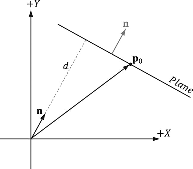
Figure C.7. Shortest distance from a plane to the origin.
|
|
To make the pictures easier to draw, we sometimes draw our figures in 2D and use a line to represent a plane. A line, with a perpendicular normal, can be thought of as a 2D plane since the line divides the 2D space into a positive half space and negative half space. |

C.4.1 DirectX Math Planes
When representing a plane in code, it suffices to store only the normal vector n and the constant d. It is useful to think of this as a 4D vector, which we denote as (n, d) = (a, b, c, d). Therefore, because the XMVECTOR type stores a 4-tuple of floating-point values, the DirectX Math library overloads the XMVECTOR type to also represent planes.
C.4.2 Point/Plane Spatial Relation
Given any point p, observe from Figure C.6 and Figure C.8 that
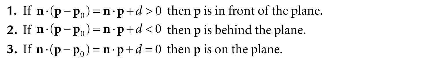
These tests are useful for testing the spatial location of points relative to a plane.
This next DirectX Math function evaluates n · p = d for a particular plane and point:
XMVECTOR XMPlaneDotCoord(// Returns n · p = d replicated in each coordinate
XMVECTOR P, // plane
XMVECTOR V); // point with w = 1
// Test the locality of a point relative to a plane.
XMVECTOR p = XMVectorSet(0.0f, 1.0f, 0.0f, 0.0f);
XMVECTOR v = XMVectorSet(3.0f, 5.0f, 2.0f);
float x = XMVectorGetX( XMPlaneDotCoord(p, v) );
if( x approximately equals 0.0f ) // v is coplanar to the plane.
if( x > 0 ) // v is in positive half-space.
if( x < 0 ) // v is in negative half-space.
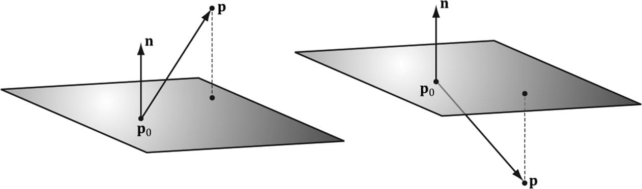
Figure C.8. Point/plane spatial relation.
|
|
We say approximately equals due to floating point imprecision. |
A similar function is:
XMVECTOR XMPlaneDotNormal(XMVECTOR Plane, XMVECTOR Vec);
This returns the dot product of the plane normal vector and the given 3D vector.
C.4.3 Construction
Besides directly specifying the plane coefficients (n, d) = (a, b, c, d), we can calculate these coefficients in two other ways. Given the normal n and a known point on the plane p0 we can solve for the d component:

The DirectX Math library provides the following function to construct a plane from a point and normal in this way:
XMVECTOR XMPlaneFromPointNormal(
XMVECTOR Point,
XMVECTOR Normal);
The second way we can construct a plane is by specifying three distinct points on the plane.
Given the points p0, p1, p2, we can form two vectors on the plane:

From that we can compute the normal of the plane by taking the cross product of the two vectors on the plane. (Remember the left hand thumb rule.)
![]()
Then, we compute d = −n · p0.
The DirectX Math library provides the following function to compute a plane given three points on the plane:
XMVECTOR XMPlaneFromPoints(
XMVECTOR Point1,
XMVECTOR Point2,
XMVECTOR Point3);
C.4.4 Normalizing a Plane
Sometimes we might have a plane and would like to normalize the normal vector. At first thought, it would seem that we could just normalize the normal vector as we would any other vector. But recall that the d component also depends on the normal vector: d = −n · p0. Therefore, if we normalize the normal vector, we must also recalculate d. This is done as follows:

Thus, we have the following formula to normalize the normal vector of the plane (n, d):

We can use the following DirectX Math function to normalize a plane’s normal vector:
XMVECTOR XMPlaneNormalize(XMVECTOR P);
C.4.5 Transforming a Plane
[Lengyel02] shows that we can transform a plane (n, d) by treating it as a 4D vector and multiplying it by the inverse-transpose of the desired transformation matrix. Note that the plane’s normal vector must be normalized first. We use the following DirectX Math function to do this:
XMVECTOR XMPlaneTransform(XMVECTOR P, XMMATRIX M);
Sample Code:
XMMATRIX T(…); // Initialize T to a desired transformation.
XMMATRIX invT = XMMatrixInverse(XMMatrixDeterminant(T), T);
XMMATRIX invTransposeT = XMMatrixTranspose(invT);
XMVECTOR p = (…); // Initialize Plane.
p = XMPlaneNormalize(p); // make sure normal is normalized.
XMVECTOR transformedPlane = XMPlaneTransform(p, &invTransposeT);
C.4.6 Nearest Point on a Plane to a Given Point
Suppose we have a point p in space and we would like to find the point q on the plane (n, d) that is closest to p. From Figure C.9, we see that

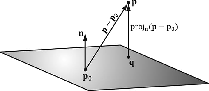
Figure C.9. The nearest point on a plane to a point p. The point p0 is a point on the plane.
Assuming ||n|| = 1 so that 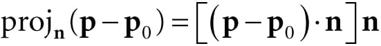
we can rewrite this as:

C.4.7 Ray/Plane Intersection
Given a ray p(t) = p0 + tu and the equation of a plane n · p + d = 0, we would like to know if the ray intersects the plane and also the point of intersection. To do this, we plug the ray into the plane equation and solve for the parameter t that satisfies the plane equation, thereby giving us the parameter that yields the intersection point:
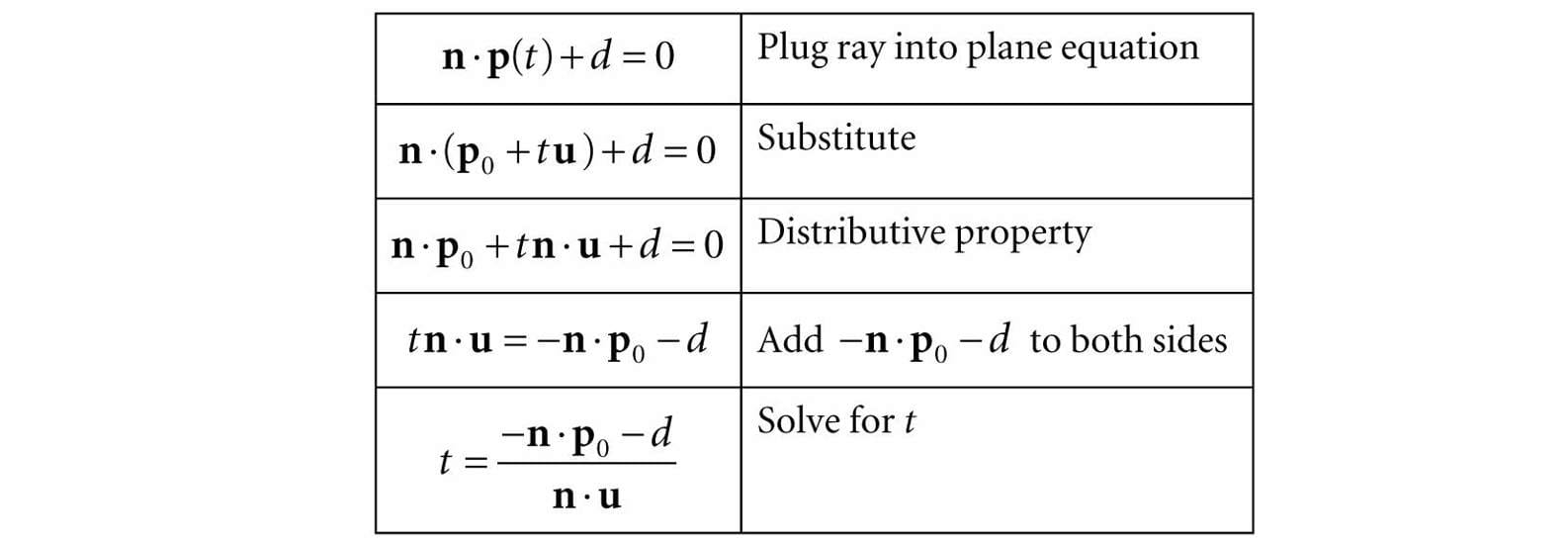
If n·u = 0 then the ray is parallel to the plane and there are either no solutions or infinite many solutions (infinite if the ray coincides with the plane). If t is not in the interval [0, ∞), the ray does not intersect the plane, but the line coincident with the ray does. If t is in the interval [0, ∞), then the ray does intersect the plane and the intersection point is found by evaluating the ray equation at 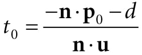
.
The ray/plane intersection test can be modified to a segment/plane test. Given two points defining a line segment p and q, then we form the ray r(t) = p + t(q − p). We use this ray for the intersection test. If t ∈[0, 1], then the segment intersects the plane, otherwise it does not. The DirectX Math library provides the following function:
XMVECTOR XMPlaneIntersectLine(
XMVECTOR P,
XMVECTOR LinePoint1,
XMVECTOR LinePoint2);
C.4.8 Reflecting Vectors
Given a vector I we wish to reflect it about a plane with normal n. Because vectors do not have positions, only the plane normal is involved when reflecting a vector. Figure C.10 shows the geometric situation, from which we conclude the reflection vector is given by:

C.4.9 Reflecting Points
Points reflect differently from vectors since points have position. Figure C.11 shows that the reflected point q is given by:

C.4.10 Reflection Matrix
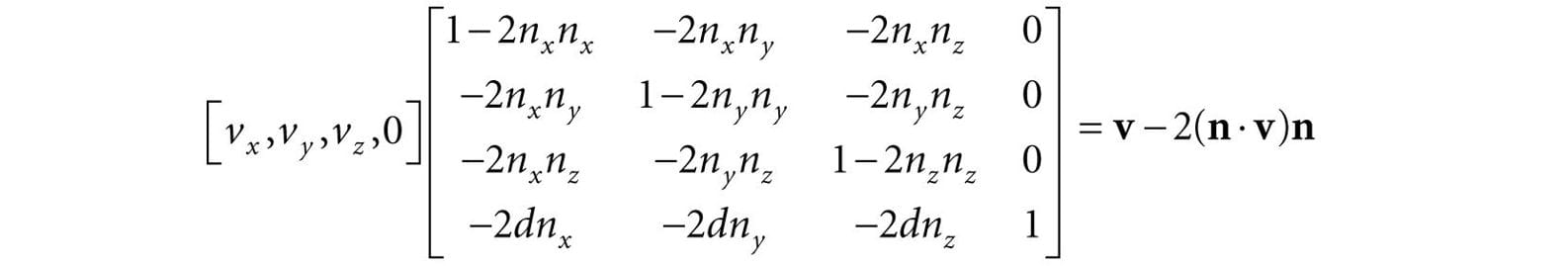
Let (n, d) = (nx, ny, nz, d) be the coefficients of a plane, where d = − n · p0. Then, using homogeneous coordinates, we can reflect both points and vectors about this plane using a single 4 × 4 reflection matrix:
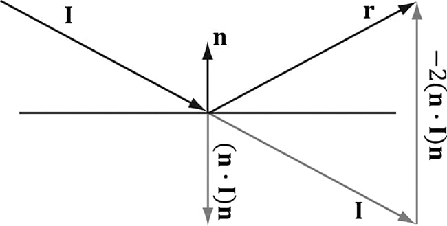
Figure C.10. Geometry of vector reflection.
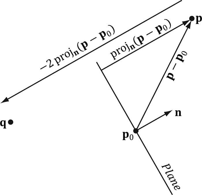
Figure C.11. Geometry of point reflection.

This matrix assumes the plane is normalized so that

If we multiply a point by this matrix, we get the point reflection formula:
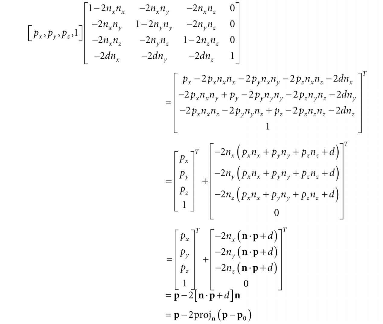
|
|
We take the transpose to turn row vectors into column vectors. This is just to make the presentation neater—otherwise, we would get very long row vectors. |
And similarly, if we multiply a vector by this matrix, we get the vector reflection formula:
The following DirectX Math function can be used to construct the above reflection matrix given a plane:
XMMATRIX XMMatrixReflect(XMVECTOR ReflectionPlane);
C.5 EXERCISES
1. Let p(t) = (1, 1) + t(2, 1) be a ray relative to some coordinate system. Plot the points on the ray at t = 0.0, 0.5, 1.0, 2.0, and 5.0.
2. Let p0 and p1 define the endpoints of a line segment. Show that the equation for a line segment can also be written as p(t) = (1 − t)p0 + tp1 for t ∈ [0, 1].
3. For each part, find the vector line equation of the line passing through the two points.
1. p1 = (2, −1), p2 = (4, 1)
2. p1 = (4, −2, 1), p2 = (2, 3, 2)
4. Let L(t) = p + tu define a line in 3-space. Let q be any point in 3-space. Prove that the distance from q to the line can be written as:

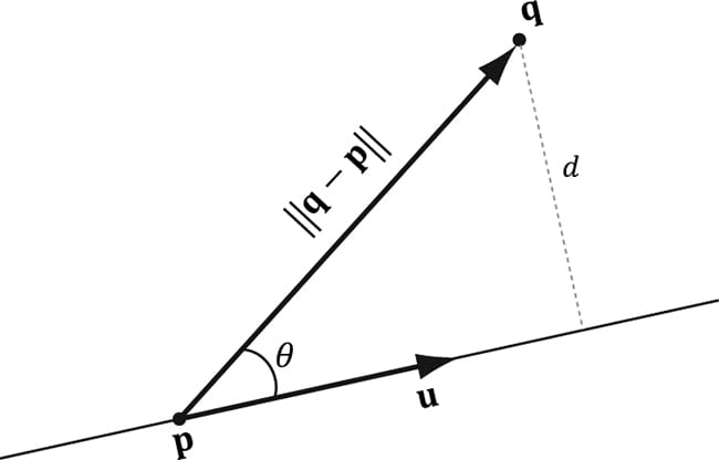
Figure C.12. Distance from q to the line.
5. Let L(t) = (4, 2, 2) + t(1, 1, 1) be a line. Find the distance from the following points to the line:
1. q = (0, 0, 0)
2. q = (4, 2, 0)
3. q = (0, 2, 2)
6. Let p0 = (0, 1, 0), p1 = (-1, 3, 6), and p2 = (8, 5, 3) be three points. Find the plane these points define.
7. Let 
be a plane. Define the locality of the following points relative to the plane: 
.
8. Let 
be a plane. Find the point on the plane nearest to the point (0, 1, 0).
9. Let 
be a plane. Find the reflection of the point (0, 1, 0) about the plane.
10.Let 
be a plane, and let r(t) = (−1, 1, −1) + t(1, 0, 0) be a ray. Find the point at which the ray intersects the plane. Then write a short program using the XMPlaneIntersectLine function to verify your answer.
All materials on the site are licensed Creative Commons Attribution-Sharealike 3.0 Unported CC BY-SA 3.0 & GNU Free Documentation License (GFDL)
If you are the copyright holder of any material contained on our site and intend to remove it, please contact our site administrator for approval.
© 2016-2026 All site design rights belong to S.Y.A.