Mastering Lambdas: Java Programming in a Multicore World (2015)

CHAPTER 6. Stream Performance

This book has put forward two reasons for using lambdas and streams: to get better programs, and to get better performance. By now, the code examples should have demonstrated the claim for better programs, but we have not yet examined the claims about performance. In this chapter, those claims will be investigated through the technique of microbenchmarking.

This is a dangerous business: results from microbenchmarking run the risk of being used to guide program design in unsuitable situations. Since the overwhelming majority of situations are unsuitable, that is a serious problem! For example, a programmer’s intuition is a highly unreliable guide for locating performance bottlenecks in a complex system; the only sure way to find them is to measure program behavior. So initial development, in which there is no working system to measure, is a prime instance of an unsuitable time for applying optimizations.

This is important, because mistakenly optimizing code that is not performance-critical is actually harmful.

• It wastes valuable effort, since even successful optimization will not improve overall system performance.

• It diverts attention from the important objectives of program design—to produce code that is well structured, readable, and maintainable.

• Source-code optimizations may well prevent just-in-time compilers from applying their own (current and future) optimizations, because these optimizations are tuned to work on common idioms.

That said, programmers enjoy learning about code performance, and there are real benefits to doing so. Foremost among these is the ability provided to developers by the Stream API to tune code—by choosing between sequential and parallel execution—without altering its design or behavior. This kind of unobtrusive performance management is new to the Java core libraries, but may become as successful and widespread here as it already is in enterprise programming. To take advantage of it, you need a mental model of the influences on the performance of streams.

However, even if you never act on that model directly, it can help to guide (but not dictate!) your design, complementing the mental model that programmers already have for the execution of traditional Java code.¹ In addition, the situations do exist in which optimization really is justified. Suppose, for a simple example, that you have identified a performance-critical bulk processing step and you now want to decide between the options for implementing it. Should you use a loop or a stream? If you use a stream, you often have a choice of different combinations of intermediate operations and collectors; which will perform best? This chapter will present results like Figure 6-1 to help answer such questions:

Figure 6-1 might be an interesting and useful result, but we need to know more. As it stands, it provides no information about the experimental conditions under which its result was obtained. The results will have been influenced both by factors external to the benchmark—varying system load, the behavior of other processes, network and disk activity, the hardware, operating system, and JVM configurations—and by properties of the benchmark itself: the data being processed and the operations that were performed.

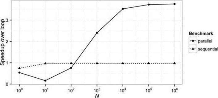
FIGURE 6-1. Stream performance: sequential and parallel streams

Obviously, this is a problem; we want to be able to discuss performance of stream operations without taking all these factors into consideration. How can we get meaningful results from highly simplified observations of such complex systems? To draw an analogy—only a little far-fetched—think of the difficulty of trialing a new drug on humans. The goal of a trial might be simple—to discover if a drug is effective in treating a certain disease—but achieving it isn’t simple at all: you can’t just administer the drug to a person with the disease and observe whether they are cured. Many factors can influence the result: the background health of the subject, their diet, age, gender, and often many others. All of these factors can affect the result for any individual.

Of course, working computer systems are not nearly so complex as biological systems, but they are complex enough for observational experiments to share the problem: just as you can’t draw a conclusion about a drug’s effectiveness by simply administering it to someone and observing the outcome, you can’t change a line of code in a working system and expect to get a useful result simply by observing the outcome. In both cases there are too many variables involved. In the next section we will look at an experimental method for eliminating these effects as far as we can. Then, in the rest of the chapter, we’ll apply that method to measuring performance of stream operations.

Many of the experiments in this chapter are derived from examples used earlier for explaining stream programming techniques. These examples almost all illustrate the use of reference streams; for this reason, and because in practice it is reference streams that will raise the important performance questions, it is these rather than primitive streams that are the main focus of this chapter.

6.1 Microbenchmarking

Our aim is to discover the execution cost of a particular code fragment. But the argument in this chapter so far has been that a measurement of that cost is meaningful only in a working system under realistic load. Profiling or metering a production system is often not practicable; the alternative, of simulating the production system on a load-testing platform, is more feasible but still involves the difficulty of setting up an environment that reproduces the production system in all aspects: hardware and operating system configuration, demand on resources by other processes, the network and disk environments, and of course simulated typical and extreme loads.

A more practicable alternative is microbenchmarking, which compares two different code fragments operating in an isolated (and unrealistic) system. Each of these results will be meaningless in absolute terms, but the comparison between them can be meaningful—provided all those aspects are controlled. The idea of a controlled experiment is simple in principle. If all the factors listed earlier (the hardware and software environments, the system load, and so on) are held constant and only the code being compared is allowed to vary, then variation in the results must be due to what has been changed.

6.1.1 Measuring a Dynamic Runtime

Even when we have succeeded in controlling external influences on program behavior, other pitfalls await. Suppose our experiment follows this common template:

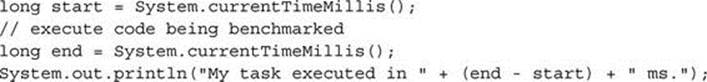
The apparent simplicity of this pattern hides some serious difficulties. Some of these relate to the measuring process itself, particularly for short run times: System.currentTimeMillis may be much less accurate than its name suggests, because it depends on a system clock that on some platforms may be updated only every 15ms or less. A better alternative on many platforms may be System.nanoTime, whose update resolution is typically only microseconds (but which can add significant measurement overhead). Further, these system calls measure elapsed time, so they include overheads like garbage collection.

The JVM itself also contributes misleading effects. Many of these relate to the dozens of optimizations that are applied by the bytecode-to-native compiler. Here are just three examples of the type of measurement problems that JVM operation can produce.

Warmup effects Measuring the cost of performing, say, the first 100 executions of a code fragment will often produce quite different results from taking the same measurement a minute later. A variety of initialization overheads may contribute to the earlier measurement, for example class loading—an expensive operation, which the JVM delays until the classes concerned are actually required. Another potent source of inaccuracies is provided by JIT compilation: initially the JVM interprets bytecode directly, but compiles it to native code when it has been executed enough times to qualify as a “hot spot” (and then continues to profile it in the interests of possible further optimization). The compilation overhead, followed by markedly improved performance, will give results far out of line with the steady-state observations that we require.

Dead code elimination A recurrent problem in writing microbenchmarks is ensuring that something is done with the result of the computation. Dead code elimination (DCE), an important compiler optimization, has the purpose of eliminating code that has no effect. For example, the following code is a naïve attempt to measure the cost of addition:

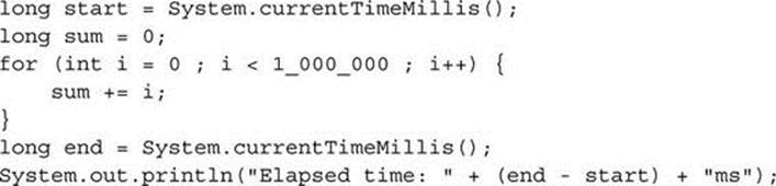
Running this test on a modern JVM will result in very low execution times, because the compiler can detect that since sum is never used, it is unnecessary to calculate it and therefore unnecessary to execute the loop at all. In this case, there is a simple remedy: including the final value of sumin the output statement should ensure that it has to be calculated, although even then a compiler may detect that it can use an algebraic formula to calculate it without iterating; in general it is quite difficult to devise ways of preventing the compiler from applying DCE without distorting the measurements by introducing expensive new operations.

Garbage collection This is not a result of optimizations, but is a problem inherent in measuring programs that use automatic memory management: almost all benchmarks create objects, and some of these will become garbage while the benchmark is running. Eventually the garbage collector will be called, and its execution will contribute to the timing results. It may be possible to reduce this effect by manually triggering garbage collection before a measurement, but this might be unrealistic: in fact, it may be desirable to include garbage collection effects in the benchmark measurements if they will have a significant impact on performance in production. A better possibility may be to run the programs long enough for these costs to be amortized over many iterations.

6.1.2 The Java Microbenchmarking Harness

These effects, and many others, must be controlled to ensure that we have measured what we wanted to. Controlling them is such a common—and difficult—problem that benchmarking frameworks have become popular. These frameworks create custom test classes specifically designed to avoid the numerous pitfalls of microbenchmarking. The test classes are synthesized by the framework from benchmarking source code that you supply. Examples of benchmarking frameworks are Google Caliper (http://code.google.com/p/caliper) and the framework used to obtain the results of this chapter, the Java Microbenchmarking Harness (JMH) (http://openjdk.java.net/projects/code-tools/jmh).

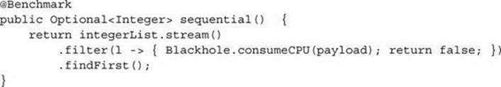
JMH helps to solve the problems listed in the previous section. For example, the JMH API includes a static method, Blackhole.consumeCPU, which consumes CPU time in proportion to its argument without side-effect and without risking DCE and other optimizations. (The absolute amount of time used is unimportant, because consumeCPU will only ever be used for comparisons between microbenchmarks.)

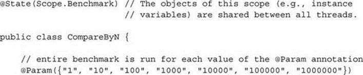
To create a benchmark using JMH, you only have to annotate a method with @Benchmark. JMH has different modes of use; in the throughput mode, it executes each annotated method repeatedly for a time period you specify, automatically passing the returned value to the methodBlackhole.consume to avoid DCE. For example, here is one of the three methods used to generate the graph at the beginning of this chapter. In this case the returned value will always be an empty Optional, but the requirement to return it means that the VM must evaluate the filter predicate for every stream element:

6.1.3 Experimental Method

Finally, we apply two of the standard safeguards of experimental science to the results of our experiments.

Statistics Given the number of factors that we now know affect microbenchmarking measurements, we can hardly expect that the same experiment, repeated several times, will produce exactly the same result; the influence of different external factors will vary from one set of observations to another. We can calculate a point estimate (such as the mean) for the most probable value, but that will have little meaning if external factors dominate the experiments. If we can assume that the effects of external factors are varying randomly, then running the same experiment a number of times can increase our confidence in the result. This can be quantified in a confidence interval (CI)—a range of values within which we can state with a degree of certainty (conventionally 95%) that the “true” value lies—that is, the value that we might get from many experiments. The larger the experiment, the narrower the confidence intervals that we can obtain.

Confidence intervals give us a useful indicator of experimental significance: if CIs from two different situations do not overlap, it is an indication that these situations really do give different results, always assuming that the other factors are varying randomly in a way that would not bias one set compared to another. In practice, for the experiments of this chapter, the variation between conditions is small compared to the differences in the means, and the number of trials is large enough that the confidence intervals are in practice too small to appear on the plots.

Open peer review Like all scientific experiments, performance measurements are subject to flaws and bias. A partial safeguard against these sources of error is to enable open peer review of measurement experiments. This means publishing not only the summarized results, but also enough detail about the experimental conditions to enable others to reproduce and check them. This information includes the hardware, operating system, and JVM environments, as well as statistical information about the results. What follows is an example: a benchmark and its resulting data as used for Figure 6-1. Instead of tediously reproducing this information for each experiment in this chapter, a URL refers to the location on the book website of the full setup; as the experiments are easy to reproduce, raw experimental results are not usually provided.

JMH was used to run these benchmarks with their default settings—for each value of limit, it starts a new JVM, then performs the following sequence (called an “iteration”) for each of the annotated methods:

1. For the warmup, it executes the method repeatedly for one second, 20 times over.

2. For the measurement, it again executes the method repeatedly for one second, 20 times over; this time, it records the number of times the method could be called in each one-second run (the “Score”).

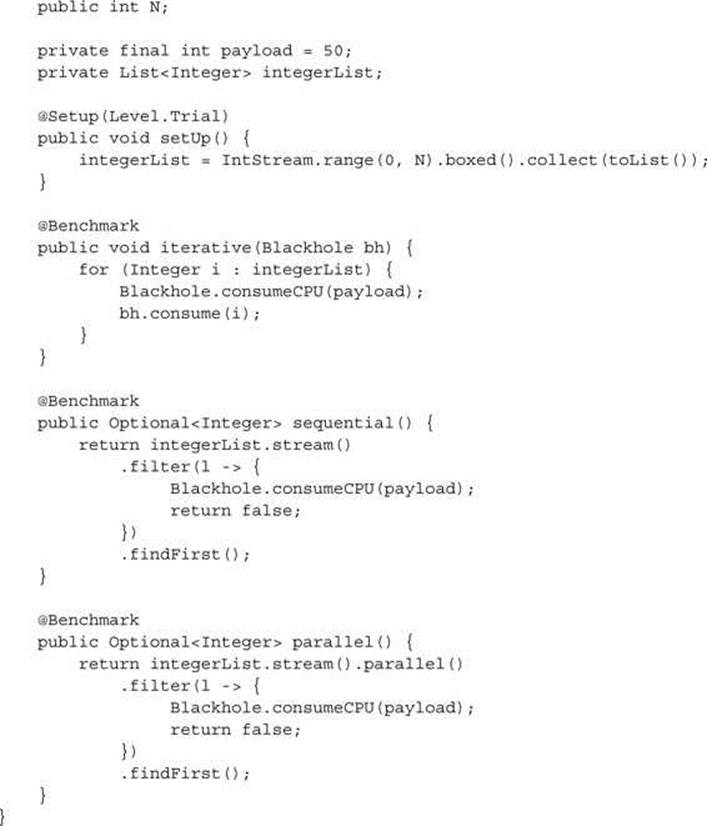
Each line in Table 6-1 shows, for a given data set size, the mean execution count and the confidence interval for a sample of 20 iterations.

TABLE 6-1. Sample Results for the Benchmark of Figure 6-3

This table shows the results, somewhat simplified, of executing the benchmark above on JDK1.8u5, running Linux (kernel version 3.11.0) on an Intel Core 2 Q8400 Quad CPU (2.66 GHz) with 2MB L2 cache. The column headed “Error (99.9%)” shows the spread of values in the 99.9 percent confidence interval (99.9% is the JMH default CI, very demanding by normal statistical standards).

The rest of this chapter will present microbenchmarking results in the form of graphs like Figure 6-1 without providing this level of detail. But it is important that you know everything should be available: the full conditions for each experiment, the statistical methods used to prepare the presentation, and, where necessary, the raw results. This should give you confidence that you can review the method of the experiment, if necessary repeat it for yourself, and—most importantly—design and execute your own measurement experiments.

You should read what follows with a warning in mind: developments in hardware and in the Java platform will sooner or later change many of the trade-offs discussed here, generally in favor of parallelism. Like all discussions of specific aspects of performance, this material comes with a use-before notice. Only the actual date is missing!

6.2 Choosing Execution Mode

This book has presented the opportunity of parallelism as a major motivation for programming with streams. But until now there has been no discussion of when you should actually take that opportunity.² There are three sets of factors to consider.

Execution context What is the context in which your program is executing? Remember that the implementation of parallel streams is via the common fork/join pool, which by default decides its thread count on the basis of a query to the operating system for the number of hardware cores. Operating systems vary in their responses to this query; for example, they may take account of hyperthreading, a technology that allows two threads to share a single core, so that the core does not have to idle when one thread is waiting for data. In a processor-bound application, that may very well result in parallelizing over more threads than can be used at one time.

Another aspect of the execution context is competition from other applications running on the same hardware. An implicit assumption in the common fork/join pool configuration is that there are no other demands on the hardware while parallel operations are being performed. If the machine is already heavily loaded, then either some of the fork/join pool threads will be starved of CPU time, or the performance of the other applications will be degraded.

If either of these problems means that you want to reduce the number of threads in the common fork/join pool—or indeed, if you want to change it for any other reason—the system property java.util.concurrent.ForkJoinPool.common.parallelism can be set to override the default configuration of the fork/join pool. Of course, if you do set this property, you then have the challenging task of justifying your change by measuring the resulting change in your application’s performance!

In addition to external competition, you should consider internal competition in deciding whether to execute streams in parallel. Some applications are already highly concurrent; for example, consider a web server, which will perform best if it can assign each user request to a single core for execution. That strategy is obviously incompatible with one that attempts to take over all cores for the execution of a single request.

Workload As we saw in §5.2, a lot of machinery is required to set up parallel streams. The delay introduced by this setup needs to be balanced by the time saved subsequently by the simultaneous processing of the stream elements. Without parallelism, the elapsed execution time of a series of N tasks, each requiring Q time individually, is N × Q. With perfect parallelization over P independent processors, it is N × Q %P . The difference between these two amounts must outweigh the overheads of parallelization. Clearly, the larger that N and Q are, the more likely that is to be the case. Figure 6-3 shows the relative speedup over a loop of sequential and parallel stream execution for a pure processing task of three different durations. The operation cost Q is provided by the JMH method Blackhole.consumeCPU. Its value varies from one machine to another; this experiment was performed on the Q8400 mentioned earlier, on which Q was measured (to give a rough idea of its value) at about five nanoseconds. Figure 6-3 shows break-even points (the crossing point of the lines) between parallel and sequential execution at values of N × Q of ∼40 microseconds, around five times less than the range informally reported by the Oracle team. Figure 6-2 shows a similar N × Q response for the first stream program developed in this book, the “maxDistance” problem from §1.2.

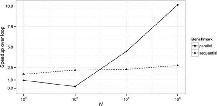
FIGURE 6-2. “maxDistance” program performance (http://git.io/r6BtKQ)

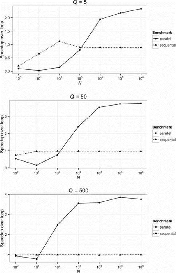
FIGURE 6-3. Stream performance: N*Q model (http://git.io/4NIuqw)

The optimal value of P for parallel execution is not an absolute, but depends on the workload. If N × Q is insufficiently great, then the overhead of partitioning the workload will dominate the savings made by parallelization. The larger the workload, the greater will be the speedup produced by an increased processor count.³

Spliterator and collector performance These are discussed in more detail in §6.7 and §6.8. For now, it is enough to notice that splitting by sources and concurrent accumulation by collectors becomes increasingly important as Q decreases; a high Q value tends to make intermediate operations into the pipeline bottleneck, making parallelism more worthwhile. In the situation where Q is low, by contrast, concurrent performance of the stream source and terminal operation become more important in deciding whether to go parallel.

One problem of applying this model lies in the difficulty of estimating Q in real-life situations, and in the fact that stream operations with high Q are unlikely to be as simple as in this experiment, as we saw in the larger examples of Chapters 4 and 5. If in fact they are, then measuring the cost of intermediate pipeline operations is straightforward and the results of this experiment will be directly useful to you; but, in practice, more complex intermediate operations will usually involve some I/O or synchronization, resulting in fewer gains from going parallel. As always, if you are in doubt, be prepared to repeat this experiment, adapting it to your own requirements.

6.3 Stream Characteristics

The preceding section represented the question of whether to go parallel very simply. This was made possible by ignoring the differences between the behavior of different streams and of different intermediate operations. In this section we will look more closely at the properties of streams, and in later sections we will see how different operations can make use of these to choose good implementation strategies—or, in some cases, be restricted by them to suboptimal strategies. For example, maintaining element ordering during parallel processing incurs a significant overhead for some intermediate and terminal operations, so if a stream’s elements are known to be unordered—for example, if they are sourced from a HashSet—then stream operations can make performance gains by not preserving element ordering.

Streams expose metadata like this through characteristics, which can be either true or false; in this case, an operation would check whether the characteristic ORDERED was true for this stream. The characteristics of a stream S are initially defined by its source (in fact, stream characteristics are defined as fields of the Spliterator interface); subsequently, a new stream produced by an intermediate operation on S may, depending on the operation, have the same characteristics as S, or may have some removed or new ones added. Here, for example, is a selection of the characteristics of each stage in a pipeline.

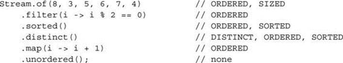
We will consider ORDERED in the next section; here is the meaning of the others:

• SORTED: Elements of streams with this characteristic are sorted in their natural ordering—that is, their type implements Comparable, and they have been sorted using its compareTo method. Stream elements may have been sorted in other orders if a Comparator has been defined and used for the purpose, but such streams do not have the SORTED characteristic. So, for example, a stream whose source is a NavigableSet has the characteristic SORTED, but only if the implementation was created using a default constructor rather than one that accepts a Comparator. By contrast, this characteristic will not be set in a stream sourced from a List.

An example of the use of this characteristic is in sorting: the operation of sorting in natural order can be optimized away entirely when applied to a stream with the characteristic SORTED. For another example, distinct on a sequential sorted stream can apply a simple algorithm to avoid storing elements: an element is added to the output stream only if it is unequal to its predecessor.

• SIZED: A stream has this characteristic if the number of elements is fixed and accurately known. This is true, for example, of all streams sourced from non-concurrent collections. These must not be modified in any way during stream processing, so their size remains known. Concurrent collections, by contrast, may have elements inserted or deleted during stream processing, so the number of elements cannot be accurately predicted before the stream is exhausted. Streams from most of the non-collection stream sources in §5.1 are not sized.

An example of an optimization that makes use of SIZED is accumulating to a collection; this is more efficient if dynamic resizing of the collection can be avoided by creating it with the appropriate size.

• DISTINCT: A stream with this characteristic will have no two elements x and y for which x.equals(y). A stream sourced from a Set will have this characteristic, but not one sourced from a List.

For an example of its usefulness, the operation distinct can be optimized away entirely when applied to a stream with this characteristic.

6.4 Ordering

Of the characteristics listed in the previous section, ordering is the one that most deserves attention in a performance chapter, because dispensing with ordering can remove a big overhead from parallel stream processing for some pipelines. Moreover, as Chapter 1 emphasized, this is the characteristic that we are most likely to impose unnecessarily from our long familiarity with iterative processing—think of the friend in §1.1.1 who insisted that you put the letters for mailing into the letterbox in alphabetical order. So it is very much worthwhile distinguishing those cases in which ordering really does matter.

A stream is said to have an encounter order if the ordering of the elements is semantically significant. For example, take List: given a sequence of operations to add elements to a List, its contract specifies how those elements will be positioned and guarantees to preserve their ordering when returning them, for example by iteration. Now consider processing the elements of a List using a stream:

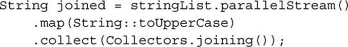
You would be surprised and disappointed if the string joined did not reflect the ordering of stringList. You can think of encounter order as the property by which a stream preserves the “position” of elements passing through it. In this case because List has an encounter order (data structures can also have this property), so too does the stream, and the spatial arrangement of the elements is preserved into the terminal operation. For example, if stringList has the value ["a", "B", "c"], then joined is guaranteed to be "ABC", not "BAC" or "CAB".

By contrast, if the stream source has no encounter order—if it is a HashSet, say—then there is no spatial order to be preserved: the stream source has no encounter order and neither has the stream.⁴ Since the stream has been explicitly identified as parallel, we must assume that the chunks of the collection may be processed by different threads on different processors. There is no guarantee that the results of processing, used by the joining method as soon they are available, will arrive in the order in which processing began. If your subsequent use of the concatenated string doesn’t require ordering—say, for example, that you will use it only to extract the occurrence count of each character—then to specify it may hurt performance and will be confusingly at odds with the purpose of the program.

You should not need to understand detail of the stream class implementations to apply this general rule. For example, you might not expect that unordering a stream would improve performance in a program like this:

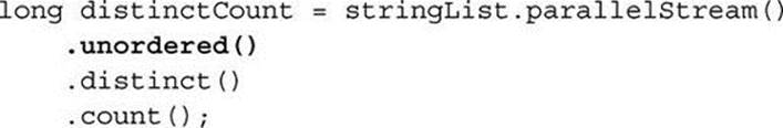
but in fact performance on large data sets improves by a factor of 50 percent (http://git.io/i6frOw). The reason is that distinct is implemented by testing membership of the set of previously seen elements, and if the stream is unordered a concurrent map can be used. But this is an implementation detail that might well change in the future: the principle—that you should be aware of ordering and use it only when necessary—will not change.

Originally the term “encounter order” was defined in contrast to “temporal order,” used to describe the situation in which the elements of a stream are ordered according to the time at which they are produced. Now that situation is described as “unordered”: a shorthand way of expressing the idea not that a stream has no order, but rather that you cannot rely on the order that it has. It is easy to show that there is no necessary relationship between temporal and encounter order for parallel streams, for example by observing the effect of mutating a threadsafe object from within a pipeline operation. Executed sequentially, this code

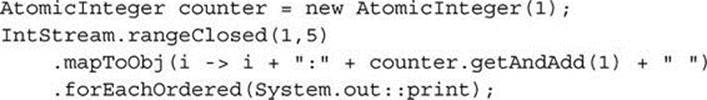
usually produces the output

1:1 2:2 3:3 4:4 5:5

whereas when executed in parallel, you can never predict the ordering of side-effects:

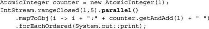
produces (for example)

1:2 2:1 3:5 4:4 5:3

But notice that in neither case can you depend on the order of side-effects.

6.5 Stateful and Stateless Operations

Intuitively, it is clear that some intermediate operations lend themselves more easily to parallelization than others. For example, the application of map to a stream can obviously be implemented by an element-by-element evaluation of map’s behavioral parameter applied to the stream elements. By contrast, sorted, the operation of sorting the elements of a stream, cannot complete until it has accumulated all the values that the stream will yield before exhaustion. Because map can process each stream element without reference to any other, it is said to be stateless. Other stateless stream operations include filter, flatMap, and the variants of map and flatMap that produce primitive streams. Pipelines containing exclusively stateless operations can be processed in a single pass, whether sequential or parallel, with little or no data buffering.

Operations like sorted, which do need to retain information about already-processed values, are called stateful. Stateful operations store some, or even—if multiple passes are required—all, of the stream data in memory. Other stateful operations include distinct and the stream truncation operations skip and limit. The library implementations use various strategies to avoid in-memory buffering where possible; these make it very difficult to predict how a stateful operation will influence parallel speedup. For example, a naïve benchmark measuring the performance of sortedon a stream of Integer can report parallel speedup of 2.5 on four cores (http://git.io/6kdkDw) where the conditions happen to be right for optimization. On the other hand, the Oracle team experienced frustration with the unexpected and unintuitive difficulty of efficiently parallelizing limit, which remains an operation to use with caution in a parallel stream. Fortunately, further work on the stream library, implementing further optimizations and changing existing ones, will continually improve the situation for library users.

6.6 Boxing and Unboxing

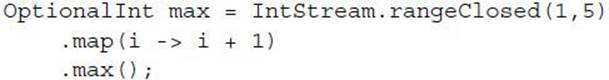
An important motivation for the introduction of primitive streams was to avoid boxing and unboxing overheads. In §3.1.2, we considered a simple task to manipulate number streams. One program used a primitive stream:

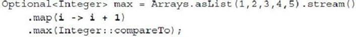
and the other a stream of wrapper values:

The performance of these two programs is compared for different stream lengths in Figure 6-4, which includes, for reference, a similar comparison for iterative programs. As expected, the code without boxing easily outperforms the boxed code; for large data sets the speedup approaches an order of magnitude.

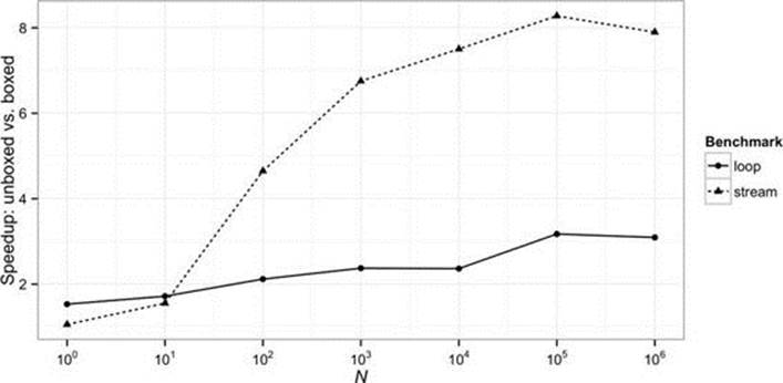
FIGURE 6-4. Unboxed vs. boxed performance (http://git.io/YB9V6g)

6.7 Spliterator Performance

The influence of the stream source on sequential stream performance is relatively straightforward: if the source can provide values quickly enough to keep the stream processes supplied with data, it will have little influence on performance. If not, it will form the bottleneck on the overall process. For parallel streams, the question is more complex, since two complementary processes—splitting and iteration—are needed to decompose the source data to supply parallel threads. A data source may provide a fast implementation of one but be unable to support the other efficiently. For example, IntStream.iterate may be able to deliver values extremely quickly if its UnaryOperator is efficient, but since each value cannot be calculated until its predecessor is known, it provides little opportunity for splitting, so parallel streams using it as a source may show no speedup over sequential execution. Among common stream sources, the most efficiently splittable are arrays, ArrayList, HashMap, and ConcurrentHashMap. The worst are LinkedList, BlockingQueue implementations, and I/O-based sources.

Stream-bearing I/O methods and others like iterate can sometimes benefit from parallelization, however, if an extra processing step is inserted, pre-buffering their output in an in-memory data structure, as the discussion of BufferedReader (p. 115) suggested. Generalizing, this leads to the conclusion that programs using the Stream API will gain most from parallel speedup when their data source is an in-memory, random-access structure lending itself to efficient splitting. (Of course, that does not prevent programs with other data sources benefiting from the Stream API in other ways.)

A realistically sized example that illustrates this is the program of Chapter 5 simulating grep -b. Reading a sequentially accessed file into a MappedByteBuffer brings the data into a highly suitable form for parallelization. An experiment to measure the performance of this program (http://git.io/-CziKQ) compares the speed of splitting a MappedByteBuffer into lines by three different algorithms: iterative, stream sequential, and stream parallel. The overhead of setting up the MappedByteBuffer is excluded from the measurements in order to focus on the efficiency of the splitting algorithm. The results are relatively independent of the data set size: sequential stream processing is between 1.9 and 2.0 times as fast as iterative processing for files of between 10,000 and a million lines; over the same range, parallel processing is between 5.2 and 5.4 times as fast as iterative processing. This is unsurprising, given the efficient splitting algorithm developed in §5.4.

6.8 Collector Performance

The behavior of terminal operations, like that of stream sources, is more complex for parallel than for sequential streams. In the sequential case, collection consists only of calling the collector’s accumulator function, which, if it consumes values from the stream quickly enough, can avoid being a bottleneck for the entire process. For parallel streams, the framework treats collectors differently according to whether they declare themselves CONCURRENT, by means of the characteristics by which collectors report their properties. A concurrent collector guarantees that its accumulator operation is threadsafe, so that the framework does not need to take responsibility for avoiding concurrent accumulator calls as it must do for non-threadsafe structures. In principle, avoiding the framework overhead of managing thread confinement should lead to better parallel performance. This can be realized in practice, as we shall see, by choosing appropriate data sets and configuration parameters.

Collectors report only two other characteristics besides CONCURRENT: a collector can have IDENTITY_FINISH, which tells the framework that it need not make provision for a finisher function, and UNORDERED, which tells the framework that there is no need to maintain an encounter order on the stream, as the collector will discard it anyway.

6.8.1 Concurrent Map Merge

The concurrent collectors provided by the library are obtained from the various overloads of the Collector methods toConcurrentMap and groupingByConcurrent. Those that use a framework-supplied ConcurrentMap implementation (rather than allowing you to provide a ConcurrentMapsupplier) all rely on ConcurrentHashMap (CHM). The performance characteristics of these collectors need some explanation, which all potential users of these collectors should understand. A naïve benchmark (http://git.io/YXyvpg) shows worse performance for groupingByConcurrent than forgroupingBy for any data set. Profiling shows that groupingByConcurrent is slowed by frequent resizing of the CHM; creating the CHM with an initial size sufficient to avoid resizing improves performance by about 30 percent, even for a data set of only 1000 elements. If the comparison is made fair, however—that is, if the initial size of the HashMap used by groupingBy is also increased—it is still unfavorable to groupingByConcurrent, since resizing is a major overhead for HashMap as well.

But we are now in more familiar territory, in which a slower process—in this case, adding an element to CHM as against adding one to HashMap—is compensated for large data sets by the ability to perform the slower operation in parallel. With presizing chosen to achieve a load factor of 0.5 (http://git.io/HAiaQQ), the relative performance shows a pattern, by now familiar, of parallel speedup increasing with increased data size past 100,000 elements (Figure 6-5).

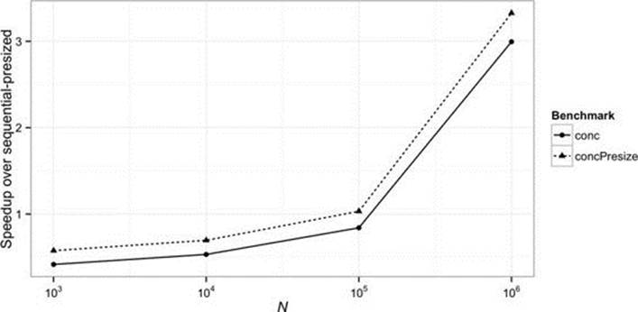
FIGURE 6-5. groupingByConcurrent vs. groupingBy

In fact, Figure 6-5 still does not tell the whole story. Sequential groupingBy creates new objects, so garbage collection becomes a factor in performance. Parallel GC biases the experiment in favor of sequential groupingBy because the cores unused by the sequential operation are available to run GC in parallel, hiding its cost. Running the same test with four measurement threads (supplying the option -t 4 to JMH) results in a break-even point below 10,000 elements.

6.8.2 Performance Analysis: Point Grouping

The “point grouping” collector of §4.3 is designed to be a good case for parallelization; although the data structure being created is a linked series of non-threadsafe ArrayDeques, all the collector operations on them are fast, with no iteration involved, so there is relatively little contention during the collection process. Run sequentially, the program of §4.3 (http://git.io/XdvZ3w) has a very similar performance profile to its iterative equivalent; the speedup of parallel over sequential execution is about 1.8 for a stream with no payload on a four-core machine, rising to 2.5 for a payload of 100 JMH tokens per element.

6.8.3 Performance Analysis: Finding My Books

The last collector program to be analyzed here is from §4.3.2: it is the program to find the displacement of each of my books along its shelf, given the page count of the preceding volumes. Following the analysis of concurrent map merging (§6.8.1), we should not be surprised to find that this collector, which is specified to produce a map, must be used with caution as the terminal operation for a parallel stream. Indeed, as it stands, the program (http://git.io/aMoy6w) is slower than the equivalent iterative version by about 40 percent. Several elements contribute to this, each of which might be mitigated in a real-life situation:

• This problem is an example of a prefix sum, in which the value of every element depends on the values of the preceding ones. In a naïve parallel algorithm for prefix sum, like this one, the total cost of the combine operations (that is, the total delay imposed by them) is proportional to the size of the input data set, regardless of the level of parallelism in use.⁵ The gravity of this problem depends on the cost of the combine operation; in this case, streaming the right-hand Deque into an intermediate List imposes an overhead that reduces speedup, for an intermediate workload, by about 20 percent compared to a simple iterative updating of the right-hand Deque before it is merged with the left-hand one.

• The finisher accumulates the results into a ConcurrentHashMap, whose initial size is currently left at the default value (16). For a realistically sized data set, this will result in numerous resizes, expensive for ConcurrentHashMap and one that generates a great deal of garbage—in fact, garbage collection costs dominate the unrefined program, so performance measurements do not give a useful indication of its performance in isolation. Presizing the CHM provides the biggest single contribution to improving performance. Even so, collecting to a Map is always an expensive operation; if the problem specified a linear data structure to hold the result, allowing the finisher simply to be omitted, parallel speedup over iterative processing would increase by about 40 percent for the same workload.

• The program as presented in Chapter 4 does no processing on the Book objects before they are collected. In this, it places parallel stream processing at a possibly unrealistic disadvantage—in real-life situations, preprocessing before collection will usually be required. As with all parallel stream programs, the greater the proportion of program workload that can be executed by intermediate operations using the fork/join pool, the greater the parallel speedup that can be achieved.

When these three changes are applied (http://git.io/wZe_tg), the parallel stream program shows a speedup of 2.5 (for four cores) over the sequential version, for a data set of a million elements, each requiring 200 JMH tokens to process.

6.9 Conclusion

The last example emphasizes again that the parallelization mechanism of the Stream API is by no means bound to produce performance improvement. To achieve that, your application must fall into the focus area for fork/join—CPU-bound processing of in-memory, random-access data—and must satisfy the other conditions discussed in this chapter, including the requirements for sufficiently high data set size and per-element processing cost. Fork/join parallelism is no silver bullet; the good news, however, is that your investment in writing parallel-ready code will not be wasted, whatever the outcome of your performance analysis. Your code will be better and, when advances in technology change the cost-benefit balance of going parallel, it will—as the name suggests—be ready.

____________

¹Unfortunately, the commonplace mental model for performance is itself sadly out of date; many programmers are unaware of JIT optimizations or the effect of hardware features like pipelining and multicore CPUs.

²Recall from §3.2.3 that all streams expose the methods parallel and sequential, which set the execution mode for an entire pipeline. That section makes the point that if there is more than one of these method calls on a single pipeline, it is the last one that decides the execution mode.

³This informal statement appeals to Gustafson’s law, which reframes the well-known analysis of Amdahl’s law to draw a less pessimistic conclusion. In contrast to Amdahl’s law, which sets very tight limits on the parallel speedup attainable with a fixed N and varying P, the scenario for Gustafson’s law is one in which N scales with P, giving a constant run time (seehttp://www.johngustafson.net/pubs/pub13/pub13.htm).

⁴Note that although you might expect all Set implementations to be intrinsically unordered, encounter order for a collection actually depends on whether the specification defines an iteration order: among the Collections Framework implementations of Set, that is the case for LinkedHashSet and for the implementations of the Set subinterfaces SortedSet and NavigableSet.

⁵Java 8 provided java.util.Arrays with various overloads of a new method parallelPrefix for computing prefix sums efficiently, but this innovation has not yet reached the Stream API.