Excel Bootcamp: Learn the Basics of Microsoft Excel (2016)

Chapter 3. Formulas and Functions

Formulas in Excel

When working on spreadsheets, you have to add, subtract, multiply, or divide values. That means each spreadsheet program must be able to accept, reference, and process numeric values. In Excel, however, mathematical formulas work on cells, not on the values themselves. This is because values, regardless of their type, are prone to changes. Formulas can be ruined if the values that they need will undergo unplanned alterations.

For example, you entered some numbers into B1 and B2. Since you are using Excel, you won’t type the numbers themselves in order to apply mathematical formulas. You just have to specify the cells that hold them and the mathematical operation that you want to apply. Here’s an example:“B1 + B2”. Here, Excel will still give you the sum of both cells even if their values change. This automated recalculation is one of the main reasons why spreadsheet programs are popular.

Important Note: Make sure that all of your formulas have an“=” (i.e. the equal sign).

Here are the operators that you can use in MS Excel:

Entering a Formula

You must type the formula inside the cell where you like the result to show. For example, if you want the sum of B1 and B2 to appear on B3, you should enter the formula into B3. The formula will look like this:“=B1+B2”.

When entering a formula, you should:

1. Highlight the cell that you want to use.

2. Type“=” (i.e. the equal sign).

3. Enter the formula.

4. Finish the process by hitting the Enter key.

Errors in a Formula

Humans make mistakes. That means you’ll get wrong results from your Excel computations every now and then. Often, these erroneous results come from mistakes in your formulas (e.g. you used“+” instead of“/”). You may use the editing methods explained in the previous chapter to correct your formulas.

Here’s what you need to do to modify a formula:

1. Highlight the cell that holds the formula. Then, double-click on it.

2. Make the necessary changes.

3. Hit the Enter key.

Applying a Formula on Multiple Cells

Some situations require you to apply a formula on different groups of cells. For example, you need to perform addition on all of the cells within a single column. Typing the same thing over and over again can suck the life out of you, so it’s a good thing that Excel offers the“Fill Formula” feature.

Basically, this feature copies a formula from one of your cells and applies that to other cells. That means you can complete workbooks without typing things redundantly.

To use this feature, you need to:

· Highlight the cell that holds your formula.

· Point your mouse at the lower-left corner of the cell. This action turns the white cross into a black one.

· Drag your mouse over the target cells (i.e. those cells where you want to apply the formula). Excel will highlight those cells.

· Once Excel has highlighted all of the needed cells, release the left-button of your mouse.

· Excel will apply the formula from the first cell to the cells you have selected.

Functions in Excel

The Basic Functions

Now that you know how to write and copy formulas, you can perform calculations quickly and easily through MS Excel. However, some computations are too complex or involve many cells. Thus, entering data can be boring and time-consuming.

For instance, you may create a formula to get the sum of a 4-cell column:

=A1+A2+A3+A4

This approach works fine. If you have to work on 500 cells, however, you might pull your hair strands out of frustration. Surely, nobody wants to reference those numbers manually.

Excel can help you with this kind of situation. How? This powerful spreadsheet program offers a wide range of pre-installed formulas (called“functions”). Do you need to reference hundreds of cells for a single operation? No problem. Use an Excel function… and voila! The program will highlight the cells on your behalf. To help you understand functions, let’s use a simple example:

=SUM(A1:A6)

All Excel functions follow the syntax given above. Just like basic formulas, functions begin with an equal sign. The equal sign is followed by the function’s name (i.e.“SUM” in the present example) and arguments (i.e. the cells inside the parentheses). Basically, the function’s name indicates what you need to do. The arguments, on the other hand, inform Excel regarding the cells that you need to work on.

As mentioned earlier, Excel offers a huge collection of functions. Some of the most useful ones are:

· SUM– You can use this function to add values. To activate it, you should:

1. Select a blank cell and place an equal sign (i.e.“=”).

2. Type“SUM(”.

3. Highlight the cells containing the values you want to add.

4. Type“)” and hit the Enter key.

· AVERAGE– This function allows you to get the average of different values. Here’s what you need to do to activate this function:

1. Place an equal sign inside a blank cell.

2. Type“AVERAGE” and enter“(”.

3. Select the cells you need to work on.

4. Add“)” and press Enter.

· MAX– With this function, you can easily find the largest value from a group of values. To use the MAX function, you must:

5. Highlight an empty cell and place an equal sign in it.

6. Type“MAX(”.

7. Highlight the cells you are working on.

8. Type“)” and hit Enter.

· MIN– This function is the exact opposite of MAX. Basically, MIN can give you the lowest value from a group of values. Here’s what you need to do to use MIN:

9. Place“=” inside an empty cell.

10. Type“MIN” and open a pair of parentheses.

11. Select the cells you wish to work on.

12. Add“)” and press the Enter key.

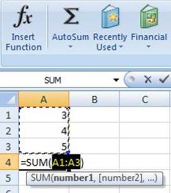
· AUTOSUM– This function allows you to enter formulas into a spreadsheet quickly and easily. With AUTOSUM, you won’t have to remember the syntax of any Excel function/formula. To use this function, you must:

13. Highlight the cell at the end of a row/column. For example, if you are working on A1, A2, A3, and A4, you should highlight A5.

14. Click on the ribbon named FORMULAS and hit AUTOSUM. Excel will highlight the entire row/column and display a pre-installed function in the empty cell.

15. If Excel highlighted the correct cells and provided the correct function, hit the Enter key. If there’s anything wrong with the automated process, make the necessary changes using the Formula Bar. Once done, press Enter.

Here’s a screenshot:

How to Use Other Functions

“SUM” serves as the default function of AUTOSUM. However, you can pick other functions easily. Once you click on the AUTOSUM button, Excel will show you several options such as MIN, MAX, AVERAGE, and COUNT NUMBERS. If you aren’t satisfied with these built-in functions, however, you may access Excel’s complete collection of functions. To see these functions, you must:

1. Highlight the cell where you want to place the result.

2. Access the ribbon named FORMULAS and hit INSERT FUNCTION. This is the first button of the ribbon.

3. A dialog box will appear on your screen. Here, you have two options:

1. First Option

1. Describe the function you want to use or choose a category from the dropdown menu.

2. The dialog box will show you several functions. Click on the one you want to use.

3. Excel will describe how the function works. Additionally, it will show you the syntax of that particular function.

4. If you want to learn more about that function, click on the blue link that says“Help on this function”.

5. Once you’re ready to use the function, hit the OK button.

6. Another dialog box will appear. This one, however, will suggest a group of cells where you can apply the function. If you want to use the suggested cells, just hit the Enter key. If the suggestion is incorrect, however, you may select the appropriate cells manually and hit Enter.

2. Second Option

1. Click on the button that says“Range Selector.” This action will give you a smaller dialog box.

2. Drag your mouse over the cells you want to work on.

3. Hit“Range Selector” again to go back to the previous dialog box.