Data Visualization with JavaScript (2015)
Chapter 6. Visualizing Geographic Data
Humans crave context when evaluating data, so it’s important to provide that context when it’s available. In the previous chapter, we saw how timelines can provide one frame of reference; now we’ll examine another equally important context: place. If a data set includes geographic coordinates or has values that correspond to different geographic regions, you can provide geographic context using a map-based visualization. The examples in this chapter consider two types of map-based visualizations.
In the first two examples, we want to show how data varies by region. The resulting visualizations, known as choropleth maps, use color to highlight different characteristics of the different regions. For the next two examples, the visualization data doesn’t itself vary by region directly, but the data does have a geographic component. By showing the data on a map, we can help our users understand it.
More specifically, we’ll see the following:
§ How to use special map fonts to create maps with minimal JavaScript
§ How to manipulate Scalable Vector Graphic (SVG) image maps with JavaScript
§ How to use a simple mapping library to add maps to web pages
§ How to integrate a full-featured map library into a visualization
Using Map Fonts
One technique for adding maps to web pages is surprisingly simple but often overlooked—map fonts. Two examples of these fonts are Stately (http://intridea.github.io/stately/) for the United States and Continental (http://contfont.net/) for Europe. Map fonts are special-purpose web fonts whose character sets contain map symbols instead of letters and numbers. In just a few easy steps, we’ll create a visualization of Europe using the symbols from Continental.
Step 1: Include the Fonts in the Page
The main websites for both Stately and Continental include more detailed instructions for installing the fonts, but all that’s really necessary is including a single CSS style sheet. In the case of Continental, that style sheet is called, naturally, continental.css. No JavaScript libraries are required.
<!DOCTYPE html>
<html lang="en">
<head>
<meta charset="utf-8">
<title></title>
<link rel="stylesheet" type="text/css" href="css/continental.css">
</head>
<body>
<div id="map"></div>
</body>
</html>
NOTE
For a production website, you might want to combine continental.css with your site’s other style sheets to minimize the number of network requests the browser has to make.
Step 2: Display One Country
To show a single country, all we have to do is include an HTML <span> element with the appropriate attributes. We can do this right in the markup, adding a class attribute set to map- followed by a two-letter country abbreviation. (fr is the international two-letter abbreviation for France.)
<div id="map">
<span class="map-fr"></span>
</div>
For this example, we’ll use JavaScript to generate the markup.
var fr = document.createElement("span");
fr.className = "map-fr";
document.getElementById("map").appendChild(fr);
Here we’ve created a new <span> element, giving it a class name of "map-fr", and appending it to the map <div>.
One last bit of housekeeping is setting the size of the font. By default, any map font character will be the same size as a regular text character. For maps we want something much larger, so we can use standard CSS rules to increase the size.
#map {
font-size: 200px;
}
That’s all it takes to add France to a web page, as you can see in Figure 6-1.
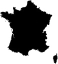
Figure 6-1. Map fonts make it very easy to add a map to a web page.
Step 3: Combine Multiple Countries into a Single Map
For this example we want to show more than a single country. We’d like to visualize the median age for all of Europe’s countries, based on United Nations population data (http://www.un.org/en/development/desa/population/) from 2010. To do that, we’ll create a map that includes all European countries, and we’ll style each country according to the data.
The first step in this visualization is putting all of the countries into a single map. Since each country is a separate character in the Continental font, we want to overlay those characters on top of one another rather than spread them across the page. That requires setting a couple of CSS rules.
#map {
➊ position: relative;
}
#map > [class*="map-"] {
➋ position: absolute;
➌ top: 0;
left: 0;
}
First we set the position of the outer container to relative ➊. This rule doesn’t change the styling of the outer container at all, but it does establish a positioning context for anything within the container. Those elements will be our individual country symbols, and we set their position to be absolute ➋. We then place each one at the top and left ➌, respectively, of the map so they’ll overlay one another. Because we’ve positioned the container relative, the country symbols will be positioned relative to that container rather than to the page as a whole.
Note that we’ve used a couple of CSS tricks to apply this positioning to all of the individual symbols within this element. We start by selecting the element with an id of map. Nothing fancy there. The direct descendent selector (>), however, says that what follows should match only elements that are immediate children of that element, not arbitrary descendants. Finally, the attribute selector [class*="map-"] specifies only children that have a class containing the characters map-. Since all the country symbols will be <span> elements with a class of map-xx (where xx is the two-letter country abbreviation), this will match all of our countries.
In our JavaScript, we can start with an array listing all of the countries and iterate through it. For each country, we create a <span> element with the appropriate class and insert it in the map <div>.
var countries = [
"ad", "al", "at", "ba", "be", "bg", "by", "ch", "cy", "cz",
"de", "dk", "ee", "es", "fi", "fo", "fr", "ge", "gg", "gr",
"hr", "hu", "ie", "im", "is", "it", "je", "li", "lt", "lu",
"lv", "mc", "md", "me", "mk", "mt", "nl", "no", "pl", "pt",
"ro", "rs", "ru", "se", "si", "sk", "sm", "tr", "ua", "uk",
"va"
];
var map = document.getElementById("map");
countries.forEach(function(cc) {
var span = document.createElement("span");
span.className = "map-" + cc;
map.appendChild(span);
});
With these style rules defined, inserting multiple <span> elements within our map <div> creates the complete, if somewhat uninteresting, map of Europe shown in Figure 6-2.
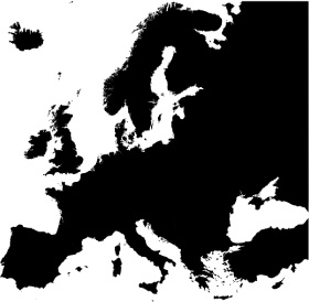
Figure 6-2. Overlaying map characters on top of one another creates a complete map.
Step 4: Vary the Countries Based on the Data
Now we’re ready to create the actual data visualization. Naturally, we’ll start with the data, in this case from the United Nations. Here’s how we could format that data in a JavaScript array. (The full data set can be found with the book’s source code at http://jsDataV.is/source/.)
var ages = [
{ "country": "al", "age": 29.968 },
{ "country": "at", "age": 41.768 },
{ "country": "ba", "age": 39.291 },
{ "country": "be", "age": 41.301 },
{ "country": "bg", "age": 41.731 },
// Data set continues...
There are several ways we could use this data to modify the map. We could use JavaScript code to set the visualization properties directly by, for example, changing the color style for each country symbol. That would work, but it forgoes one of the big advantages of map fonts. With map fonts, our visualization is standard HTML, so we can use standard CSS to style it. If, in the future, we want to change the styles on the page, they’ll all be contained within the style sheets, and we won’t have to hunt through our JavaScript code to adjust colors.
To indicate which styles are appropriate for an individual country symbol, we can attach a data- attribute to each.
➊ var findCountryIndex = function(cc) {
for (var idx=0; idx<ages.length; idx++) {
if (ages[idx].country === cc) {
return idx;
}
}
return -1;
}
var map = document.getElementById("map");
countries.forEach(function(cc) {
var idx = findCountryIndex(cc);
if (idx !== -1) {
var span = document.createElement("span");
span.className = "map-" + cc;
➋ span.setAttribute("data-age", Math.round(ages[idx].age));
map.appendChild(span);
}
});
In this code, we set the data-age attribute to the mean age, rounded to the nearest whole number ➋. To find the age for a given country, we need that country’s index in the ages array. The findCountryIndex() function ➊ does that in a straightforward way.
Now we can assign CSS style rules based on that data-age attribute. Here’s the start of a simple blue gradient for the different ages, where greater median ages are colored darker blue-green.
#map > [data-age="44"] { color: #2d9999; }
#map > [data-age="43"] { color: #2a9493; }
#map > [data-age="42"] { color: #278f8e; }
/* CSS rules continue... */
NOTE
Although they’re beyond the scope of this book, CSS preprocessors such as LESS (http://lesscss.org/) and SASS (http://sass-lang.com/) make it easy to create these kinds of rules.
Now we have the nice visualization of the age trends shown in Figure 6-3.
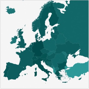
Figure 6-3. With CSS rules, we can change the styles of individual map symbols.
Step 5: Add a Legend
To finish off the visualization, we can add a legend to the map. Because the map itself is nothing more than standard HTML elements with CSS styling, it’s easy to create a matching legend. This example covers a fairly broad range (ages 28 to 44), so a linear gradient works well as a key. Your own implementation will depend on the specific browser versions that you wish to support, but a generic style rule would be as follows:
#map-legend .key {
background: linear-gradient(to bottom, #004a4a 0%,#2d9999 100%);
}
The resulting visualization in Figure 6-4 summarizes the median age for European countries in a clear and concise format.
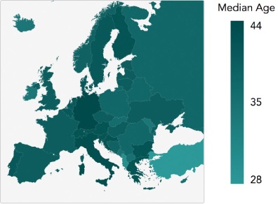
Figure 6-4. Standard HTML can also provide a legend for the visualization.
Working with Scalable Vector Graphics
Map fonts like those in the previous example are easy to use and visually effective, but only a few map fonts exist, and they definitely don’t cover all the conceivable geographic regions. For visualizations of other regions, we’ll have to find a different technique. Maps, of course, are ultimately images, and web browsers can display many different image formats. One format in particular, called Scalable Vector Graphics (SVG), is especially well suited for interactive visualizations. That’s because, as we’ll see in this example, JavaScript code (as well as CSS styles) can easily and naturally interact with SVG images.
Although our example for this section deals with a map, the techniques here are by no means limited to maps. Whenever you have a diagram or illustration in SVG format, you can manipulate it directly on a web page.
NOTE
There is one important consideration for using SVG: only modern web browsers support it. more specifically, IE8 (and earlier) cannot display SVG images. If a significant number of your users are using older browsers, you might want to consider alternatives.
For web developers, SVG is especially convenient because its syntax uses the same structure as HTML. You can use many of the same tools and techniques for working with HTML on SVG as well. Consider, for example, a skeletal HTML document.
<!DOCTYPE html>
<html lang="en">
<head><!-- --></head>
<body>
<nav><!-- --></nav>
<main>
<section><!-- --></section>
</main>
<nav><!-- --></nav>
</body>
</html>
Compare that to the next example: the universal symbol for first aid represented in an SVG document.
NOTE
If you have worked with htmL before htmL5, the similarities might be especially striking, as the SVG header text follows the same format as htmL4.
<?xml version="1.0" encoding="UTF-8"?>
<!DOCTYPE svg PUBLIC "-//W3C//DTD SVG 1.1//EN"
"http://www.w3.org/Graphics/SVG/1.1/DTD/svg11.dtd">
<svg id="firstaid" version="1.1" xmlns="http://www.w3.org/2000/svg"
width="100" height="100">
<rect id="background" x="0" y="0" width="100" height="100" rx="20" />
<rect id="vertical" x="39" y="19" width="22" height="62" />
<rect id="horizontal" x="19" y="39" width="62" height="22" />
</svg>
You can even style the SVG elements using CSS. Here’s how we could color the preceding image:
svg#firstaid {
stroke: none;
}
svg#firstaid #background {
fill: #000;
}
svg#firstaid #vertical,
svg#firstaid #horizontal {
fill: #FFF;
}
Figure 6-5 shows how that SVG renders.

Figure 6-5. SVG images may be embedded directly within web pages.
The affinity between HTML and SVG is, in fact, far stronger than the similar syntax. With modern browsers, you can mix SVG and HTML in the same web page. To see how that works, let’s visualize health data for the 159 counties in the US state of Georgia. The data comes from County Health Rankings (http://www.countyhealthrankings.org/).
Step 1: Create the SVG Map
Our visualization starts with a map, so we’ll need an illustration of Georgia’s counties in SVG format. Although that might seem like a challenge, there are actually many sources for SVG maps that are free to use, as well as special-purpose applications that can generate SVG maps for almost any region. The Wikimedia Commons (http://commons.wikimedia.org/wiki/Main_Page), for example, contains a large number of open source maps, including many of Georgia. We’ll use one showing data from the National Register of Historic Places (http://commons.wikimedia.org/wiki/File:NRHP_Georgia_Map.svg#file).
After downloading the map file, we can adjust it to better fit our needs, removing the legend, colors, and other elements that we don’t need. Although you can do this in a text editor (just as you can edit HTML), you may find it easier to use a graphics program such as Adobe Illustrator or a more web-focused app like Sketch (http://www.bohemiancoding.com/sketch/). You might also want to take advantage of an SVG optimization website (http://petercollingridge.appspot.com/svg-optimiser/) or application (https://github.com/svg/), which can compress an SVG by removing extraneous tags and reducing the sometimes-excessive precision of graphics programs.
Our result will be a series of <path> elements, one for each county. We’ll also want to assign a class or id to each path to indicate the county. The resulting SVG file might begin like the following.
<svg version="1.1" xmlns="http://www.w3.org/2000/svg"
width="497" height="558">
<path id="ck" d="M 216.65,131.53 L 216.41,131.53 216.17,131.53..." />
<path id="me" d="M 74.32,234.01 L 74.32,232.09 74.32,231.61..." />
<path id="ms" d="M 64.96,319.22 L 64.72,319.22 64.48,318.98..." />
<!-- Markup continues... -->
To summarize, here are the steps to create the SVG map.
1. Locate a suitably licensed SVG-format map file or create one using a special-purpose map application.
2. Edit the SVG file in a graphics application to remove extraneous components and simplify the illustration.
3. Optimize the SVG file using an optimization site or application.
4. Make final adjustments (such as adding id attributes) in your regular HTML editor.
Step 2: Embed the Map in the Page
The simplest way to include an SVG map in a web page is to embed the SVG markup directly within the HTML markup. To include the first-aid symbol, for example, just include the SVG tags within the page itself, as shown at ➊ through ➋. You don’t have to include the header tags that are normally present in a standalone SVG file.
<!DOCTYPE html>
<html lang="en">
<head>
<meta charset="utf-8">
<title></title>
</head>
<body>
<div>
➊ <svg id="firstaid" version="1.1"
xmlns="http://www.w3.org/2000/svg"
width="100" height="100">
<rect id="background" x="0" y="0"
width="100" height="100" rx="20" />
<rect id="vertical" x="39" y="19"
width="22" height="62" />
<rect id="horizontal" x="19" y="39"
width="62" height="22" />
➋ </svg>
</div>
</body>
</html>
If your map is relatively simple, direct embedding is the easiest way to include it in the page. Our map of Georgia, however, is about 1 MB even after optimization. That’s not unusual for maps with reasonable resolution, as describing complex borders such as coastlines or rivers can make for large <path> elements. Especially if the map isn’t the sole focus of the page, you can provide a better user experience by loading the rest of the page first. That will give your users something to read while the map loads in the background. You can even add a simple animated progress loader if that’s appropriate for your site.
If you’re using jQuery, loading the map is a single instruction. You do want to make sure, though, that your code doesn’t start manipulating the map until the load is complete. Here’s how that would look in the source code.
$("#map").load("img/ga.svg", function() {
// Only manipulate the map inside this block
})
Step 3: Collect the Data
The data for our visualization is available as an Excel spreadsheet directly from County Health Rankings (http://www.countyhealthrankings.org/). We’ll convert that to a JavaScript object in advance, and we’ll add a two-letter code corresponding to each county. Here’s how that array might begin.
var counties = [
{
"name":"Appling",
"code":"ap",
"outcomes_z":0.93,
"outcomes_rank":148,
// Data continues...
},
{
"name":"Atkinson",
"code":"at",
"outcomes_z":0.40,
"outcomes_rank":118,
// Data set continues...
];
For this visualization we’d like to show the variation in health outcomes among counties. The data set provides two variables for that value, a ranking and a z-score (a measure of how far a sample is from the mean in terms of standard deviation). The County Health Rankings site provides z-scores slightly modified from the traditional statistical definition. Normal z-scores are always positive; in this data set, however, measurements that are subjectively better than average are multiplied by –1 so that they are negative. A county whose health outcome is two standard deviations “better” than the mean, for example, is given a z-score of –2 instead of 2. This adjustment makes it easier to use these z-scores in our visualization.
Our first step in working with these z-scores is to find the maximum and minimum values. We can do that by extracting the outcomes as a separate array and then using JavaScript’s built-in Math.max() and Math.min() functions. Note that the following code uses the map() method to extract the array, and that method is available only in modern browsers. Since we’ve chosen to use SVG images, however, we’ve already restricted our users to modern browsers, so we might as well take advantage of that when we can.
var outcomes = counties.map(function(county) {return county.outcomes_z;});
var maxZ = Math.max.apply(null, outcomes);
var minZ = Math.min.apply(null, outcomes);
Notice how we’ve used the .apply() method here. Normally the Math.max() and Math.min() functions accept a comma-separated list of arguments. We, of course, have an array instead. The apply() method, which works with any JavaScript function, turns an array into a comma-separated list. The first parameter is the context to use, which in our case doesn’t matter, so we set it to null.
To complete the data preparation, let’s make sure the minimum and maximum ranges are symmetric about the mean.
if (Math.abs(minZ) > Math.abs(maxZ)) {
maxZ = -minZ;
} else {
minZ = -maxZ;
}
If, for example, the z-scores ranged from -2 to 1.5, this code would extend the range to [-2, 2]. This adjustment will make the color scales symmetric as well, thus making our visualization easier for users to interpret.
Step 4: Define the Color Scheme
Defining an effective color scheme for a map can be quite tricky, but fortunately there are some excellent resources available. For this visualization we’ll rely on the Chroma.js library (http://driven-by-data.net/about/chromajs/). That library includes many tools for working with and manipulating colors and color scales, and it can satisfy the most advanced color theorist. For our example, however, we can take advantage of the predefined color scales, specifically those defined originally by Cynthia Brewer (http://colorbrewer2.org/).
The Chroma.js library is available on popular content distribution networks, so we can rely on a network such as CloudFlare’s cdnjs (http://cdnjs.com/) to host it.
<!DOCTYPE html>
<html lang="en">
<head>
<meta charset="utf-8">
<title></title>
</head>
<body>
<div id="map"></div>
<script
src="///cdnjs.cloudflare.com/ajax/libs/chroma-js/0.5.2/chroma.min.js">
</script>
</body>
</html>
To use a predefined scale, we pass the scale’s name ("BrBG" for Brewer’s brown-to-blue-green scale) to the chroma.scale() function.
var scale = chroma.scale("BrBG").domain([maxZ, minZ]).out("hex");
At the same time, we indicate the domain for our scale (minZ to maxZ, although we’re reversing the order because of the data set’s z-score adjustment) and our desired output. The "hex" output is the common "#012345" format compatible with CSS and HTML markup.
Step 5: Color the Map
With our color scheme established, we can now apply the appropriate colors to each county on the map. That’s probably the easiest step in the whole visualization. We iterate through all the counties, finding their <path> elements based on their id values, and applying the color by setting the fill attribute.
counties.forEach(function(county) {
document.getElementById(county.code)
.setAttribute("fill", scale(county.outcomes_z));
})
The resulting map, shown in Figure 6-6, illustrates which counties are above average and which are below average for health outcomes in 2014.
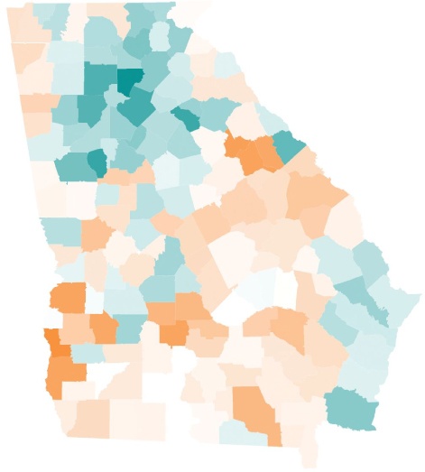
Figure 6-6. CSS rules can set the styles for individual SVG elements within an SVG illustration.
Step 6: Add a Legend
To help users interpret the map, we can add a legend to the visualization. We can take advantage of the Chroma.js scale to easily create a table that explains the variation. For the table, we’ll use four increments for the colors on each side of the mean value. That gives us a total of nine colors for the legend.
<table id="legend">
<tr class="scale">
<td></td><td></td><td></td><td></td><td></td>
<td></td><td></td><td></td><td></td>
</tr>
<tr class="text">
<td colspan="4">Worse than Average</td>
<td>Average</td>
<td colspan="4">Better than Average</td>
</tr>
</table>
Some straightforward CSS will style the table appropriately. Because we have nine colors, we set the width of each table cell to 11.1111% (1/9 is 0.111111).
table#legend tr.scale td {
height: 1em;
width: 11.1111%;
}
table#legend tr.text td:first-child {
text-align: left;
}
table#legend tr.text td:nth-child(2) {
text-align: center;
}
table#legend tr.text td:last-child {
text-align: right;
}
Finally, we use the Chroma scale created earlier to set the background color for the legend’s table cells. Because the legend is a <table> element, we can directly access the rows and the cells within the rows. Although these elements look like arrays in the following code, they’re not true JavaScript arrays, so they don’t support array methods such as forEach(). For now, we’ll iterate through them with a for loop, but if you’d rather use the array methods, stay tuned for a simple trick. Note that once again we’re working backward because of the data set’s z-score adjustments.
var legend = document.getElementById("legend");
var cells = legend.rows[0].cells;
for (var idx=0; idx<cells.length; idx++) {
var td = cells[idx];
➊ td.style.backgroundColor = scale(maxZ -
((idx + 0.5) / cells.length) * (maxZ - minZ));
};
At ➊ we calculate the fraction of the current index from the total number of legend colors ((idx + 0.5) / cells.length), multiply that by the total range of the scale (maxZ - minZ), and subtract the result from the maximum value.
The result is the legend for the map in Figure 6-7.

Figure 6-7. An HTML <table> can serve as a legend.
Step 7: Add Interactions
To complete the visualization, let’s enable users to hover their mouse over a county on the map to see more details. Of course, mouse interactions are not available for tablet or smartphone users. To support those users, you could add a similar interaction for tap or click events. That code would be almost identical to the next example.
We’ll start by defining a table to show county details.
<table id="details">
<tr><td>County:</td><td></td></tr>
<tr><td>Rank:</td><td></td></tr>
<tr><td>Health Behaviors:</td><td></td></tr>
<tr><td>Clinical Care:</td><td></td></tr>
<tr><td>Social & Economic Factors:</td><td></td></tr>
<tr><td>Physical Environment:</td><td></td></tr>
</table>
Initially, we don’t want that table to be visible.
table#details {
display: none;
}
To show the table, we use event handler functions that track when the mouse enters or leaves an SVG path for a county. To find these <path> elements, we can use the querySelectorAll() function that modern browsers support. Unfortunately, that function doesn’t return a true array of elements, so we can’t use array methods such as forEach() to iterate through those elements. There’s a trick, however, that will let us convert the returned list into a true array.
[].slice.call(document.querySelectorAll("#map path"))
.forEach(function(path) {
path.addEventListener("mouseenter", function(){
document.getElementById("details").style.display = "table";
});
path.addEventListener("mouseleave", function(){
document.getElementById("details").style.display = "none";
});
}
);
This code calls the [].slice.call() function with the “not quite array” object as its parameter. The result is a true array with all of its useful methods.
In addition to making the details table visible, we’ll also want to update it with the appropriate information. To help with this display, we can write a function that converts a z-score into a more user-friendly explanation. The specific values in the following example are arbitrary since we’re not trying for statistical precision in this visualization.
var zToText = function(z) {
z = +z;
if (z > 0.25) { return "Far Below Average"; }
if (z > 0.1) { return "Below Average"; }
if (z > -0.1) { return "Average"; }
if (z > -0.25) { return "Above Average"; }
return "Far Above Average";
}
There are a couple of noteworthy items in this function. First, the statement z = +z converts the z-score from a string to a numeric value for the tests that follow. Second, remember that because of the z-score adjustments, the negative z-scores are actually better than average, while the positive values are below average.
We can use this function to provide the data for our details table. The first step is finding the full data set for the associated <path> element. To do that, we search through the counties array looking for a code property that matches the id attribute of the path.
var county = null;
counties.some(function(c) {
if (c.code === this.id) {
county = c;
return true;
}
return false;
});
Because indexOf() doesn’t allow us to find objects by key, we’ve used the some() method instead. That method terminates as soon as it finds a match, so we avoid iterating through the entire array.
Once we’ve found the county data, it’s a straightforward process to update the table. The following code directly updates the relevant table cell’s text content. For a more robust implementation, you could provide class names for the cells and update based on those class names.
var table = document.getElementById("details");
table.rows[0].cells[1].textContent =
county.name;
table.rows[1].cells[1].textContent =
county.outcomes_rank + " out of " + counties.length;
table.rows[2].cells[1].textContent =
zToText(county.health_behaviors_z);
table.rows[3].cells[1].textContent =
zToText(county.clinical_care_z);
table.rows[4].cells[1].textContent =
zToText(county.social_and_economic_factors_z);
table.rows[5].cells[1].textContent =
zToText(county.physical_environment_z);
Now we just need a few more refinements:
path.addEventListener("mouseleave", function(){
// Previous code
➊ this.setAttribute("stroke", "#444444");
});
path.addEventListener("mouseleave", function(){
// Previous code
➋ this.setAttribute("stroke", "none");
});
Here we add a stroke color at ➊ for counties that are highlighted. We remove the stroke at ➋ when the mouse leaves the path.
At this point our visualization example is complete. Figure 6-8 shows the result.
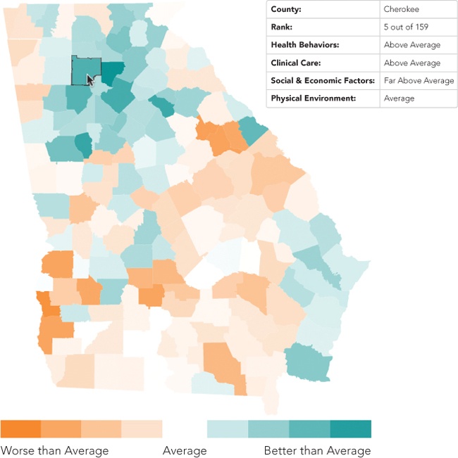
Figure 6-8. Browsers (and a bit of code) can turn SVG illustrations into interactive visualizations.
Including Maps for Context
So far in this chapter, we’ve looked at map visualizations where the main subjects are geographic regions—countries in Europe or counties in Georgia. In those cases, choropleth maps were effective in showing the differences between regions. Not all map visualizations have the same focus, however. In some cases, we want to include a map more as context or background for the visualization data.
When we want to include a map as a visualization background, we’re likely to find that traditional mapping libraries will serve us better than custom choropleth maps. The most well-known mapping library is probably Google Maps (http://maps.google.com/), and you’ve almost certainly seen many examples of embedded Google maps on web pages. There are, however, several free and open source alternatives to Google Maps. For this example, we’ll use the Modest Maps library (https://github.com/modestmaps/modestmaps-js/) from Stamen Design. To show off this library, we’ll visualize the major UFO sightings in the United States (http://en.wikipedia.org/wiki/UFO_sightings_in_the_United_States), or at least those important enough to merit a Wikipedia entry.
Step 1: Set Up the Web Page
For our visualization, we’ll rely on a couple of components from the Modest Maps library: the core library itself and the spotlight extension that can be found in the library’s examples folder. In production you would likely combine these and minify the result to optimize performance, but for our example, we’ll include them separately.
<!DOCTYPE html>
<html lang="en">
<head>
<meta charset="utf-8">
<title></title>
</head>
<body>
➊ <div id="map"></div>
<script src="js/modestmaps.js"></script>
<script src="js/spotlight.js"></script>
</body>
</html>
We’ve also set aside a <div> at ➊ to hold the map. Not surprisingly, it has the id of "map".
Step 2: Prepare the Data
The Wikipedia data can be formatted as an array of JavaScript objects. We can include whatever information we wish in the objects, but we’ll definitely need the latitude and longitude of the sighting in order to place it on the map. Here’s how you might structure the data.
var ufos = [
{
"date": "April, 1941",
"city": "Cape Girardeau",
"state": "Missouri",
"location": [37.309167, -89.546389],
"url": "http://en.wikipedia.org/wiki/Cape_Girardeau_UFO_crash"
},{
"date": "February 24, 1942",
"city": "Los Angeles",
"state": "California",
"location": [34.05, -118.25],
"url": "http://en.wikipedia.org/wiki/Battle_of_Los_Angeles"
},{
// Data set continues...
The location property holds the latitude and longitude (where negative values indicate west) as a two-element array.
Step 3: Choose a Map Style
As with most mapping libraries, Modest Maps builds its maps using layers. The layering process works much like it does in a graphics application such as Photoshop or Sketch. Subsequent layers add further visual information to the map. In most cases, the base layer for a map consists of image tiles. Additional layers such as markers or routes can be included on top of the image tiles.
When we tell Modest Maps to create a map, it calculates which tiles (both size and location) are needed and then it requests those tiles asynchronously over the Internet. The tiles define the visual style of the map. Stamen Design has published several tile sets itself; you can see them on http://maps.stamen.com/.
To use the Stamen tiles, we’ll add one more, small JavaScript library to our page. That library is available directly from Stamen Design (http://maps.stamen.com/js/tile.stamen.js). It should be included after the Modest Maps library.
<!DOCTYPE html>
<html lang="en">
<head>
<meta charset="utf-8">
<title></title>
</head>
<body>
<div id="map"></div>
<script src="js/modestmaps.js"></script>
<script src="js/spotlight.js"></script>
<script src="http://maps.stamen.com/js/tile.stamen.js"></script>
</body>
</html>
For our example, the “toner” style is a good match, so we’ll use those tiles. To use those tiles, we create a tile layer for the map.
var tiles = new MM.StamenTileLayer("toner");
When you consider a source for image tiles, be aware of any copyright restrictions. Some image tiles must be licensed, and even those that are freely available often require that any user identify the provider as the source.
Step 4: Draw the Map
Now we’re ready to draw the map itself. That takes two JavaScript statements:
var map = new MM.Map("map", tiles);
map.setCenterZoom(new MM.Location(38.840278, -96.611389), 4);
First we create a new MM.Map object, giving it the id of the element containing the map and the tiles we just initialized. Then we provide the latitude and longitude for the map’s center as well as an initial zoom level. For your own maps, you may need to experiment a bit to get the right values, but for this example, we’ll center and zoom the map so that it comfortably shows the continental United States.
The resulting map, shown in Figure 6-9, forms a base for showing the sightings.
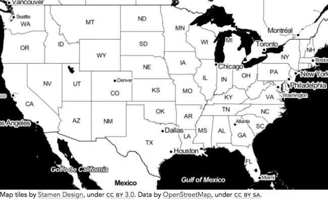
Figure 6-9. Map libraries can show maps based on geographic coordinates.
Notice that both Stamen Design and OpenStreetMap are credited. That attribution is required by the terms of the Stamen Design license.
Step 5: Add the Sightings
With our map in place, it’s time to add the individual UFO sightings. We’re using the spotlight extension to highlight these locations, so we first create a spotlight layer for the map. We’ll also want to set the radius of the spotlight effect. As with the center and zoom parameters, a bit of trial and error helps here.
var layer = new SpotlightLayer();
layer.spotlight.radius = 15;
map.addLayer(layer);
Now we can iterate through the array of sightings that make up our data. For each sighting, we extract the latitude and longitude of the location and add that location to the spotlight layer.
ufos.forEach(function(ufo) {
layer.addLocation(new MM.Location(ufo.location[0], ufo.location[1]));
});
At this point our visualization is complete. Figure 6-10 shows where UFOs have allegedly appeared over the United States in a suitably mysterious context.
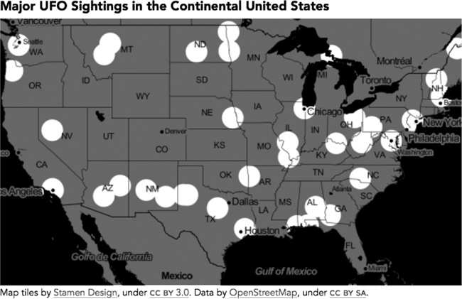
Figure 6-10. Adding layers in a map library can emphasize regions of a map.
Integrating a Full-Featured Mapping Library
The Modest Maps library of the previous example is a fine library for simple map visualizations, but it doesn’t have all of the features and support of a full-featured service such as Google Maps. There is, however, an open source library that does provide those features: Leaflet (http://leafletjs.com/). In this example, we’ll build a more complex visualization that features a Leaflet-based map.
In the 1940s, two private railroads were in competition for passenger traffic in the southeastern United States. Two routes that competed most directly were the Silver Comet (run by Seaboard Air Lines) and the Southerner (operated by Southern Railways). Both served passengers traveling between New York and Birmingham, Alabama. One factor cited in the Southerner’s ultimate success was the shorter distance of its route. Trips on the Southerner were quicker, giving Southern Railways a competitive advantage. Let’s create a visualization to demonstrate that advantage.
Step 1: Prepare the Data
The data for our visualization is readily available as timetables for the two routes. A more precise comparison might consider timetables from the same year, but for this example, we’ll use the Southerner’s timetable from 1941 (http://www.streamlinerschedules.com/concourse/track1/southerner194112.html) and the Silver Comet’s timetable from 1947 (http://www.streamlinerschedules.com/concourse/track1/silvercomet194706.html), as they are readily available on the Internet. The timetables only include station names, so we will have to look up latitude and longitude values (using, for example, Google Maps) for all of the stations in order to place them on a map. We can also calculate the time difference between stops, in minutes. Those calculations result in two arrays, one for each train.
var seaboard = [
{ "stop": "Washington",
"latitude": 38.895111, "longitude": -77.036667,
"duration": 77 },
{ "stop": "Fredericksburg",
"latitude": 38.301806, "longitude": -77.470833,
"duration": 89 },
{ "stop": "Richmond",
"latitude": 37.533333, "longitude": -77.466667,
"duration": 29 },
// Data set continues...
];
var southern = [
{ "stop": "Washington",
"latitude": 38.895111, "longitude": -77.036667,
"duration": 14 },
{ "stop": "Alexandria",
"latitude": 38.804722, "longitude": -77.047222,
"duration": 116 },
{ "stop": "Charlottesville",
"latitude": 38.0299, "longitude": -78.479,
"duration": 77 },
// Data set continues...
];
Step 2: Set Up the Web Page and Libraries
To add Leaflet maps to our web page, we’ll need to include the library and its companion style sheet. Both are available from a content distribution network, so there’s no need to host them on our own servers.
<!DOCTYPE html>
<html lang="en">
<head>
<meta charset="utf-8">
<title></title>
<link rel="stylesheet"
href="http://cdn.leafletjs.com/leaflet-0.7.2/leaflet.css" />
</head>
<body>
➊ <div id="map"></div>
<script
src="http://cdn.leafletjs.com/leaflet-0.7.2/leaflet.js">
</script>
</body>
</html>
When we create our page, we also define a <div> container for the map at ➊.
Step 3: Draw the Base Map
The Silver Comet and the Southerner traveled between New York and Birmingham (and, in the case of the Southerner, all the way to New Orleans). But the region that’s relevant for our visualization lies between Washington, DC, and Atlanta, Georgia, because that’s the only region where the train routes differed; for the rest of their journeys, the routes were essentially the same. Our map, therefore, will extend from Atlanta in the southwest to Washington, DC, in the northeast. Using a bit of trial and error, we can determine the best center point and zoom level for the map. The center point defines the latitude and longitude for the map’s center, and the zoom level determines the area covered by the map on its initial display. When we create the map object, we give it the id of the containing element as well as those parameters.
var map = L.map("map",{
center: [36.3, -80.2],
zoom: 6
});
For this particular visualization, there is little point in zooming or panning the map, so we can include additional options to disable those interactions.
var map = L.map("map",{
center: [36.3, -80.2],
➊ maxBounds: [ [33.32134852669881, -85.20996093749999],
➋ [39.16414104768742, -75.9814453125] ],
zoom: 6,
➌ minZoom: 6,
➍ maxZoom: 6,
➎ dragging: false,
➏ zoomControl: false,
➐ touchZoom: false,
scrollWheelZoom: false,
doubleClickZoom: false,
➑ boxZoom: false,
➒ keyboard: false
});
Setting both the minimum zoom level ➌ and the maximum zoom level ➍ to be equal to the initial zoom level disables zooming. We also disable the onscreen map controls for zooming at ➏. The other zoom controls are likewise disabled (➐ through ➑). For panning, we disable dragging the map at ➎ and keyboard arrow keys at ➒. We also specify the latitude/longitude bounds for the map (➊ and ➋).
Because we’ve disabled the user’s ability to pan or zoom the map, we should also make sure the mouse cursor doesn’t mislead the user when it’s hovering over the map. The leaflet.css style sheet expects zooming and panning to be enabled, so it sets the cursor to a “grabbing” hand icon. We can override that value with a style rule of our own. We have to define this rule after including the leaflet.css file.
.leaflet-container {
cursor: default;
}
As with the Modest Maps example, we base our map on a set of tiles. There are many tile providers that support Leaflet; some are open source, while others are commercial. Leaflet has a demo page (http://leaflet-extras.github.io/leaflet-providers/preview/) you can use to compare some of the open source tile providers. For our example, we want to avoid tiles with roads, as the highway network looked very different in the 1940s. Esri has a neutral WorldGrayCanvas set that works well for our visualization. It does include current county boundaries, and some counties may have changed their borders since the 1940s. For our example, we won’t worry about that detail, though you might consider it in any production visualization. Leaflet’s API lets us create the tile layer and add it to the map in a single statement. The Leaflet includes a built-in option to handle attribution so we can be sure to credit the tile source appropriately.
L.tileLayer("http://server.arcgisonline.com/ArcGIS/rest/services/"+
"Canvas/World_Light_Gray_Base/MapServer/tile/{z}/{y}/{x}", {
attribution: "Tiles © Esri — Esri, DeLorme, NAVTEQ",
➊ maxZoom: 16
}).addTo(map);
Note that the maxZoom option at ➊ indicates the maximum zoom layer available for that particular tile set. That value is independent of the zoom level we’re permitting for our map.
With a map and a base tile layer, we have a good starting point for our visualization in (see Figure 6-11).
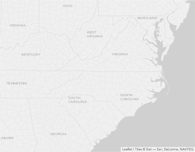
Figure 6-11. A base layer map provides the canvas for a visualization.
Step 4: Add the Routes to the Map
For the next step in our visualization, we want to show the two routes on our map. First, we’ll simply draw each route on the map. Then, we’ll add an animation that traces both routes at the same time to show which one is faster.
The Leaflet library includes a function that does exactly what we need to draw each route: polyline() connects a series of lines defined by the latitude and longitude of their endpoints and prepares them for a map. Our data set includes the geographic coordinates of each route’s stops, so we can use the JavaScript map() method to format those values for Leaflet. For the Silver Comet example, the following statement extracts its stops.
seaboard.map(function(stop) {
return [stop.latitude, stop.longitude]
})
This statement returns an array of latitude/longitude pairs:
[
[38.895111,-77.036667],
[38.301806,-77.470833],
[37.533333,-77.466667],
[37.21295,-77.400417],
/* Data set continues... */
]
That result is the perfect input to the polyline() function. We’ll use it for each of the routes. The options let us specify a color for the lines, which we’ll match with the associated railroad’s official color from the era. We also indicate that the lines have no function when clicked by setting the clickable option to false.
L.polyline(
seaboard.map(function(stop) {return [stop.latitude, stop.longitude]}),
{color: "#88020B", weight: 1, clickable: false}
).addTo(map);
L.polyline(
southern.map(function(stop) {return [stop.latitude, stop.longitude]}),
{color: "#106634", weight: 1, clickable: false}
).addTo(map);
With this addition, the visualization shown in Figure 6-12 is starting to convey the relative distances of the two routes.
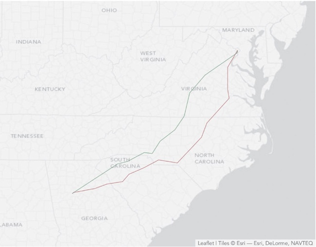
Figure 6-12. Additional map layers add data to the canvas.
Step 5: Add an Animation Control
Next, we’ll animate the two routes. Not only will this emphasize the competitive advantage of the shorter route, but it will also make the visualization more interesting and engaging. We’ll definitely want to let our users start and stop the animation, so our map will need a control button. The Leaflet library doesn’t have its own animation control, but the library does have a lot of support for customizations. Part of that support is a generic Control object. We can create an animation control by starting with that object and extending it.
L.Control.Animate = L.Control.extend({
// Custom code goes here
});
Next we define the options for our custom control. Those options include its position on the map, the text and tool tip (title) for its states, and functions to call when the animation starts or stops. We define these within an options object as follows, which lets Leaflet integrate them within its normal functionality.
L.Control.Animate = L.Control.extend({
options: {
position: "topleft",
animateStartText: "![]() ",
",
animateStartTitle: "Start Animation",
animatePauseText: "![]() ",
",
animatePauseTitle: "Pause Animation",
animateResumeText: "![]() ",
",
animateResumeTitle: "Resume Animation",
animateStartFn: null,
animateStopFn: null
},
For our example, we’re using UTF-8 characters for the play and pause control. In a production visualization, you might consider using icon fonts or images to have maximum control over the appearance.
Our animation control also needs an onAdd() method for Leaflet to call when it adds a control to a map. This method constructs the HTML markup for the control and returns that to the caller.
onAdd: function () {
var animateName = "leaflet-control-animate",
➊ container = L.DomUtil.create(
"div", animateName + " leaflet-bar"),
options = this.options;
➋ this._button = this._createButton(
this.options.animateStartText,
this.options.animateStartTitle,
animateName,
container,
this._clicked);
return container;
},
Our implementation of onAdd() constructs the markup in two stages. First, starting at ➊, it creates a <div> element and gives that element two classes: leaflet-control-animate and leaflet-bar. The first class is unique to our animation control, and we can use it to apply CSS rules uniquely to our control. The second class is a general Leaflet class for all toolbars. By adding it to the animation control, we’re making that control consistent with other Leaflet controls. Note that Leaflet includes the L.DomUtil.create() method at ➊ to handle the details of creating the element.
The second part of onAdd() creates a button element within this <div> container. Most of the work takes place in the _createButton() function at ➋, which we’ll examine shortly. The parameters to the function include the following:
§ The text for the button
§ The tool tip (title) to display when the mouse hovers over the button
§ The CSS class to apply to the button
§ The container in which to insert the button
§ A function to call when the button is clicked
If you’re wondering why the name of this function begins with an underscore (_), that’s the convention that Leaflet uses for private methods (and attributes). There’s no requirement to follow it, but doing so will make it easier for someone familiar with Leaflet to understand our code.
The _createButton() method itself relies on Leaflet utility functions.
_createButton: function (html, title, className, container, callback) {
➊ var link = L.DomUtil.create("a", className, container);
link.innerHTML = html;
link.href = "#";
➋ link.title = title;
L.DomEvent
➌ .on(link, "mousedown dblclick", L.DomEvent.stopPropagation)
➍ .on(link, "click", L.DomEvent.stop)
➎ .on(link, "click", callback, this);
return link;
},
First it creates the button as an <a> element with the specified text, title, and class, and it creates that element within the appropriate container (➊ through ➋). It then binds several events to this <a> element. First it ignores initial mousedown and double-click events at ➌. It also prevents single-click events from propagating up the document tree and from implementing their default behavior at ➍. Finally, it executes the callback function on click events at ➎.
The callback function itself is our next task.
➊ _running: false,
_clicked: function() {
➋ if (this._running) {
if (this.options.animateStopFn) {
this.options.animateStopFn();
}
this._button.innerHTML = this.options.animateResumeText;
this._button.title = this.options.animateResumeTitle;
} else {
if (this.options.animateStartFn) {
this.options.animateStartFn();
}
this._button.innerHTML = this.options.animatePauseText;
this._button.title = this.options.animatePauseTitle;
}
this._running = !this._running;
},
Before we get into the function, we add a single state variable (_running) to keep track of whether the animation is currently running. It starts out stopped at ➊. Then our callback function starts by checking this variable at ➋. If _running is true, that means the animation was running and has just been paused by the current click, so it changes the control to indicate that clicking will now resume the animation. If the animation isn’t running, the callback function does the opposite: it changes the control to indicate that a subsequent click will pause it. In both cases, the callback function executes the appropriate control function if one exists. Finally, it sets the state of _running to its complement.
The last part of our custom control adds a reset() method to clear the animation. This function sets the control back to its initial state.
reset: function() {
this._running = false;
this._button.innerHTML = this.options.animateStartText;
this._button.title = this.options.animateStartTitle;
}
});
To completely integrate our custom control into the Leaflet architecture, we add a function to the L.control object. Following the Leaflet convention, this function’s name begins with a lowercase letter but is otherwise identical to the name of our control.
L.control.animate = function (options) {
return new L.Control.Animate(options);
};
Defining this last function lets us create the control using a common Leaflet syntax.
L.control.animate().addTo(map);
This is the same syntax we’ve seen before with layers and polylines.
Step 6: Prepare the Animation
With a convenient user control in place, we can now begin work on the animation itself. Although this particular animation isn’t especially taxing, we can still follow best practices and compute as much as possible in advance. Since we’re animating two routes, we’ll define a function that will build an animation for any input route. A second parameter will specify polyline options. This function will return an array of polyline paths, indexed by minutes. You can see the basic structure of this function next.
var buildAnimation = function(route, options) {
var animation = [];
// Code to build the polylines
return animation;
}
The first element in the array will be the polyline for the first minute of the route. We’ll build the entire array in the animation variable.
To build the paths, we iterate through the stops on the route.
➊ for (var stopIdx=0, prevStops=[];
stopIdx < route.length-1; stopIdx++) {
// Code to calculate steps between current stop and next stop
}
We want to keep track of all the stops we’ve already passed, so we define the prevStops array and initialize it as empty at ➊. Each iteration calculates the animation steps for the current stop up to the next stop. There’s no need to go beyond the final stop on the route, so we terminate the loop at the next-to-last stop (stopIdx < route.length-1;).
As we start to calculate the paths beginning at the current stop, we’ll store that stop and the next one in local variables, and we’ll add the current stop to the prevStops array that’s keeping track of previous stops.
var stop = route[stopIdx];
var nextStop = route[stopIdx+1]
prevStops.push([stop.latitude, stop.longitude]);
For each stop in our data sets, the duration property stores the number of minutes until the next stop. We’ll use an inner loop, shown next, to count from 1 up to that value.
for (var minutes = 1; minutes <= stop.duration; minutes++) {
var position = [
stop.latitude +
(nextStop.latitude - stop.latitude) *
(minutes/stop.duration),
stop.longitude +
(nextStop.longitude - stop.longitude) *
(minutes/stop.duration)
];
animation.push(
L.polyline(prevStops.concat([position]), options)
);
}
Within the loop, we use a simple linear interpolation to calculate the position at the corresponding time. That position, when appended to the prevStops array, is the polyline path for that time. This code creates a polyline based on the path and adds it to the animation array.
When we use the array concat() method, we embed the position array within another array object. That keeps concat() from flattening the position array before appending it. You can see the difference in the following examples. It’s the latter outcome that we want.
[[1,2], [3,4]].concat([5,6]); // => [[1,2], [3,4], 5, 6]
[[1,2], [3,4]].concat([[5,6]]); // => [[1,2], [3,4], [5,6]]
Step 7: Animate the Routes
Now it’s finally time to execute the animation. To initialize it, we create an array to hold the two routes.
var routeAnimations = [
buildAnimation(seaboard,
{clickable: false, color: "#88020B", weight: 8, opacity: 1.0}
),
buildAnimation(southern,
{clickable: false, color: "#106634", weight: 8, opacity: 1.0}
)
];
Next we calculate the maximum number of animation steps. That’s the minimum of the length of the two animation arrays.
var maxSteps = Math.min.apply(null,
routeAnimations.map(function(animation) {
return animation.length
})
);
That statement might seem overly complex for finding the minimum length, but it works with an arbitrary number of routes. If, in the future, we decided to animate a third route on our map, we wouldn’t have to change the code. The best way to understand the statement is to start in the middle and work outward. The following fragment converts the array of route animations into an array of lengths, specifically [870,775]:
routeAnimations.map(function(animation) {return animation.length})
To find the minimum value in an array, we can use the Math.min() function, except that function expects its parameters as a comma-separated list of arguments rather than an array. The apply() method (which is available for any JavaScript function) converts an array into a comma-separated list. Its first parameter is a context for the function, which in our case is irrelevant, so we pass null for that parameter.
The animation keeps track of its current state with the step variable, which we initialize to 0.
var step = 0;
The animateStep() function processes each step in the animation. There are four parts to this function.
var animateStep = function() {
// Draw the next step in the animation
}
First we check to see whether this is the very first step in the animation.
if (step > 0) {
routeAnimations.forEach(function(animation) {
➊ map.removeLayer(animation[step-1]);
});
}
If it isn’t, step will be greater than zero and we can remove the previous step’s polylines from the map at ➊.
Next we check to see if we’re already at the end of the animation. If so, then we restart the animation back at step 0.
if (step === maxSteps) {
step = 0;
}
For the third part, we add the current step’s polylines to the map.
routeAnimations.forEach(function(animation) {
map.addLayer(animation[step]);
});
Finally, we return true if we’ve reached the end of the animation.
return ++step === maxSteps;
We’ll execute this step function repeatedly in a JavaScript interval, shown next.
var interval = null;
var animate = function() {
interval = window.setInterval(function() {
➊ if (animateStep()) {
window.clearInterval(interval);
control.reset();
}
}, 30);
}
➋ var pause = function() {
window.clearInterval(interval);
}
We use a variable to keep a reference to that interval and add functions to start and stop it. In the animate() function, we check the return value from animateStep() at ➊. When it returns true, the animation is complete, so we clear the interval and reset our control. (We’ll see where that control is defined shortly.) The pause() function at ➋ stops the interval.
Now all we need to do is define the animation control using the object we created in Step 5.
var control = L.control.animate({
animateStartFn: animate,
animateStopFn: pause
});
control.addTo(map);
Once we add it to the map, the user will be able to activate the animation.
Step 8: Create Labels for the Stops
Before we wrap up the animation, we’ll add some labels for each train stop. To emphasize the passage of time, we’ll reveal each label as the animation reaches the corresponding stop. To do that, we’ll create the labels using a special object; then we’ll create a method to add labels to the map; and, to finish the label object, we’ll add methods that get or set a label’s status.
Since Leaflet doesn’t have a predefined object for labels, we can once again create our own custom object. We start with the basic Leaflet Class.
L.Label = L.Class.extend({
// Implement the Label object
});
Our Label object accepts parameters for its position on the map, its label text, and any options. Next, we extend the initialize() method of the Leaflet Class to handle those parameters.
initialize: function(latLng, label, options) {
this._latlng = latLng;
this._label = label;
➊ L.Util.setOptions(this, options);
➋ this._status = "hidden";
},
For position and text, we simply save their values for later use. For the options, we use a Leaflet utility at ➊ to easily support default values. The object includes one variable to keep track of its status. Initially all labels are hidden, so this._status is initialized appropriately at ➋.
Next we define the default option values with the options attribute.
options: {
offset: new L.Point(0, 0)
},
});
The only option we need for our label is an offset for the standard position. By default, that offset will be 0 in both the x- and y-coordinates.
This options attribute, combined with the call to L.Util.setOptions in the initialize method, establishes a default value (0,0) for the offset that can be easily overridden when a Label object is created.
Next we write the method that adds a label to a map.
onAdd: function(map) {
➊ this._container = L.DomUtil.create("div", "leaflet-label");
➋ this._container.style.lineHeight = "0";
➌ this._container.style.opacity = "0";
➍ map.getPanes().markerPane.appendChild(this._container);
➎ this._container.innerHTML = this._label;
➏ var position = map.latLngToLayerPoint(this._latlng);
➐ position = new L.Point(
position.x + this.options.offset.x,
position.y + this.options.offset.y
➑ );
➒ L.DomUtil.setPosition(this._container, position);
},
This method does the following:
1. Creates a new <div> element with the CSS class leaflet-label at ➊
2. Sets the line-height of that element to 0 to work around a quirk in the way Leaflet calculates position at ➋
3. Sets the opacity of the element to 0 to match its initial hidden status at ➌
4. Adds the new element to the markerPane layer in the map at ➍
5. Sets the contents of the element to the label text at ➎
6. Calculates a position for the label using its defined latitude/longitude at ➏ and then adjusts for any offset (➐ through ➑)
7. Positions the element on the map at ➒
NOTE
Step 2—setting the line-height to 0—addresses a problem in the method Leaflet uses to position elements on the map. In particular, Leaflet does not account for other elements in the same parent container. By setting all elements to have no line height, we nullify this effect so that the calculated position is correct.
Finally, we add methods to get and set the label’s status. As the following code indicates, our labels can have three different status values, and those values determine the opacity of the label.
getStatus: function() {
return this._status;
},
setStatus: function(status) {
switch (status) {
case "hidden":
this._status = "hidden";
this._container.style.opacity = "0";
break;
case "shown":
this._status = "shown";
this._container.style.opacity = "1";
break;
case "dimmed":
this._status = "dimmed";
this._container.style.opacity = "0.5";
break;
}
}
We included the option to adjust the label’s position because not all labels will look good positioned exactly on the latitude and longitude of the station. Most will benefit from slight shifts to avoid interference with the route polylines, text on the base map tiles, or other labels. For a custom visualization such as this example, there’s no substitute for trial-and-error adjustments. We’ll capture those adjustments for each label by adding another offset field to our data set. The augmented data set might begin like this:
var seaboard = [
{ "stop": "Washington", "offset": [-30,-10], /* Data continues... */ },
{ "stop": "Fredericksburg", "offset": [ 6, 4], /* Data continues... */ },
{ "stop": "Richmond", "offset": [ 6, 4], /* Data continues... */ },
// Data set continues...
Step 9: Build the Label Animation
To create the label animation, we can once again iterate through the trains’ routes. Because we have more than one route, a general-purpose function will let us avoid duplicating code. As you can see from the following code, we’re not using a fixed number of arguments to our function. Instead, we let the caller pass in as many individual routes as desired. All of those input parameters will be stored in the arguments object.
The arguments object looks a lot like a JavaScript array. It has a length property, and we can access individual elements using, for example, arguments[0]. Unfortunately, the object isn’t a true array, so we can’t use the convenient array methods (such as forEach) on it. As a workaround, the very first statement in our buildLabelAnimation() function, shown next, relies on a simple trick to convert the arguments object into the true args array.
var buildLabelAnimation = function() {
➊ var args = Array.prototype.slice.call(arguments),
labels = [];
// Calculate label animation values
return labels;
}
It’s a bit long winded, but the statement at ➊ effectively executes the slice() method on arguments. That operation clones arguments into a true array.
NOTE
This same trick works for nearly all of JavaScript’s “array-like” objects. You can often use it to convert them into true arrays.
With the routes converted into an array, we can use forEach to iterate through all of them, regardless of their number.
args.forEach(function(route) {
var minutes = 0;
route.forEach(function(stop,idx) {
// Process each stop on the route
});
});
As we begin processing each route, we set the minutes value to 0. Then we can use forEach again to iterate through all the stops on the route.
route.forEach(function(stop,idx) {
if (idx !== 0 && idx < route.length-1) {
➊ var label = new L.Label(
[stop.latitude, stop.longitude],
stop.stop,
{offset: new L.Point(stop.offset[0], stop.offset[1])}
);
map.addLayer(label);
➋ labels.push(
{minutes: minutes, label: label, status: "shown"}
);
➌ labels.push(
{minutes: minutes+50, label: label, status: "dimmed"}
);
}
minutes += stop.duration;
});
For each stop in the route, we first check to see whether that stop is the first or last one. If so, we don’t want to animate a label for that stop. Otherwise, we create a new Label object at ➊ and add it to the map. Then we append that Label object to the labels array that’s accumulating the label animation data. Notice that we add each label to this array twice. The first time we add it (➋) is at the time the animation reaches the stop; in this case, we add it with a status of shown. We also add the label to the array 50 minutes later (➌), this time with a status of dimmed. When we execute the animation, it will show the label when the route first reaches the station and then dim it a bit later.
Once we’ve iterated through all the routes, our labels array will indicate when each label should change status. At this point, though, the labels aren’t listed in the order of their animation state changes. To fix that, we sort the array in order of increasing time.
labels.sort(function(a,b) {return a.minutes - b.minutes;})
To use our new function, we call and pass in all the routes to animate.
var labels = buildLabelAnimation(seaboard, southern);
Because we’re not animating the start (Washington, DC) or end (Atlanta) of any routes, we can go ahead and display those on the map from the start. We can get the coordinates from any route; the following example uses the seaboard data set.
var start = seaboard[0];
var label = new L.Label(
[start.latitude, start.longitude],
start.stop,
{offset: new L.Point(start.offset[0], start.offset[1])}
);
map.addLayer(label);
label.setStatus("shown");
var finish = seaboard[seaboard.length-1];
label = new L.Label(
[finish.latitude, finish.longitude],
finish.stop,
{offset: new L.Point(finish.offset[0], finish.offset[1])}
);
map.addLayer(label);
label.setStatus("shown");
Step 10: Incorporate Label Animation in the Animation Step
Now that the label animation data is available, we can make some adjustments to our animation function to incorporate the labels as well as the polyline paths. The first change is deciding when to conclude the animation. Because we’re dimming the labels some time after the route passes their stops, we can’t simply stop when all the paths are drawn. That might leave some labels undimmed. We’ll need separate variables to store the number of steps for each animation, and the total number of animation steps will be whichever is greater.
var maxPathSteps = Math.min.apply(null,
routeAnimations.map(function(animation) {
return animation.length
})
);
var maxLabelSteps = labels[labels.length-1].minutes;
var maxSteps = Math.max(maxPathSteps, maxLabelSteps);
We also need a copy of the label animation data that we can destroy during the animation, while keeping the original data intact. We don’t want to destroy the original so that users can replay the animation if they wish. The easiest way to copy a JavaScript array is by calling its slice(0) method.
NOTE
We can’t simply copy the array using an assignment statement (var labelAnimation = labels). In JavaScript this statement would simply set labelAnimation to reference the same actual array as labels. Any changes made to the first would also affect the latter.
var labelAnimation = labels.slice(0);
The animation step function itself needs some additional code to handle labels. It will now have five major parts; we’ll walk through each of them in the code that follows. Our first adjustment is to make sure the code removes previous polyline paths only as long as we’re still adding paths to the map. That’s true only when step is less than maxPathSteps.
if (step > 0 && step < maxPathSteps) {
routeAnimations.forEach(function(animation) {
map.removeLayer(animation[step-1]);
});
}
The next block handles the case in which the user replays the animation.
if (step === maxSteps) {
➊ routeAnimations.forEach(function(animation) {
map.removeLayer(animation[maxPathSteps-1]);
➋ });
➌ labelAnimation = labels.slice(0);
➍ labelAnimation.forEach(function(label) {
label.label.setStatus("hidden");
➎ });
➏ step = 0;
}
When the animation replays, the step value will still be set to maxSteps from the prior animation. To reset the animation, we remove the last polyline paths for each route (➊ through ➋), make a new copy of the label animation data (➌), and hide all the labels (➍ through ➎). We also reset the step variable to 0 (➏).
The third block is a completely new block that animates the labels.
while (labelAnimation.length && step === labelAnimation[0].minutes) {
var label = labelAnimation[0].label;
if (step < maxPathSteps || label.getStatus() === "shown") {
label.setStatus(labelAnimation[0].status);
}
labelAnimation.shift();
}
This block looks at the first element in the labelAnimation array, if one exists. If the time value for that element (its minutes property) is the same as the animation step, we check to see if we need to process it. We always process label animations when we’re still adding the paths. If the paths are complete, though, we process animations only for labels that are already shown. Once we’re finished with the first element in labelAnimation, we remove it from the array (using the shift() method) and check again. We must keep checking in case multiple label animation actions are scheduled at the same time.
The preceding code explains a couple of things about our label animation preparation. First, because we sorted the label animation, we only need to look at the first element in that array. That’s much more efficient than searching through the entire array. Secondly, because we’re working with a copy of the label animation array instead of the original, it’s safe to remove elements once we finish processing them.
Now that we’ve handled all the label animations, we can return to the polyline paths. As long as there are still paths to animate, we add them to the map as before.
if (step < maxPathSteps) {
routeAnimations.forEach(function(animation) {
map.addLayer(animation[step]);
});
}
The final code block in our animation step function is the same as before. We return an indication of whether the animation is complete.
return ++step === maxSteps;
There’s one more improvement we can make to the animation, in this case with a judicious bit of CSS. Because we use the opacity property to change the status of the labels, we can define a CSS transition for that property that will make any changes less abrupt.
.leaflet-label {
-webkit-transition: opacity .5s ease-in-out;
-moz-transition: opacity .5s ease-in-out;
-ms-transition: opacity .5s ease-in-out;
-o-transition: opacity .5s ease-in-out;
transition: opacity .5s ease-in-out;
}
To accommodate all popular browsers, we use appropriate vendor prefixes, but the effect of the rule is consistent. Whenever the browser changes the opacity of elements within a leaflet-label class, it will ease the transition in and out over a 500-millisecond period. This transition prevents the label animations from distracting users too much from the path animation that is the visualization’s main effect.
Step 11: Add a Title
To complete the visualization, all we need is a title and a bit of explanation. We can build the title as a Leaflet control, much as we did for the animation control. The code to do this is quite straightforward.
L.Control.Title = L.Control.extend({
options: {
➊ position: "topleft"
},
➋ initialize: function (title, options) {
L.setOptions(this, options);
this._title = title;
},
onAdd: function (map) {
var container = L.DomUtil.create("div", "leaflet-control-title");
➌ container.innerHTML = this._title;
return container;
}
});
L.control.title = function(title, options) {
return new L.Control.Title(title, options);
};
We provide a default position in the top left of the map (➊) and accept a title string as an initialization parameter (➋). At ➌, we make it so that title string becomes the innerHTML of the control when we add it to the map.
Now we can use the following code to create a title object with our desired content and immediately add it to the map. Here’s a simple implementation; Figure 6-13 includes some extra information.
L.control.title("Geography as a Competitive Advantage").addTo(map);
To set the title’s appearance, we can define CSS rules for children of the leaflet-control-title class.
At this point, we have the interactive visualization of the two train routes in Figure 6-13. Users can clearly see that the Southerner has a quicker route from Washington to Atlanta.
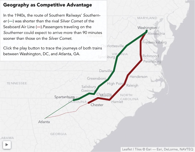
Figure 6-13. Maps built in the browser with a map library can use interactivity to build interest.
Summing Up
In this chapter, we’ve looked at several visualizations based on maps. In the first two examples, geographic regions were the main subjects of the visualization, and we built choropleth maps to compare and contrast those regions. Map fonts are quick and convenient, but only if they’re available for the regions the visualization needs. Although it usually takes more effort, we have far more control over the map regions if we use SVGs to create our own custom maps. Unlike other image formats, SVG can be easily manipulated in a web page with just CSS and JavaScript. This chapter also looked at examples based on traditional mapping libraries. Mapping libraries are especially convenient when your data sets include latitude and longitude values, as the libraries take care of the complicated mathematics required to position those points on a two-dimensional projection. As we saw, some libraries are relatively simple yet perfectly capable of mapping a data set. Full-featured libraries such as Leaflet offer much more power and customization, and we relied on that extensibility for a custom, animated map.
All materials on the site are licensed Creative Commons Attribution-Sharealike 3.0 Unported CC BY-SA 3.0 & GNU Free Documentation License (GFDL)
If you are the copyright holder of any material contained on our site and intend to remove it, please contact our site administrator for approval.
© 2016-2025 All site design rights belong to S.Y.A.