Excel 2016 All-in-One For Dummies (2016)

Book II

Worksheet Design

Chapter 5

Printing Worksheets

In This Chapter

Previewing pages and printing from the Excel Backstage view

Quick Printing from the Quick Access toolbar

Printing all the worksheets in a workbook

Printing just some of the cells in a worksheet

Changing page orientation

Printing the whole worksheet on a single page

Changing margins for a report

Adding a header and footer to a report

Printing column and row headings as print titles on every page

Inserting page breaks in a report

Printing the formulas in your worksheet

Printing the spreadsheet is one of the most important tasks that you do in Excel (second only to saving your spreadsheet in the first place). Fortunately, Excel makes it easy to produce professional-looking reports from your worksheets. This chapter covers how to select the printer that you want to use; print all or just selected parts of the worksheet; change your page layout and print settings, including the orientation, paper size, print quality, number of copies, and range of pages, all from the Excel 2016 Backstage view. The chapter also enlightens you on how to use the Ribbon to set up reports using the correct margin settings, headers and footers, titles, and page breaks and use the Page Layout, Print Preview, and Page Break Preview features to make sure that the pages of your report are the way you want them to appear before you print them.

The printing techniques covered in this chapter focus primarily on printing the data in your spreadsheets. Of course, in Excel you can also print your charts in chart sheets. Not surprisingly, you will find that most of the printing techniques that you learn for printing worksheet data in this chapter also apply to printing charts in their respective sheets. (For specific information on printing charts, see Book V, Chapter 1.)

Printing from the Excel 2016 Backstage View

The Excel 2016 Backstage view contains a Print screen (shown in Figure 5-1) opened by choosing File  ⇒  Print or pressing Ctrl+P. This Print screen enables you to do any of the following:

· Change the number of spreadsheet report copies to be printed (1 copy is the default) by entering a new value in the Copies combo box.

· Select a new printer to use in printing the spreadsheet report from the Printer drop-down list box. (See “Selecting the printer to use” that follows for details.)

· Change what part of the spreadsheet is printed in the report by selecting a new preset in the Active Sheets button’s drop-down menu — you can choose between Print Active Sheets (the default), Print Entire Workbook, or Print Selection — or by entering a new value in the Pages combo boxes immediately below. Select the Ignore Print Area at the bottom of the Active Sheets button’s drop-down menu when you want one of the other Print What options (Active Sheets, Entire Workbook, or Selection) that you selected to be used in the printing rather than the Print Area you previously defined. (See the “Setting and clearing the Print Area” section later in this chapter for details on how to set this area.)

· Print on both sides of the paper (assuming that your printer is capable of double-sided printing) by choosing either the Print on Both Sides, Flip Pages on Long Edge, or the Print on Both Sides, Flip Pages on Short Edge option from the Print One-Sided button’s drop-down menu.

· Print multiple copies of the spreadsheet report without having your printer collate the pages of each copy (collating the copies is the default) by choosing the Uncollated option from the Collated button’s drop-down menu.

· Change the orientation of the printing on the paper from the default portrait orientation to landscape (so that more columns of data and fewer rows are printed on each page of the report) by choosing the Landscape Orientation option from the Page Orientation button’s drop-down menu.

· Change the paper size from Letter (8.5 x 11 in) to another paper size supported by your printer by choosing its option from the Page Size button’s drop-down menu.

· Change the margins from the default Normal margins to Wide, Narrow, or the Last Custom Setting (representing the margin settings you last manually set for the report) by choosing these presets from the Margins button’s drop-down menu. (See “Massaging the margins” later in this chapter for details.)

· Scale the worksheet so that all its columns or all its rows or all of its columns and rows fit onto a single printed page.

· Change the default settings used by your printer by using the options in the particular printer’s Options dialog box. (These settings can include the print quality and color versus black and white or grayscale, depending upon the type of printer.) Open it by clicking the Printer Properties link right under the name of your printer in the Print screen.

· Preview the pages of the spreadsheet report on the right side of the Print screen. (See “Previewing the printout” later in this chapter for details.)

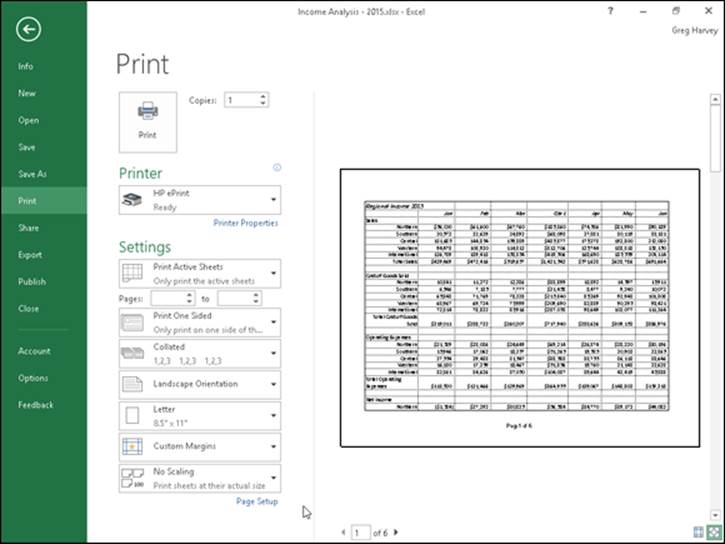
Figure 5-1: Previewing your printout report and changing common print settings is a snap using the Print screen in the Excel 2016 Backstage view.

Selecting the printer to use

Windows allows you to install more than one printer for use with your applications. If you’ve installed multiple printers, the first one installed becomes the default printer, which is used by all Windows applications, including Excel 2016. If you get a new printer, you must first install it from the Windows Control Panel before you can select and use the printer in Excel.

To select a new printer to use in printing the current worksheet, follow these steps:

1. Open the workbook with the worksheet that you want to print, activate that worksheet, and then choose File  ⇒  Print or simply press Ctrl+P.

The Print screen opens in the Backstage view (similar to the one shown in Figure 5-1). Be sure that you don’t click the Quick Print button if you’ve added it to the Quick Access toolbar (as described later in this chapter), because doing so sends the active worksheet directly to the default printer (without giving you an opportunity to change the printer!).

2. Select the name of the new printer that you want to use from the Printer drop-down list box.

If the printer that you want to use isn’t listed in the drop-down list, you can try to add the printer with the Add Printer link near the bottom of the list. When you click this button, Excel opens the Find Printers dialog box, where you specify the location for the program to search for the printer that you want to use. Note that if you don’t have a printer connected to your computer, clicking the Find Printer button and opening the Find Printers dialog box results in opening a Find in the Directory alert dialog box with the message, “The Active Directory Domain Services is Currently Unavailable.” When you click OK in this alert dialog box, Excel closes it as well as the Find Printers dialog box.

3. To change any of the default settings for the printer that you’ve selected, click the Printer Properties link Print and then select the new settings in the Properties dialog box for the printer that you selected.

4. Make any other required changes using the options (Pages, Collated, and so on) in the Settings section of the Print screen.

5. Click the Print button near the top of the left side of the Print screen to print the specified worksheet data using the newly selected printer.

Keep in mind that the printer you select and use in printing the current worksheet remains the selected printer in Excel until you change back to the original printer (or some other printer).

Previewing the printout

Excel 2016 gives you two ways to check the page layout before you send the report to the printer. In the worksheet, you can use the Page Layout view in the regular worksheet window that shows all the pages plus the margins along with the worksheet and row headings and rulers. Or, in the Excel Backstage view, you can use the old standby Print Preview on the right side of the Print screen, which shows you the pages of the report more or less as they appear on the printed page.

Checking the paging in Page Layout view

The Page Layout view — activated by clicking the Page Layout View button (the center one) to the immediate left of the Zoom slider on the status bar or the Page Layout View command button on the View tab of the Ribbon — gives you instant access to the paging of the active worksheet.

As you can see in Figure 5-2, when you switch to Page Layout view, Excel adds horizontal and vertical rulers to the column letter and row number headings. In the Worksheet area, this view shows the margins for each printed page with any headers and footers defined for the report along with the breaks between each. (Often you have to use the Zoom slider to reduce the screen magnification to display the page breaks on the screen.)

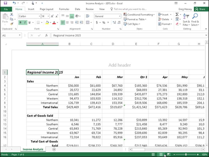
Figure 5-2: Viewing a spreadsheet in Page Layout view.

To see all the pages required to print the active worksheet, drag the slider button in the Zoom slider on the status bar to the left until you decrease the screen magnification sufficiently to display all the pages of data.

Excel displays rulers using the default units for your computer (inches on a United States computer and centimeters on a European machine). To change the units, open the Advanced tab of the Excel Options dialog box (File  ⇒  Options  ⇒  Advanced or Alt+FTA) and then choose the appropriate unit from the Ruler Units drop-down menu (Inches, Centimeters, or Millimeters) in the Display section. Remember that you can turn the rulers off and back on in Page Layout view by deselecting the Ruler check box in the Show group on the View tab (Alt+WR) and then selecting it again (Alt+WR).

Previewing the pages of the report

Stop wasting paper and save your sanity by using the Print Preview feature before you print any worksheet, section of a worksheet, or entire workbook. Because of the peculiarities in paging worksheet data, check the page breaks for any report that requires more than one page. You can use Print Preview in the Print screen of the Excel Backstage view to see exactly how the worksheet data will be paged when printed. That way, you can return to the worksheet and make any necessary last-minute changes to the data or page settings before sending the report on to the printer.

To switch to the Print screen and preview the printout, choose File  ⇒  Print or simply press Ctrl+P. Excel displays the first page of the report on the right side of the Print screen. Look at Figure 5-3 to see the first preview page of a ten-page report as it initially appears in the Print screen.

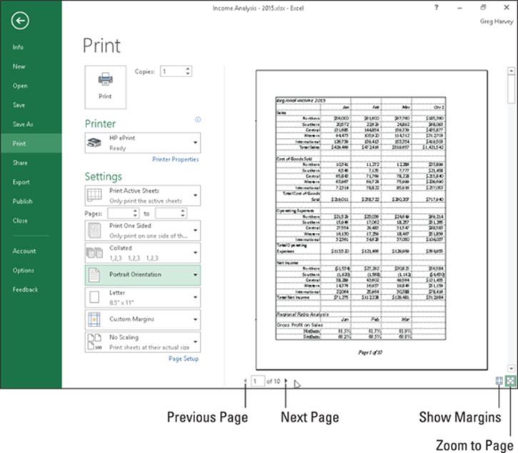
Figure 5-3: Page 1 of a ten-page report in Print Preview.

If you use Print Preview frequently (as you should), you might want to add the Print Preview button to the Quick Access toolbar and then open the Print screen in the Backstage view by clicking this button. To add a Print Preview button, click the Customize Quick Access Toolbar button and then choose the Print Preview option under Quick Print from its drop-down menu. (To remove the button, simply choose this same Print Preview option from the Customize Quick Access drop-down menu a second time.)

When Excel displays a full page in the Print Preview window, you sometimes can barely read its contents. In such a case, you can increase the view to actual size when you need to verify specific regions of the worksheet by clicking the Zoom to Page button at the bottom of the Print screen. Check out the difference in Figure 5-4 — here you can see what the first page of the ten-page report looks like after I zoom in by clicking the Zoom to Page button.

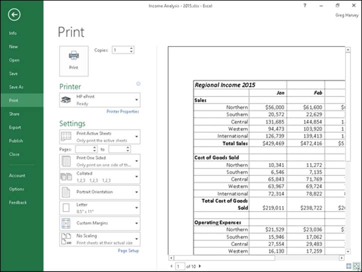
Figure 5-4: Page 1 of a ten-page report after selecting the Zoom to Page button at the bottom of the Print screen.

After you enlarge a page to actual size, use the scroll bars to bring new parts of the page into view in the Print Preview window. To return to the full-page view, you simply deselect the Zoom to Page button by clicking it a second time.

Excel indicates the number of pages in a report at the bottom left of the Print Preview area. If your report has more than one page, view pages that follow by clicking the Next Page button. To review a page you’ve already seen, back up a page by clicking the Previous Page button immediately below it. (The Previous Page button is grayed out if you’re on the first page.) You can also advance to a particular page in the report by typing its page number into the text box to the immediate right of the Previous Page button that shows the current page and then pressing the Enter key.

If you want to display the current margin settings for the report in the print preview area, click the Show Margins button at the bottom of the Print screen to the immediate left of the Zoom to Page button. After the margins are displayed, you can then manually manipulate them by dragging them to new positions. (See “Massaging the margins” later in this chapter for details.)

When you finish previewing the report, you can print the spreadsheet report by clicking the Print button in the Print screen or you can exit the Backstage view and return to the worksheet by clicking the Back button at the very top of the File menu along the left side of the screen.

Quick Printing the Worksheet

As long as you want to use Excel’s default print settings to print all the cells in the current worksheet, printing in Excel 2016 is a breeze. Simply add the Quick Print button to the Quick Access toolbar by clicking the Customize Quick Access Toolbar button and then choosing the Quick Print item from its drop-down menu.

After adding the Quick Print button to the Quick Access toolbar, you can use this button to print a single copy of all the information in the current worksheet, including any charts and graphics, everything but the comments you’ve added to cells.

When you click the Quick Print button, Excel routes the print job to the Windows print queue, which acts like a middleman and sends the job to the printer. While Excel sends the print job to the print queue, Excel displays a Printing dialog box to inform you of its progress (displaying such updates as Printing Page 2 of 3). After this dialog box disappears, you are free to go back to work in Excel. To stop the printing while the job is still being sent to the print queue, click the Cancel button in the Printing dialog box.

If you don’t realize that you want to cancel the print job until after Excel finishes shipping it to the print queue (that is, while the Printing dialog box appears onscreen), you must take these steps:

1. Right-click the printer icon in the notification area at the far right of the Windows taskbar and then select the Open All Active Printers command from its shortcut menu.

This opens the dialog box for the printer with the Excel print job in its queue (as described under the Document Name heading in the list box).

2. Select the Excel print job that you want to cancel in the list box of your printer’s dialog box.

3. Choose Document  ⇒  Cancel from the menu bar and then click Yes to confirm you want to cancel the print job.

4. Wait for the print job to disappear from the queue in the printer’s dialog box and then click the Close button to return to Excel.

Working with the Page Setup Options

About the only thing the slightest bit complex in printing a worksheet is figuring out how to get the pages right. Fortunately, the command buttons in the Page Setup group on the Ribbon’s Page Layout tab give you a great deal of control over what goes on which page.

There are three groups of buttons on the Page Layout tab that are helpful in getting your page settings exactly as you want them: the Page Setup group, the Scale to Fit group, and the Sheet Options group, all described in upcoming sections.

To see the effect of changes you make to the page setup settings in the Worksheet area, put the worksheet into Page Layout view by clicking the Page Layout button on the status bar as you work with the command buttons in Page Setup, Scale to Fit, and Sheet Options groups on the Page Layout tab.

Using the buttons in the Page Setup group

The Page Setup group of the Page Layout tab contains the following important command buttons:

· Margins: Select one of three preset margins for the report or to set custom margins on the Margins tab of the Page Setup dialog box. (See “Massaging the margins” later in this chapter.)

· Orientation: Choose between Portrait and Landscape mode for the printing. (See “Getting the lay of the landscape” later in this chapter.)

· Size: Select one of the preset paper sizes or to set a custom size or to change the printing resolution or page number on the Page tab of the Page Layout dialog box.

· Print Area: Set and clear the Print Area. (See “Setting and clearing the Print Area” immediately following in this chapter.)

· Breaks: Insert or remove page breaks. (See “Solving Page Break Problems” later in this chapter.)

· Background: Open the Sheet Background dialog box, where you can select a new graphic image or photo to be used as a background for all the worksheets in the workbook. (Note that this button changes to Delete Background as soon as you select a background image.)

· Print Titles: Open the Sheet tab of the Page Setup dialog box, where you can define rows of the worksheet to repeat at the top and columns at the left as print titles for the report. (See “Putting out the print titles” later in this chapter.)

Setting and clearing the Print Area

Excel includes a special printing feature called the Print Area. You choose Print Area  ⇒  Set Print Area on the Ribbon’s Page Layout tab or press Alt+PRS to define any cell selection on a worksheet as the Print Area. After you define the Print Area, Excel then prints this cell selection anytime you print the worksheet (either with the Quick Print button on the Quick Access toolbar or by choosing File  ⇒  Print and then clicking the Print button on the Print screen).

Whenever you fool with the Print Area, you need to keep in mind that after you define it, its cell range is the only one you can print (regardless of what other print area options you select in the Print screen unless you click the Ignore Print Areas check box at the bottom of the very first drop-down menu in the Settings section of the Print screen and until you clear the Print Area).

To clear the Print Area (and therefore go back to the printing defaults Excel establishes in the Print screen), you just have to choose Print Area  ⇒  Clear Print Area on the Page Layout tab or simply press Alt+PRC.

Keep in mind that you can also define and clear the Print Area from the Sheet tab of the Page Setup dialog box opened by clicking the dialog box launcher button in the Page Setup group on the Page Layout Ribbon tab (Alt+PSP). To define the Print Area from this dialog box, click the Print Area text box on the Sheet tab to insert the cursor and then select the cell range or ranges in the worksheet. (Remember that you can reduce the Page Setup dialog box to just this text box by clicking its minimize box.) To clear the Print Area from this dialog box, select the cell addresses in the Print Area text box and press the Delete key.

Massaging the margins

The Normal margin settings that Excel applies to a new report use standard top and bottom margins of 0.75 inch (¾ inch) and left and right margins of 0.7 inch with just over a ¼ inch separating the header and footer from the top and bottom margins, respectively.

In addition to the Normal margin settings, the program enables you to choose two other standard margins from the Margins button’s drop-down menu in the Print screen (Ctrl+P):

· Wide margins with 1-inch top, bottom, left, and right margins and ½ inch separating the header and footer from the top and bottom margins, respectively.

· Narrow margins with top and bottom margins of ¾ inch, and left and right margins of ¼ inch with slightly more than ¼ inch separating the header and footer from the top and bottom margins, respectively.

Frequently, you find yourself with a report that takes up a full printed page and then just enough to spill over onto a second, mostly empty, page. To squeeze the last column or the last few rows of the worksheet data onto Page 1, try choosing Narrow from the Margins button’s drop-down menu.

If that doesn’t do it, you can try manually adjusting the margins for the report either from the Margins tab of the Page Setup dialog box or by dragging the margin markers in the print preview area on the Print screen in the Excel Backstage view. To get more columns on a page, try reducing the left and right margins. To get more rows on a page, try reducing the top and bottom margins.

To open the Margins tab of the Page Setup dialog box (shown in Figure 5-5), open the Page Setup dialog box (Alt+PSP) and then click the Margins tab. There, enter the new settings in the Top, Bottom, Left, and Right text boxes — or select the new margin settings with their respective spinner buttons.

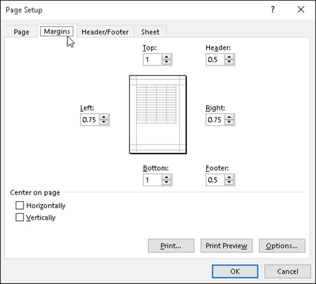
Figure 5-5: Adjust your report margins from the Margins tab in the Page Setup dialog box.

Select one or both Center on Page options in the Margins tab of the Page Setup dialog box (refer to Figure 5-5) to center a selection of data (that takes up less than a full page) between the current margin settings. In the Center on Page section, select the Horizontally check box to center the data between the left and right margins. Select the Vertically check box to center the data between the top and bottom margins.

If you select the Show Margins check box at the bottom of the Print screen in the Excel Backstage view (Ctrl+P) to change the margin settings, you can modify the column widths as well as the margins. (See Figure 5-6.) To change one of the margins, position the mouse pointer on the desired margin marker (the pointer shape changes to a double-headed arrow) and drag the marker with your mouse in the appropriate direction. When you release the mouse button, Excel redraws the page, using the new margin setting. You may gain or lose columns or rows, depending on what kind of adjustment you make. Changing the column width is the same story: Drag the column marker to the left or right to decrease or increase the width of a particular column.

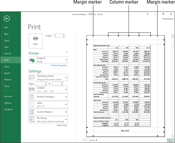
Figure 5-6: Drag a marker to adjust its margin in the Page Preview window when the Show Margins check box is selected.

Getting the lay of the landscape

The drop-down menu attached to the Orientation button in the Page Setup group of the Page Layout tab of the Ribbon contains two options:

· Portrait (the default), where the printing runs parallel to the short edge of the paper

· Landscape, where the printing runs parallel to the long edge of the paper

Because many worksheets are far wider than they are tall (such as budgets or sales tables that track expenditures across all 12 months), you may find that their worksheets page better if you switch the orientation from the normal portrait mode (which accommodates fewer columns on a page because the printing runs parallel to the short edge of the page) to landscape mode.

In Figure 5-7, you can see the Print screen in the Backstage view with the first page of a report in landscape mode in the Page Layout view. For this report, Excel can fit three more columns of information on this page in landscape mode than it can in portrait mode. Therefore, the total page count for this report decreases from ten pages in portrait mode to six pages in landscape mode.

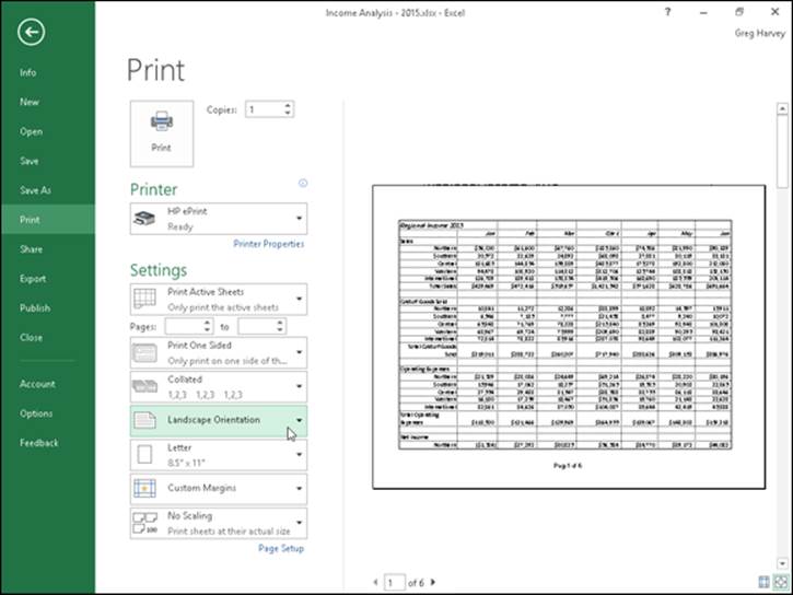
Figure 5-7: A landscape mode report in Page Layout view.

Putting out the print titles

Excel’s Print Titles enable you to print particular row and column headings on each page of the report. Print titles are important in multi-page reports where the columns and rows of related data spill over to other pages that no longer show the row and column headings on the first page.

Don’t confuse print titles with the header of a report. Even though both are printed on each page, header information prints in the top margin of the report; print titles always appear in the body of the report — at the top, in the case of rows used as print titles, and on the left, in the case of columns.

To designate rows and/or columns as the print titles for a report, follow these steps:

1. Click the Print Titles button on the Ribbon’s Page Layout tab or press Alt+PI.

The Page Setup dialog box appears with the Sheet tab selected (similar to the one shown in Figure 5-8).

To designate worksheet rows as print titles, go to Step 2a. To designate worksheet columns as print titles, go to Step 2b.

2a. Select the Rows to Repeat at Top text box and then drag through the rows with information you want to appear at the top of each page in the worksheet below. If necessary, reduce the Page Setup dialog box to just the Rows to Repeat at Top text box by clicking the text box’s Collapse/Expand button.

In the example I show you in Figure 5-8, I clicked the minimize button associated with the Rows to Repeat at Top text box and then dragged through rows 1 and 2 in column A of the Income Analysis worksheet, and the program entered the row range $1:$2 in the Rows to Repeat at Top text box.

Note that Excel indicates the print-title rows in the worksheet by placing a dotted line (that moves like a marquee) on the border between the titles and the information in the body of the report.

2b. Select the Columns to Repeat at Left text box and then drag through the range of columns with the information you want to appear at the left edge of each page of the printed report in the worksheet below. If necessary, reduce the Page Setup dialog box to just the Columns to Repeat at Left text box by clicking its Collapse/Expand button.

Note that Excel indicates the print-title columns in the worksheet by placing a dotted line (that moves like a marquee) on the border between the titles and the information in the body of the report.

3. Click OK or press Enter to close the Page Setup dialog box or click the Print Preview button to preview the page titles in the Print Preview pane on the Print screen.

After you close the Page Setup dialog box, the dotted line showing the border of the row and/or column titles disappears from the worksheet.

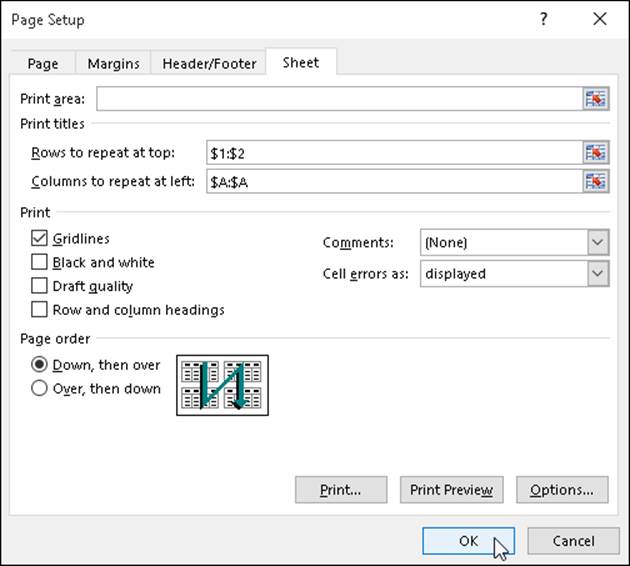
Figure 5-8: Specify the rows and columns to use as print titles on the Sheet tab of the Page Setup dialog box.

In Figure 5-8, rows 1 and 2 containing the worksheet title and column headings for the Income Analysis worksheet are designated as the print titles for the report. In Figure 5-9, you can see the Print Preview window with the second page of the report. Note how these print titles appear on all pages of the report.

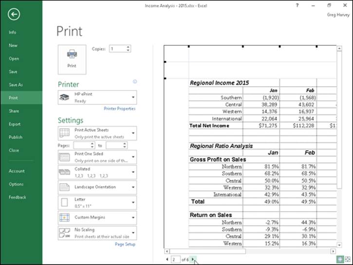
Figure 5-9: Page 2 of a sample report in Print Preview with defined print titles.

To clear print titles from a report if you no longer need them, open the Sheet tab of the Page Setup dialog box and then delete the row and column ranges from the Rows to Repeat at Top and the Columns to Repeat at Left text boxes before you click OK or press Enter.

Using the buttons in the Scale to Fit group

If your printer supports scaling options, you’re in luck. You can always get a worksheet to fit on a single page simply by selecting the 1 Page option on the Width and Height drop-down menus attached to their command buttons in the Scale to Fit group on the Layout Page tab of the Ribbon. When you select these options, Excel figures out how much to reduce the size of the information you’re printing to fit it all on one page.

If you preview this one page in the Print screen of the Backstage view (Ctrl+P) and find that the printing is just too small to read comfortably, return to the worksheet view. Then, reopen the Page tab of the Page Setup dialog box and try changing the number of pages in the Page(s) Wide and Tall text boxes (to the immediate right of the Fit To option button).

Instead of trying to stuff everything on one page, check out how your worksheet looks if you fit it on two pages across. Try this: Select 2 Pages from the Width button’s drop-down list on the Page Layout tab and leave 1 Page selected in the Height drop-down list. Alternatively, see how the worksheet looks on two pages down: Select 1 Page from the Width button’s drop-down list and 2 Pages from the Height button’s drop-down list.

After using the Width and Height Scale to Fit options, you may find that you don’t want to scale the printing. Cancel scaling by selecting Automatic on both the Width and Height drop-down lists and then entering 100 in the Scale text (or select 100 with its spinner buttons).

Using the Print buttons in the Sheet Options group

The Sheet Options group on the Ribbon’s Page Layout tab contains two very useful Print check boxes (neither of which is automatically selected). The first is in the Gridlines column and the second in the Headings column:

· Select the Print check box in the Gridlines column to print the column and row gridlines on each page of the report.

· Select the Print check box in the Headings column to print the row headings with the row numbers, and the column headings with the column letters on each page of the report.

Select both check boxes (by clicking them to put check marks in them) when you want the printed version of your spreadsheet data to match as closely as possible their onscreen appearance. This is useful when you need to use the cell references on the printout to help you later locate the cells in the actual worksheet that needs editing.

Headers and Footers

Headers and footers are simply standard text that appears on every page of the report. A header is printed in the top margin of the page, and a footer is printed — you guessed it — in the bottom margin. Both are centered vertically in the margins. Unless you specify otherwise, Excel does not automatically add either a header or footer to a new workbook.

Use headers and footers in a report to identify the document used to produce the report and display the page numbers and the date and time of printing.

The easiest way to add a header or footer to a report is to add it after putting the worksheet in Page Layout view by clicking the Page Layout View button on the status bar (or by clicking the Page Layout View button on the Ribbon’s View tab or by just pressing Alt+WP).

When the worksheet is displayed in Page Layout view, position the mouse pointer over the section in the top margin of the first page marked Add Header or in the bottom margin of the first page marked Add Footer.

To create a centered header or footer, highlight the center section of this header/footer area and then click the mouse pointer to set the insertion point in the middle of the section. To add a left-aligned header or footer, highlight and then click to set the insertion point flush with the left edge of the left section, or to add a right-aligned header or footer, highlight and click to set the insertion point flush with the right edge of the right section.

Immediately after setting the insertion point in the left, center, or right section of the header/footer area, Excel adds a Header & Footer Tools contextual tab with its own Design tab. (See Figure 5-10.) The Design tab is divided into Header & Footer, Header & Footer Elements, Navigation, and Options groups.

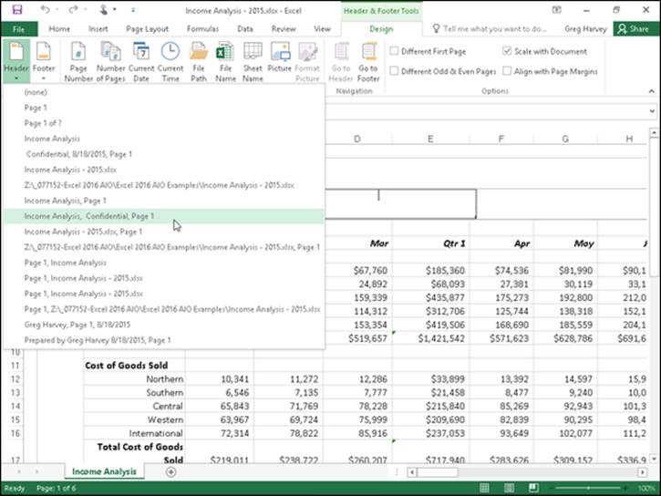
Figure 5-10: Defining a new header using the Header drop-down menu on the Design tab of the Header & Footer Tools contextual tab.

Adding a ready-made header or footer

The Header and Auto Footer buttons on the Design tab of the Header & Footer Tools contextual tab enable you to add stock headers and footers in an instant simply by clicking their examples from the drop-down menus that appear when you click them.

To create the centered header and footer for the report shown in Figure 5-11, I first chose

Income Analysis, Confidential, Page 1

from the Header button’s drop-down menu. (Income Analysis is the name of the worksheet; Confidential is stock text; and Page 1 is, of course, the current page number.)

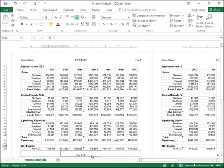
Figure 5-11: The first page of a report in Page Layout view shows you how the header and footer will print.

To set up the footer, I chose

Page 1 of ?

from the Footer button’s drop-down menu (which puts the current page number, along with the total number of pages, in the report). You can choose this paging option from either the Header or Footer drop-down menu.

Check out the results in Figure 5-11, which is the first page of the report in Page Layout view. Here you can see the header and footer as they will print. You can also see how choosing Page 1 of ? works in the footer: On the first page, you see the centered footer: Page 1 of 6; on the second page, you would see the centered footer Page 2 of 6.

If, after selecting a ready-made header or footer, you decide that you no longer need either the header or footer printed in your report, click the header or footer in Page Layout view and then choose the (none) option at the top of the Header button’s or Footer button’s drop-down menu. (The Design tab on the Header & Footer Tools contextual tab automatically appears and is selected on the Ribbon the moment you click the header or footer in Page Layout view.)

Creating a custom header or footer

Most of the time, the stock headers and footers available on the Header button’s and Footer button’s drop-down menus are sufficient for your report printing needs. Every once in a while, however, you may want to insert information not available in these list boxes or in an arrangement Excel doesn’t offer in the ready-made headers and footers.

For those times, you need to use the command buttons that appear in the Header & Footer Elements group of the Design tab on the Header & Footer Tools contextual tab. These command buttons enable you to blend your own information with that generated by Excel into different sections of the custom header or footer you’re creating.

The command buttons in the Header & Footer Elements group include the following:

· Page Number: Click this button to insert the &[Page] code that puts in the current page number.

· Number of Pages: Click this button to insert the &[Pages] code that puts in the total number of pages.

· Current Date: Click this button to insert the &[Date] code that puts in the current date.

· Current Time: Click this button to insert the &[Time] code that puts in the current time.

· File Path: Click this button to insert the &[Path]&[File] code that puts in the directory path along with the name of the workbook file.

· File Name: Click this button to insert the &[File] code that puts in the name of the workbook file.

· Sheet Name: Click this button to insert the &[Tab] code that puts in the name of the worksheet as shown on the sheet tab.

· Picture: Click this button to insert the &[Picture] code that inserts the image that you select from the Insert Pictures dialog box that enables you to get a graphics file on your computer or download one (see Book V, Chapter 2 for more on inserting pictures).

· Format Picture: Click this button to apply the formatting that you choose from the Format Picture dialog box to the &[Picture] code that you enter with the Insert Picture button without adding any code of its own.

To use these command buttons in the Header & Footer Elements group to create a custom header or footer, follow these steps:

1. Put your worksheet into Page Layout view by clicking the Page Layout View button on the status bar, or by choosing View  ⇒  Page Layout View on the Ribbon, or by pressing Alt+WP.

In Page Layout view, the text Add Header appears centered in the top margin of the first page, and the text Add Footer appears centered in the bottom margin.

2. Position the mouse or Touch pointer in the top margin to create a custom header or in the bottom margin to create a custom footer, and then click the pointer in the left, center, or right section of the header or footer to set the insertion point and left-align, center, or right-align the text.

When Excel sets the insertion point, the text, Add Header and Add Footer, disappears, and the Design tab on the Header & Footer Tools contextual tab becomes active on the Ribbon.

3. To add program-generated information to your custom header or footer such as the filename, worksheet name, current date, and so forth, click its command button in the Header & Footer Elements group.

Excel inserts the appropriate header/footer code preceded by an ampersand (&) in the header or footer. These codes are replaced by the actual information (filename, worksheet name, graphic image, and the like) as soon as you click another section of the header or footer or finish the header or footer by clicking the mouse pointer outside of it.

4. (Optional) To add your own text to the custom header or footer, type it at the insertion point.

When joining program-generated information indicated by a header/footer code with your own text, be sure to insert the appropriate spaces and punctuation. For example, to have Excel display Page 1 of 4 in a custom header or footer, you do the following:

1. Type the word Page and press the spacebar.

2. Click the Page Number command button and press the spacebar again.

3. Type the word of and press the spacebar a third time.

4. Click the Number of Pages command button.

This inserts Page &[Page] of &[Pages] in the custom header (or footer).

5. (Optional) To modify the font, font size, or some other font attribute of your custom header or footer, drag through its codes and text, click the Home tab, and then click the appropriate command button in the Font group.

In addition to selecting a new font and font size for the custom header or footer, you can add bold, italics, underlining, and a new font color to its text with the Bold, Italic, Underline, and Font Color command buttons on the Home tab.

6. After you finish defining and formatting the codes and text in your custom header or footer, click a cell in the Worksheet area to deselect the header or footer area.

Excel replaces the header/footer codes in the custom header or footer with the actual information, while at the same time removing the Header & Footer Tools contextual tab from the Ribbon.

Figure 5-12 shows you a custom footer I added to a spreadsheet in Page Layout view. This custom footer blends my own text with program-generated page, date, and time information, and uses all three sections: left-aligned page information, a centered Preliminary warning, and right-aligned current date and time.

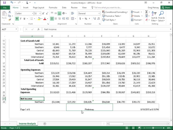
Figure 5-12: A spreadsheet in Page Layout view showing the custom footer.

Creating unique first-page headers and footers

Excel 2016 enables you to define a header or footer for the first page that’s different from all the rest of the pages. Simply click the Different First Page check box to put a check mark in it. (This check box is part of the Options group of the Design tab on the Header & Footer Tools contextual tab that appears when you’re defining or editing a header or footer in Page Layout view.)

After selecting the Different First Page check box, go ahead and define the unique header and/or footer for just the first page (now marked First Page Header or First Page Footer). Then, on the second page of the report, define the header and/or footer (marked simply Header or Footer) for the remaining pages of the report. (See “Adding a ready-made header or footer” and “Creating a custom header or footer” earlier in the chapter for details.)

Use this feature when your spreadsheet report has a cover page that needs no header or footer. For example, say you have a report that needs the current page number and total pages centered at the bottom of all pages but the first, cover page. To do this, select the Different First Page check box on the Design tab of the Header & Footer Tools contextual tab on the Ribbon and then define a centered stock footer that displays the current page number and total pages (Page 1 of ?) on the second page of the report, leaving the Add Footer text intact on the first page.

Excel correctly numbers both the total number of pages in the report and the current page number without printing this information on the first page. So if your report has a total of six pages (including the cover page), the second page footer will read Page 2 of 6; the third page, Page 3 of 6; and so on, even if the first printed page has no footer at all.

Creating different even and odd page headers and footers

If you plan to do two-sided printing or copying of your spreadsheet report, you may want to define one header or footer for the even pages and another for the odd pages of the report. That way, the header or footer information (such as the report name or current page) alternates from being right-aligned on the odd pages (printed on the front side of the page) to being left-aligned on the even pages (printed on the back side of the page).

To create an alternating header or footer for a report, you click the Different Odd & Even Pages check box to put a check mark in it. (This check box is found in the Options group of the Design tab on the Header & Footer Tools contextual tab that appears when you’re defining or editing a header or footer in Page Layout view.)

After that, create a header or footer on the first page of the report (now marked Odd Page Header or Odd Page Footer) in the third, right-aligned section header or footer area and then re-create this header or footer on the second page (now marked Even Page Header or Even Page Footer), this time in the first, left-aligned section.

Solving Page Break Problems

The Page Break Preview feature in Excel enables you to spot page break problems in an instant as well as fix them, such as when the program wants to split onto different pages information that you know should always appear on the same page.

Figure 5-13 shows a worksheet in Page Break Preview with an example of a bad vertical and horizontal page break that you can remedy by adjusting the location of the page break on Pages 1 and 3. Given the page size, orientation, and margin settings for this report, Excel inserts a vertical page break between columns H and I. This break separates the April, May, and June sales on Page 1 from the Qtr 2 subtotals on Page 3. It also inserts a horizontal page break between rows 28 and 29, splitting the Net Income heading from its data in the rows below.

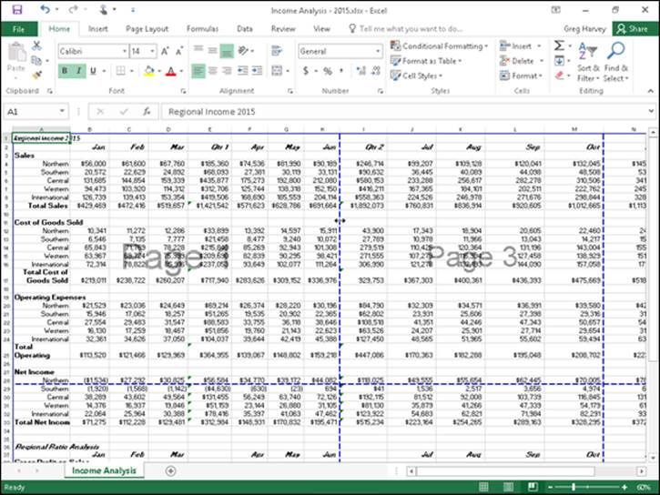
Figure 5-13: Preview page breaks in a report in Page Break Preview.

To correct the bad vertical page break, you need to move the page break to a column on the left several columns so that it occurs between columns E (with the Qtr 1 subtotals) and F (containing the April sales) so that the second quarter sales and subtotals are printed together on Page 3. To correct the bad horizontal page break, you need to move that break up one row so that the Net Income heading prints on the page with its data on Page 2.

Figure 5-13 illustrates how you can correct these two bad page breaks in Page Break Preview mode by following these steps:

1. Click the Page Break Preview button (the third one in the cluster of three to the left of the Zoom slider) on the status bar, or choose View  ⇒  Page Break Preview on the Ribbon, or press Alt+WI.

This takes you into a Page Break Preview mode that shows your worksheet data at a reduced magnification (60 percent of normal in Figure 5-13) with the page numbers displayed in large, light type and the page breaks shown by heavy lines between the columns and rows of the worksheet.

2. Position the mouse or Touch pointer somewhere on the page break indicator (one of the heavy lines surrounding the representation of the page) that you need to adjust; when the pointer changes to a double-headed arrow, drag the page indicator to the desired column or row and release the mouse button.

For the example shown in Figure 5-13, I dragged the page break indicator between Pages 1 and 3 to the left so that it’s between columns E and F and the page indicator between Page 1 and 2 up so that its between row 26 and 27.

In Figure 5-14, you can see Page 1 of the report as it then appears in the Print Preview window.

3. After you finish adjusting the page breaks in Page Break Preview (and, presumably, printing the report), click the Normal button (the first one in the cluster of three to the left of the Zoom slider) on the status bar, or choose View  ⇒  Normal on the Ribbon, or press Alt+WL to return the worksheet to its regular view of the data.

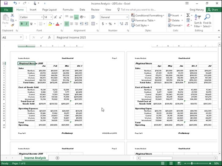
Figure 5-14: Page 1 of the report in the Print Preview window after adjusting the page breaks in Page Break Preview mode.

You can also insert your own manual page breaks at the cell cursor’s position by choosing Insert Page Break from the Breaks button’s drop-down menu on the Page Layout tab (Alt+PBI), and you can remove them by choosing Remove Page Break from this menu (Alt+PBR). To remove all manual page breaks that you’ve inserted into a report, choose Reset All Page Breaks from the Breaks button’s drop-down menu (Alt+PBA).

Printing the Formulas in a Report

There’s one more printing technique you may need every once in a while, and that’s how to print the formulas in a worksheet in a report instead of printing the calculated results of the formulas. You can check over a printout of the formulas in your worksheet to make sure that you haven’t done anything stupid (like replace a formula with a number or use the wrong cell references in a formula) before you distribute the worksheet company wide.

Before you can print a worksheet’s formulas, you have to display the formulas, rather than their results, in the cells by clicking the Show Formulas button (the one that kind of looks like a page of a calendar with a tiny 15 above an fx) in the Formula Auditing group on the Formulas tab of the Ribbon (Alt+MH).

Excel then displays the contents of each cell in the worksheet as they normally appear only in the Formula bar or when you’re editing them in the cell. Notice that value entries lose their number formatting, formulas appear in their cells (Excel widens the columns with best-fit so that the formulas appear in their entirety), and long text entries no longer spill over into neighboring blank cells.

Excel allows you to toggle between the normal cell display and the formula cell display by pressing Ctrl+`. (That is, press Ctrl and the key with the tilde on top.) This key — usually found in the upper-left corner of your keyboard — does double-duty as a tilde and as a weird backward accent mark: ` (Don’t confuse that backward accent mark with the apostrophe that appears on the same key as the quotation mark!)

After Excel displays the formulas in the worksheet, you are ready to print it as you would any other report. You can include the worksheet column letters and row numbers as headings in the printout so that if you do spot an error, you can pinpoint the cell reference right away.

To include the row and column headings in the printout, put a check mark in the Print check box in the Headings column on the Sheet Options group of the Page Layout tab of the Ribbon before you send the report to the printer.

After you print the worksheet with the formulas, return the worksheet to normal by clicking the Show Formulas button on the Formulas tab of the Ribbon or by pressing Ctrl+’.