Excel 2016 All-in-One For Dummies (2016)

Book III

Formulas and Functions

Chapter 2

Logical Functions and Error Trapping

In This Chapter

Understanding formula error values

Understanding the logical functions

Creating IF formulas that trap errors

Auditing formulas

Changing the Error Checking options

Masking error values in your printouts

Troubleshooting the formula errors in a worksheet is the main topic of this chapter. Here, you see how to locate the source of all those vexing formula errors so that you can shoot them down and set things right! The biggest problem with errors in your formulas — besides how ugly such values as #REF! and #DIV/0! are — is that they spread like wildfire through the workbook to other cells containing formulas that refer to their error-laden cells. If you’re dealing with a large worksheet in a really big workbook, you may not be able to tell which cell actually contains the formula that’s causing all the hubbub. And if you can’t apprehend the cell that is the cause of all this unpleasantness, you really have no way of restoring law and order to your workbook.

Keeping in mind that the best defense is a good offense, you also find out in this chapter how to trap potential errors at their source and thereby keep them there. This technique, known affectionately as error trapping (just think of yourself as being on a spreadsheet safari), is easily accomplished by skillfully combining the IF function to combine with the workings of the original formula.

Understanding Error Values

If Excel can’t properly calculate a formula that you enter in a cell, the program displays an error value in the cell as soon as you complete the formula entry. Excel uses several error values, all of which begin with the number sign (#). Table 2-1 shows you the error values in Excel along with the meanings and the most probable causes for their display. To remove an error value from a cell, you must discover what caused the value to appear and then edit the formula so that Excel can complete the desired calculation.

Table 2-1 Error Values in Excel

If a formula in your worksheet contains a reference to a cell that returns an error value, that formula returns that error value as well. This can cause error values to appear throughout the worksheet, thus making it very difficult for you to discover which cell contains the formula that caused the original error value so that you can fix the problem.

Using Logical Functions

Excel uses the following logical functions, which appear on the Logical command button’s drop-down menu on the Formulas tab of the Ribbon (Alt+ML). All the logical functions return either the logical TRUE or logical FALSE to their cells when their functions are evaluated. Here are the names of the functions along with their argument syntax:

· AND(logical1,logical2,…) — tests whether the logical arguments are TRUE or FALSE. If they are all TRUE, the AND function returns TRUE to the cell. If any are FALSE, the AND function returns FALSE.

· FALSE( ) — takes no argument and simply enters logical FALSE in its cell.

· IF(logical_test,value_if_true,value_if_false) — tests whether the logical_test expression is TRUE or FALSE. If TRUE, the IF function uses the value_if_true argument and returns it to the cell. If FALSE, the IF function uses the value_if_false argument and returns it to the cell.

· IFERROR(value,value_if_error) — returns the value argument when the cell referred to in another logical argument in which the IFERROR function is used doesn’t contain an error value and the value_if_error argument when it does.

· IFNA(value,value_if_na) — returns the value argument when the cell referred to in another logical argument in which the IFNA function is used doesn’t contain #NA and the value_if_error argument when it does.

· NOT(logical) — tests whether the logical argument is TRUE or FALSE. If TRUE, the NOT function returns FALSE to the cell. IF FALSE, the NOT function returns TRUE to the cell.

· OR(logical1,logical2,…) — tests whether the logical arguments are TRUE or FALSE. If any are TRUE, the OR function returns TRUE. If all are FALSE, the OR function returns FALSE.

· TRUE( ) — takes no argument and simply enters logical TRUE in its cell.

· XOR(logical1,logical2,…) — tests whether the logical arguments (usually in an array) are predominantly TRUE or FALSE. When the number of TRUE inputs is odd, the XOR function returns TRUE. When the number of TRUE inputs is even, the XOR function returns FALSE.

The logical_test and logical arguments that you specify for these logical functions usually employ the comparison operators (=, <, >, <=, >=, or <>), which themselves return logical TRUE or logical FALSE values. For example, suppose that you enter the following formula in your worksheet:

=AND(B5=D10,C15>=500)

In this formula, Excel first evaluates the first logical argument to determine whether the contents in cell B5 and D10 are equal to each other. If they are, the first comparison returns TRUE. If they are not equal to each other, this comparison returns FALSE. The program then evaluates the second logical argument to determine whether the content of cell C15 is greater than or equal to 500. If it is, the second comparison returns TRUE. If it is not greater than or equal to 500, this comparison returns FALSE.

After evaluating the comparisons in the two logical arguments, the AND function compares the results: If logical argument 1 and logical argument 2 are both found to be TRUE, the AND function returns logical TRUE to the cell. If, however, either argument is found to be FALSE, the AND function returns FALSE to the cell.

When you use the IF function, you specify what’s called a logical_test argument whose outcome determines whether the value_if_true or value_if_false argument is evaluated and returned to the cell. The logical_test argument normally uses comparison operators, which return either the logical TRUE or logical FALSE value. When the argument returns TRUE, the entry or expression in the value_if_true argument is used and returned to the cell. When the argument returns FALSE, the entry or expression in the value_if_false argument is used.

Consider the following formula that uses the IF function to determine whether to charge tax on an item:

=IF(E5="Yes",D5+D5*7.5%,D5)

If cell E5 (the first cell in the column where you indicate whether the item being sold is taxable or not) contains “Yes,” the IF function uses the value_if_true argument that tells Excel to add the extended price entered in cell D5, multiply it by a tax rate of 7.5%, and then add the computed tax to the extended price. If, however, cell D5 is blank or contains anything other than the text “Yes,” the IF function uses the value_if_false argument, which tells Excel to just return the extended price to cell D5 without adding any tax to it.

As you can see, the value_if_true and value_if_false arguments of the IF function can contain constants or expressions whose results are returned to the cell that holds the IF formula.

Error-Trapping Formulas

Sometimes, you know ahead of time that certain error values are unavoidable in a worksheet as long as it’s missing certain data. The most common error value that gets you into this kind of trouble is our old friend, the #DIV/0! error value. Suppose, for example, that you’re creating a new sales workbook from your sales template, and one of the rows in this template contains formulas that calculate the percentage that each monthly total is of the quarterly total. To work correctly, the formulas must divide the value in the cell that contains the monthly total by the value in the cell that contains the quarterly total. When you start a new sales workbook from its template, the cells that contain the formulas for determining the quarterly totals contain zeros, and these zeros put #DIV/0! errors in the cells with formulas that calculate the monthly/quarterly percentages.

These particular #DIV/0! error values in the new workbook don’t really represent mistakes as such because they automatically disappear as soon as you enter some of the monthly sales for each quarter (so that the calculated quarterly totals are no longer 0). The problem that you may have is convincing your non-spreadsheet-savvy co-workers (especially the boss) that, despite the presence of all these error values in your worksheet, the formulas are hunky-dory. All that your co-workers see is a worksheet riddled with error values, and these error values undermine your co-workers’ confidence in the correctness of your worksheet.

Well, I have the answer for just such “perception” problems. Rather than risk having your manager upset over the display of a few little #DIV/0! errors here and there, you can set up these formulas so that, whenever they’re tempted to return any type of error value (including #DIV/0!), they instead return zeros in their cells. Only when absolutely no danger exists of cooking up error values will Excel actually do the original calculations called for in the formulas.

This sleight of hand in an original formula not only effectively eliminates errors from the formula but also prevents their spread to any of its dependents. To create such a formula, you use the IF function, which operates one way when a certain condition exists and another when it doesn’t.

To see how you can use the IF function in a formula that sometimes gives you a #DIV/0! error, consider the sample worksheet shown in Figure 2-1. This figure shows a blank Production Schedule worksheet for storing the 2016 production figures arranged by month and part number. Because you haven’t yet had a chance to input any data into this table, the SUM formulas in the last row and column contain 0 values. Because cell K7 with the grand total currently also contains 0, all the percent-of-total formulas in the cell range B9:J9 contain #DIV/0! error values.

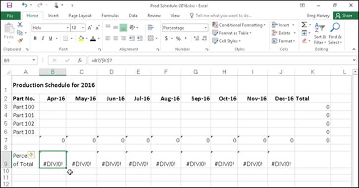
Figure 2-1: Blank 2016 Production Schedule spreadsheet that’s full of #DIV/0! errors.

The first percent-of-total formula in cell B9 contains the following:

=B7/$K$7

Because cell K7 with the grand total contains 0, the formula returns the #DIV/0! error value. Now, let me show you how to set a trap for the error in the logical_test argument inside an IF function. After the logical_test argument, you enter the value_if_true argument (which is 0 in this example) and the value_if_false argument (which is the B7/$K$7). With the addition of the IF function, the final formula looks like this:

=IF($K$7=0,0,B7/$K$7)

This formula then inputs 0 into cell B9, as shown in Figure 2-2, when the formula actually returns the #DIV/0! error value (because cell K7 is still empty or has a 0 in it), and the formula returns the percentage of total production when the formula doesn’t return the #DIV/0! error value (because cell K7 with the total production divisor is no longer empty or contains any other value besides 0). Next, all you have to do is copy this error-trapping formula in cell B9 over to J9 to remove all the #DIV/0! errors from this worksheet.

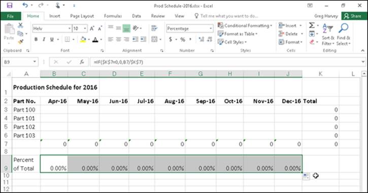
Figure 2-2: 2016 Production Schedule spreadsheet after trapping all the #DIV/0! errors.

The error-trapping formula created with the IF function in cell B9 works fine as long as you know that the grand total in cell K7 will contain either 0 or some other numerical value. It does not, however, trap any of the various error values, such as #REF! and #NAME?, nor does it account for the special #NA (Not Available) value. If, for some reason, one of the formulas feeding into the SUM formula in K8 returns one of these beauties, they will suddenly cascade throughout all the cells with the percent-of-total formulas (cell range B9:J9).

To trap all error values in the grand total cell K7 and prevent them from spreading to the percent-to-total formulas, you need to add the ISERROR function to the basic IF formula. The ISERROR function returns the logical value TRUE if the cell specified as its argument contains any type of error value, including the special #N/A value (if you use ISERR instead of ISERROR, it checks for all types of error values except for #N/A).

To add the ISERROR function, place it in the IF function as the logical_test argument. If, indeed, K7 does contain an error value or the #N/A value at the time the IF function is evaluated, you specify 0 as the value_if_true argument so that Excel inputs 0 in cell B9 rather than error value or #N/A. For the value_if_false argument, you specify the original IF function that inputs 0 if the cell K7 contains 0; otherwise, it performs the division that computes what percentage the April production figure is of the total production.

This amended formula with the ISERROR and two IF functions in cell B9 looks like this:

=IF(ISERROR($K$7),0,IF($K$7=0,0,B7/$K$7))

As soon as you copy this original formula to the cell range C9:J9, you’ve protected all the cells with the percent-of-total formulas from displaying and spreading any of those ugly error values.

Some people prefer to remove the display of zero values from any template that contains error-trapping formulas so that no one interprets the zeros as the correct value for the formula. To remove the display of zeros from a worksheet, deselect the Show a Zero in Cells That Have Zero Values check box in the Display Options for this Worksheet section of the Advanced tab of the Excel Options dialog box (File  ⇒  Options or Alt+FT). By this action, the cells with error-trapping formulas remain blank until you give them the data that they need to return the correct answers!

Whiting-Out Errors with Conditional Formatting

Instead of creating logical formulas to suppress the display of potential error values, you can use Conditional Formatting (see Book II, Chapter 2 for details) to deal with them. All you have to do is create a new conditional formatting rule that displays all potential error values in a white font (essentially, rendering them invisible in the cells of your worksheet). I think of using conditional formatting in this manner to deal with possible error values in a worksheet as applying a kind of electronic white-out that masks rather than suppresses formula errors.

To create this conditional formatting white-out for cells containing formulas that could easily be populated with error values, you follow these steps:

1. Select the ranges of cells with the formulas to which you want the new conditional formatting rule applied.

2. Select the Conditional Formatting button on the Home tab and then choose New Rule from its drop-down menu (Alt+HLN).

Excel displays the New Formatting Rule dialog box.

3. Select the Format Only Cells That Contain option in the Select a Rule Type section at the top of the New Formatting Rule dialog box.

4. Choose the Errors item from the Cell Value drop-down menu under Format Only Cells With section of the New Formatting Rule dialog box.

The New Formatting Rule dialog box now contains an Edit the Rule Description section at the bottom of the dialog box with Errors displayed under the Format Only Cells With heading.

5. Click the Format button to the immediate right of the Preview text box that now contains No Format Set.

Excel opens the Format Cells dialog box with the Font tab selected.

6. Click the Color drop-down menu button and then click the white swatch, the very first one on the color palette displayed under Theme Colors and then click OK.

Excel closes the Format Cells dialog box and the Preview text box in the New Formatting Rule dialog box now appears empty (as the No Format Set text is now displayed in a white font).

7. Select OK in the New Formatting Rule dialog box to close it and apply the new conditional formatting rule to your current cell selection.

After applying the new conditional formatting rule to a cell range, you can test it out by deliberately entering an error value into one of the cells referenced in one of the formulas in that range now covered by the “white-out” conditional formatting. Entering the #NA error value in one of these cells with the =NA( ) function is perhaps the easiest to do. Instead of seeing #NA values spread throughout the cell range, the cells should now appear empty because of the white font applied to all the #N/As, rendering them, for all intents and purposes, invisible.

Formula Auditing

If you don’t happen to trap those pesky error values before they get out into the spreadsheet, you end up having to track down the original cell that caused all the commotion and set it right. Fortunately, Excel offers some very effective formula-auditing tools for tracking down the cell that’s causing your error woes by tracing the relationships between the formulas in the cells of your worksheet. By tracing the relationships, you can test formulas to see which cells, called direct precedents in spreadsheet jargon, directly feed the formulas and which cells, calleddependents (nondeductible, of course), depend on the results of the formulas. Excel even offers a way to visually backtrack the potential sources of an error value in the formula of a particular cell.

The formula-auditing tools are found in the command buttons located in the Formula Auditing group on the Formulas tab of the Ribbon. These command buttons include the following:

· Trace Precedents: When you click this button, Excel draws arrows to the cells (the so-called direct precedents) that are referred to in the formula inside the selected cell. When you click this button again, Excel adds “tracer” arrows that show the cells (the so-called indirect precedents) that are referred to in the formulas in the direct precedents.

· Trace Dependents: When you click this button, Excel draws arrows from the selected cell to the cells (the so-called direct dependents) that use, or depend on, the results of the formula in the selected cell. When you click this button again, Excel adds tracer arrows identifying the cells (the so-called indirect dependents) that refer to formulas found in the direct dependents.

· Remove Arrows: Clicking this button removes all the arrows drawn, no matter what button or pull-down command you used to put them there. Click the drop-down button attached to this button to display a drop-down menu with three options: Remove Arrows to remove all arrows (just like clicking the Remove Arrows command button); Remove Precedent Arrows to get rid of the arrows that were drawn when you clicked the Trace Precedents button; and Remove Dependent Arrows to get rid of the arrows that were drawn when you clicked the Trace Dependents button.

· Show Formulas: To display all formulas in their cells in the worksheet instead of their calculated values — just like pressing Ctrl+` (tilde).

· Error Checking: When you click this button or click the Error Checking option on its drop-down menu, Excel displays the Error Checking dialog box, which describes the nature of the error in the current cell, gives you help on it, and enables you to trace its precedents. Choose the Trace Error option from this button’s drop-down menu to attempt to locate the cell that contains the original formula that has an error. Choose the Circular References option from this button’s drop-down menu to display a continuation menu with a list of all the cell addresses containing circular references in the active worksheet — click a cell address on this menu to select the cell with a circular reference formula in the worksheet. (See Book III, Chapter 1 for more on circular references in formulas.)

· Evaluate Formula: Clicking this button opens the Evaluate Formula dialog box, where you can have Excel evaluate each part of the formula in the current cell. The Evaluate Formula feature can be quite useful in formulas that nest many functions within them.

· Watch Window: Clicking this button opens the Watch Window dialog box, which displays the workbook, sheet, cell location, range name, current value, and formula in any cells that you add to the watch list. To add a cell to the watch list, click the cell in the worksheet, click the Add Watch button in the Watch Window dialog box, and then click Add in the Add Watch dialog box that appears.

Clicking the Trace Precedents and Trace Dependents buttons in the Formula Auditing group of the Formulas tab on the Ribbon lets you see the relationship between a formula and the cells that directly and indirectly feed it, as well as those cells that directly and indirectly depend on its calculation. Excel establishes this relationship by drawing arrows from the precedent cells to the active cell and from the active cell to its dependent cells.

If these cells are on the same worksheet, Excel draws solid red or blue arrows extending from each of the precedent cells to the active cell and from the active cell to the dependent cells. If the cells are not located locally on the same worksheet (they may be on another sheet in the same workbook or even on a sheet in a different workbook), Excel draws a black dotted arrow. This arrow comes from or goes to an icon picturing a miniature worksheet that sits to one side, with the direction of the arrowheads indicating whether the cells on the other sheet feed the active formula or are fed by it.

Tracing precedents

You can click the Trace Precedents command button on the Formulas tab of the Ribbon or press Alt+MP to trace all the generations of cells that contribute to the formula in the selected cell (kinda like tracing all the ancestors in your family tree). Figures 2-3 and 2-4 illustrate how you can use the Trace Precedents command button or its hot key equivalent to quickly locate the cells that contribute, directly and indirectly, to the simple addition formula in cell B9.

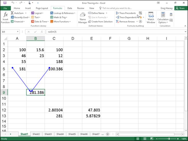
Figure 2-3: Clicking the Trace Precedents command button shows the direct precedents of the formula.

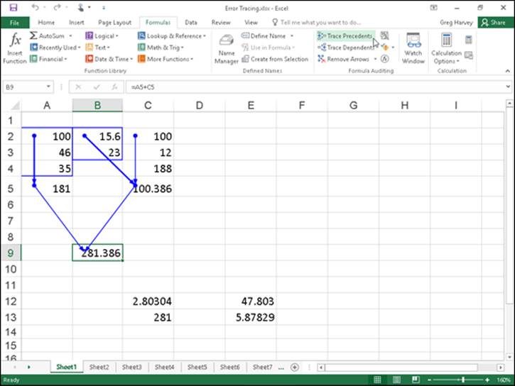
Figure 2-4: Clicking the Trace Precedents command button again shows the indirect precedents of the formula.

Figure 2-3 shows the worksheet after I clicked the Trace Precedents command button the first time. As you can see, Excel draws trace arrows from cells A5 and C5 to indicate that they are the direct precedents of the addition formula in cell B9.

In Figure 2-4, you see what happened when I clicked this command button a second time to display the indirect precedents of this formula. (Think of them as being a generation earlier in the family tree.) The new tracer arrows show that cells A2, A3, and A4 are the direct precedents of the formula in cell A5 — indicated by a border around the three cells. (Remember that cell A5 is the first direct precedent of the formula in cell B9.) Likewise, cells B2 and B3 as well as cell C2 are the direct precedents of the formula in cell C5. (Cell C5 is the second direct precedent of the formula in cell B9.)

Each time you click the Trace Precedents command button, Excel displays another (earlier) set of precedents, until no more generations exist. If you are in a hurry (as most of us are most of the time), you can speed up the process and display both the direct and indirect precedents in one operation by double-clicking the Trace Precedents command button. To clear the worksheet of tracer arrows, click the Remove Arrows command button on the Formulas tab.

Figure 2-5 shows what happened after I clicked the Trace Precedents command button a third time (after clicking it twice before, as shown in Figures 2-3 and 2-4). Clicking the command button reveals both the indirect precedents for cell C5. The formulas in cells B2 and C2 are the direct precedents of the formula in cell C5. The direct precedent of the formula in cell C2 (and, consequently, the indirect precedent of the one in cell C5) is not located on this worksheet. This fact is indicated by the dotted tracer arrow coming from that cute miniature worksheet icon sitting on top of cell A3.

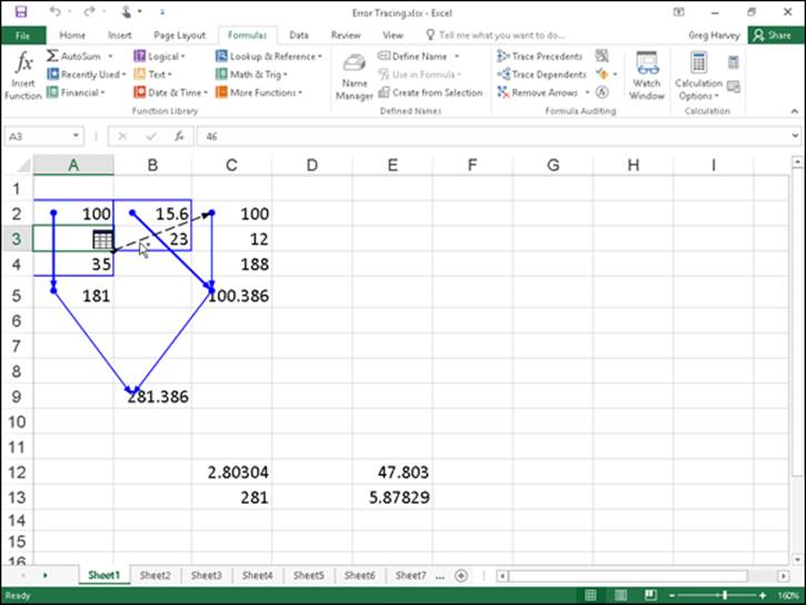
Figure 2-5: Clicking the Trace Precedents command button a third time shows a precedent on another worksheet.

To find out exactly which workbook, worksheet, and cell(s) hold the direct precedents of cell C2, I double-clicked somewhere on the dotted arrow. (Clicking the icon with the worksheet miniature doesn’t do a thing.) Double-clicking the dotted tracer arrow opens the Go To dialog box, which shows a list of all the precedents, including the workbook, worksheet, and cell references. To go to a precedent on another worksheet, double-click the reference in the Go To list box, or select it and click OK. (If the worksheet is in another workbook, this workbook file must already be open before you can go to it.)

The Go To dialog box, shown in Figure 2-6, displays the following direct precedent of cell C2, which is cell B4 on Sheet2 of the same workbook:

'[Error Tracing.xls]Sheet2'!$B$4

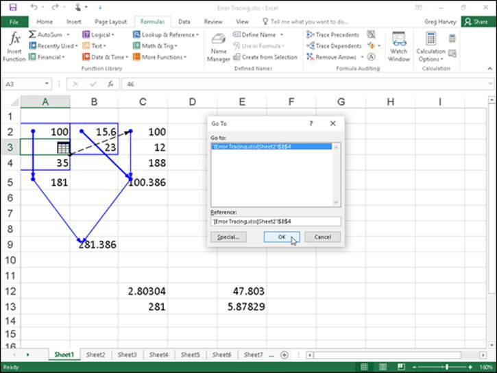
Figure 2-6: Double-clicking the dotted tracer arrow opens the Go To dialog box showing the location.

To jump directly to this cell, double-click the cell reference in the Go To dialog box.

You can also select precedent cells that are on the same worksheet as the active cell by double-clicking somewhere on the cell’s tracer arrow. Excel selects the precedent cell without bothering to open up the Go To dialog box.

You can use the Special button in the Go To dialog box (see Figure 2-6) to select all the direct or indirect precedents or the direct or indirect dependents that are on the same sheet as the formula in the selected cell. After opening the Go To dialog box (Ctrl+G or F5) and clicking the Special button, you simply click the Precedents or Dependents option button and then choose between the Direct Only and All Levels option buttons before you click OK.

Tracing dependents

You can click the Trace Dependents command button in the Formula Auditing group of the Formulas tab on the Ribbon or press Alt+MD to trace all the generations of cells that either directly or indirectly utilize the formula in the selected cell (kind of like tracing the genealogy of all your ancestors). Tracing dependents with the Trace Dependents command button is much like tracing precedents with the Trace Precedents command button. Each time you click this button, Excel draws another set of arrows that show a generation of dependents further removed. To display both the direct and indirect dependents of a cell in one fell swoop, double-click the Trace Dependents command button.

Figure 2-7 shows what happened after I selected cell B9 and then double-clicked the Trace Dependents command button on the Formulas tab of the Ribbon to display both the direct and indirect dependents and then clicked it a third time to display the dependents on another worksheet.

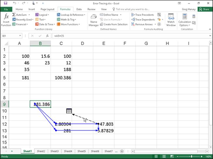
Figure 2-7: Clicking the Trace Dependents command button shows all the dependents of the formula in cell B9.

As this figure shows, Excel first draws tracer arrows from cell B9 to cells C12 and C13, indicating that C12 and C13 are the direct dependents of cell B9. Then, it draws tracer arrows from cells C12 and C13 to E12 and E13, respectively, the direct dependents of C12 and C13 and the indirect dependents of B9. Finally, it draws a tracer arrow from cell E12 to another sheet in the workbook (indicated by the dotted tracer arrow pointing to the worksheet icon).

Error checking

Whenever a formula yields an error value other than #N/A (refer to Table 2-1 for a list of all the error values) in a cell, Excel displays a tiny error indicator (in the form of the triangle) in the upper-left corner of the cell, and an alert options button appears to the left of that cell when you make it active. If you position the mouse or Touch pointer on that options button, a drop-down button appears to its right that you can click to display a drop-down menu, and a ScreenTip appears below describing the nature of the error value.

When you click the drop-down button, a menu appears, containing an item with the name of the error value followed by the following items:

· Help on This Error: Opens an Excel Help window with information on the type of error value in the active cell and how to correct it.

· Show Calculation Steps: Opens the Evaluate Formula dialog box where you can walk through each step in the calculation to see the result of each computation.

· Ignore Error: Bypasses error checking for this cell and removes the error alert and Error options button from it.

· Edit in Formula Bar: Activates Edit mode and puts the insertion point at the end of the formula on the Formula bar.

· Error Checking Options: Opens the Formulas tab of the Excel Options dialog box where you can modify the options used in checking the worksheet for formula errors. (See “Changing the Error Checking options” section that immediately follows for details.)

If you’re dealing with a worksheet that contains many error values, you can use the Error Checking command button (the one with the check mark on top of a red alert exclamation mark) in the Formula Auditing group on the Ribbon’s Formulas tab to locate each error.

When you click the Error Checking command button, Excel selects the cell with the first error value and opens the Error Checking dialog box (see Figure 2-8) that identifies the nature of the error value in the current cell.

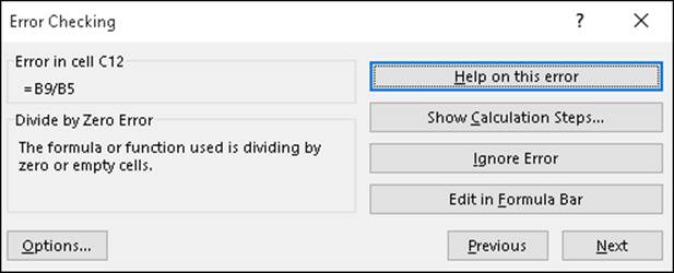
Figure 2-8: Flagging an error value in a worksheet in the Error Checking dialog box.

The command buttons in the Error Checking dialog box directly correspond to the menu options that appear when you click the cell’s alert options button (except that Error Checking Options on this drop-down menu is simply called the Options button in this dialog box).

In addition, the Error Checking dialog box contains Next and Previous buttons that you can click to have Excel select the cell with the next error value or return to the cell with the previously displayed error value.

Note that when you click the Next or Previous button when Excel has flagged the very first or last error value in the worksheet, the program displays an alert dialog box letting you know that the error check for the worksheet is complete. When you click the OK button, Excel closes both the alert dialog box and the Error Checking dialog box. Also note that clicking the Ignore Error button is the equivalent of clicking the Next button.

Changing the Error Checking options

When you choose Error Checking Options from the alert options drop-down menu attached to a cell with an error value or click the Options button in the Error Checking dialog box, Excel opens the Formulas tab of the Excel Options dialog box. This tab displays the Error Checking and Error Checking Rules options that are currently in effect in Excel. You can use these options on this Formulas tab to control when the worksheet is checked for errors and what cells are flagged:

· Enable Background Error Checking check box: Has Excel check your worksheets for errors when the computer is idle. When this check box is selected, you can change the color of the error indicator that appears as a tiny triangle in the upper-left corner of the cell (normally this indicator is green) by clicking a new color on the Indicate Errors Using This Color’s drop-down palette.

· Reset Ignored Errors button: Restores the error indicator and alert options button to all cells that you previously told Excel to ignore by choosing the Ignore Error item from the alert options drop-down menu attached to the cell.

· Indicate Errors Using This Color drop-down button: Enables you to select a particular color for cells containing error values from the drop-down palette that appears when you click this button.

· Cells Containing Formulas That Result in an Error check box: Has Excel insert the error indicator and adds the alert options button to all cells that return error values.

· Inconsistent Calculated Column Formula in Tables check box: Has Excel flag formulas in particular columns of cell ranges formatted as tables that vary in their computations from the other formulas in the column.

· Cells Containing Years Represented as 2 Digits check box: Has Excel flag all dates entered as text with just the last two digits of the year as errors by adding an error indicator and alert options button to their cells.

· Numbers Formatted as Text or Preceded by an Apostrophe check box: Has Excel flag all numbers entered as text as errors by adding an error indicator and alert options button to their cells.

· Formulas Inconsistent with Other Formulas in Region check box: Has Excel flag any formula that differs from the others in the same area of the worksheet as an error by adding an error indicator and alert options button to its cell.

· Formulas Which Omit Cells in a Region check box: Has Excel flag any formula that omits cells from the range that it refers to as an error by adding an error indicator and alert options button to its cell.

· Unlocked Cells Containing Formulas check box: Has Excel flag any formula whose cell is unlocked when the worksheet is protected as an error by adding an error indicator and alert options button to its cell. (See Book IV, Chapter 1 for information on protecting worksheets.)

· Formulas Referring to Empty Cells check box: Has Excel flag any formula that refers to blank cells as an error by adding an error indicator and alert options button to its cell.

· Data Entered in a Table Is Invalid check box: Has Excel flag any formulas for which you’ve set up Data Validation (see Book II, Chapter 1 for details) and that contain values outside of those defined as valid.

Error tracing

Tracing a formula’s family tree, so to speak, with the Trace Precedents and Trace Dependents command buttons on the Ribbon’s Formulas tab is fine, as far as it goes. However, when it comes to a formula that returns a hideous error value, such as #VALUE! or #NAME!, you need to turn to Excel’s trusty Trace Error option.

To select the Trace Error option in the current cell containing an untraced error value, choose the Trace Error option from the Error Checking command button’s drop-down menu or press Alt+MKE.

Selecting the Trace Error option is a lot like using both the Trace Precedents and the Trace Dependents command button options, except that the Trace Error option works only when the active cell contains some sort of error value returned by either a bogus formula or a reference to a bogus formula. In tracking down the actual cause of the error value in the active cell (remember that these error values spread to all direct and indirect dependents of a formula), Excel draws blue tracer arrows from the precedents for the original bogus formula and then draws red tracer arrows to all the dependents that contain error values as a result.

When Trace Error loses the trail

The Trace Error option finds errors along the path of a formula’s precedents and dependents until it finds either the source of the error or one of the following problems:

· It encounters a branch point with more than one error source. In this case, Excel doesn’t make a determination on its own as to which path to pursue.

· It encounters existing tracer arrows. Therefore, always click the Remove Arrows command button to get rid of trace arrows before you choose the Trace Error option from the Error Checking button’s drop-down menu.

· It encounters a formula with a circular reference. (See Book III, Chapter 1 for more on circular references.)

Figure 2-9 shows the sample worksheet after I made some damaging changes that left three cells — C12, E12, and E13 — with #DIV/0! errors (meaning that somewhere, somehow, I ended up creating a formula that is trying to divide by zero, which is a real no-no in the wonderful world of math). To find the origin of these error values and identify its cause, I clicked the Trace Error option on the Error Checking command button’s drop-down menu while cell E12 was the active cell to engage the use of Excel’s faithful old Trace Error feature.

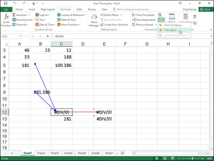
Figure 2-9: Using the Trace Error option to show the precedents and dependents of the formula.

You can see the results in Figure 2-9. Note that Excel has selected cell C12, although cell E12 was active when I selected the Trace Error option. To cell C12, Excel has drawn two blue tracer arrows that identify cells B5 and B9 as its direct precedents. From cell C12, the program has drawn a single red tracer arrow from cell C12 to cell E12 that identifies its direct dependent.

As it turns out, Excel’s Trace Error option is right on the money because the formula in cell C12 contains the bad apple rotting the whole barrel. I revised the formula in cell C12 so that it divided the value in cell B9 by the value in cell B5 without making sure that cell B5 first contained the SUM formula that totaled the values in the cell range B2:B4. The #DIV/0! error value showed up — remember that an empty cell contains a zero value as if you had actually entered 0 in the cell — and immediately spread to cells E12 and E13, which, in turn, use the value returned in C12 in their own calculations. Thus, these cells were infected with #DIV/0! error values as well.

As soon as you correct the problem in the original formula and thus get rid of all the error values in the other cells, Excel automatically converts the red tracer arrows (showing the proliferation trail of the original error) to regular blue tracer arrows, indicating merely that these restored cells are dependents of the formula that once contained the original sin. You can then remove all the tracer arrows from the sheet by clicking the Remove Arrows command button in the Formula Auditing group of the Ribbon’s Formulas tab (or by pressing Alt+MAA).

Evaluating a formula

The Evaluate Formula command button in the Formula Auditing group of the Ribbon’s Formulas tab (the one with fx inside a magnifying glass) opens the Evaluate Formula dialog box, where you can step through the calculation of a complicated formula to see the current value returned by each part of the calculation. This is often helpful in locating problems that prevent the formula from returning the hoped for or expected results.

To evaluate a formula step-by-step, position the cell pointer in that cell and then click the Evaluate Formula command button on the Formulas tab (or press Alt+MV). This action opens the Evaluate Formula dialog box with an Evaluation list box that displays the contents of the entire formula that’s in the current cell.

To have Excel evaluate the first expression or term in the formula (shown underlined in the Evaluation list box) and replace it with the currently calculated value, click the Evaluate button. If this expression uses an argument or term that is itself a result of another calculation, you can display its expression or formula by clicking the Step In button (see Figure 2-10) and then calculate its result by clicking the Evaluate button. After that, you can return to the evaluation of the expression in the original formula by clicking the Step Out button.

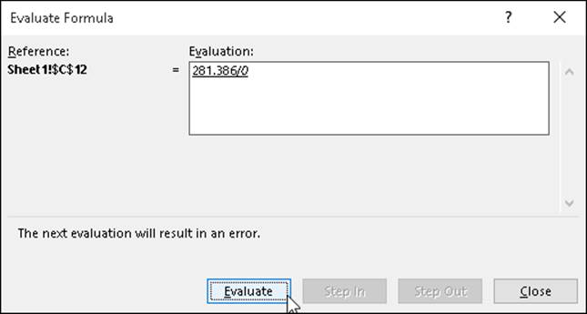
Figure 2-10: Calculating each part of a formula in the Evaluate Formula dialog box.

After you evaluate the first expression in the formula, Excel underlines the next expression or term in the formula (by using the natural order of precedence and a strict left-to-right order unless you have used parentheses to override this order), which you can then replace with its calculated value by clicking the Evaluate button. When you finish evaluating all the expressions and terms of the current formula, you can close the Evaluate Formula window by clicking its Close button in the upper-right corner of the window.

Instead of the Evaluate Formula dialog box, open the Watch Window dialog box by clicking the Watch Window button on the Formulas tab (Alt+MW) and add formulas to it when all you need to do is to keep an eye on the current value returned by a mixture of related formulas in the workbook. This enables you to see the effect that changing various input values has on their calculations (even when they’re located on different sheets of the workbook).

Removing Errors from the Printout

What if you don’t have the time to trap all the potential formula errors or track them down and eliminate them before you have to print out and distribute the spreadsheet? In that case, you may just have to remove the display of all the error values before you print the report.

To do this, click the Sheet tab in the Page Setup dialog box opened by clicking the Dialog Box launcher on the right side of the Page Setup group on the Page Layout tab. Click the Sheet tab in the Page Setup dialog box and then click the drop-down button attached to the Cell Errors As drop-down list box.

The default value for this drop-down list box is Displayed, meaning that all error values are displayed in the printout exactly as they currently appear in the worksheet. This drop-down list also contains the following items that you can click to remove the display of error values from the printed report:

· Click the <blank> option to replace all error values with blank cells.

· Click the - - option to replace all error values with two dashes.

· Click the #N/A option to replace all error values (except for #N/A entries, of course) with the special #N/A value (which is considered an error value when you select the <blank> or — options).

Blanking out error values or replacing them with dashes or #N/A values has no effect on them in the worksheet itself, only in any printout you make of the worksheet. You need to view the pages in the Print Preview area in the Print screen in the Backstage view (Ctrl+P) before you can see the effect of selecting an option besides the Displayed option in the Cell Errors As drop-down list box. Also, remember to reset the Cell Errors As option on the Sheet tab of the Page Setup dialog box back to the Displayed option when you want to print a version of the worksheet that shows the error values in all their cells in the worksheet printout.