CCNP Routing and Switching ROUTE 300-101 Official Cert Guide (2015)
Part II. IGP Routing Protocols
Chapter 8. The OSPF Link-State Database
This chapter covers the following topics:
![]() LSAs and the OSPF Link-State Database: This section examines LSA Types 1, 2, and 3 and describes how they allow OSPF routers to model a topology and choose the best routes for each known subnet.
LSAs and the OSPF Link-State Database: This section examines LSA Types 1, 2, and 3 and describes how they allow OSPF routers to model a topology and choose the best routes for each known subnet.
![]() The Database Exchange Process: This section details how neighboring routers use OSPF messages to exchange their LSAs.
The Database Exchange Process: This section details how neighboring routers use OSPF messages to exchange their LSAs.
![]() Choosing the Best Internal OSPF Routes: This section examines how OSPF routers calculate the cost for each possible route to each subnet.
Choosing the Best Internal OSPF Routes: This section examines how OSPF routers calculate the cost for each possible route to each subnet.
Open Shortest Path First (OSPF) and Enhanced Interior Gateway Routing Protocol (EIGRP) both use three major branches of logic, each of which populates a different table: the neighbor table, the topology table, or the IP routing table. This chapter examines topics related to the OSPF topology table—the contents and the processes by which routers exchange this information—and describes how OSPF routers choose the best routes in the topology table to be added to the IP routing table.
In particular, this chapter begins by looking at the building blocks of an OSPF topology table, namely, the OSPF link-state advertisement (LSA). Following that, the chapter examines the process by which OSPF routers exchange LSAs with each other. Finally, the last major section of the chapter discusses how OSPF chooses the best route among many when running the Shortest Path First (SPF) algorithm.
Note that this chapter focuses on OSPF version 2, the long-available version of OSPF that supports IPv4 routes. Chapter 9, “Advanced OSPF Concepts,” discusses OSPF version 3, which applies to IPv6.
“Do I Know This Already?” Quiz
The “Do I Know This Already?” quiz allows you to assess whether you should read the entire chapter. If you miss no more than one of these nine self-assessment questions, you might want to move ahead to the “Exam Preparation Tasks” section. Table 8-1 lists the major headings in this chapter and the “Do I Know This Already?” quiz questions covering the material in those headings so that you can assess your knowledge of those specific areas. The answers to the “Do I Know This Already?” quiz appear in Appendix A.
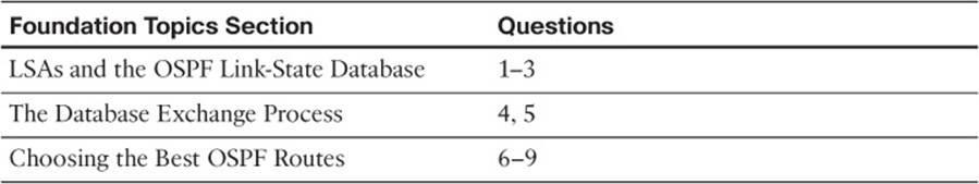
Table 8-1 “Do I Know This Already?” Foundation Topics Section-to-Question Mapping
1. A network design shows area 1 with three internal routers, area 0 with four internal routers, and area 2 with five internal routers. Additionally, one ABR (ABR1) connects areas 0 and 1, plus a different ABR (ABR2) connects areas 0 and 2. How many Type 1 LSAs would be listed in ABR2’s LSDB?
a. 6
b. 7
c. 15
d. 12
e. None of the other answers are correct.
2. A network planning diagram shows a large internetwork with many routers. The configurations show that OSPF has been enabled on all interfaces, IP addresses correctly configured, and OSPF working. For which of the following cases would you expect a router to create and flood aType 2 LSA?
a. When OSPF is enabled on a LAN interface, and the router is the only router connected to the subnet
b. When OSPF is enabled on a point-to-point serial link, and that router has both the higher router ID and higher interface IP address on the link
c. When OSPF is enabled on a Frame Relay point-to-point subinterface, has the lower RID and lower subinterface IP address, and otherwise uses default OSPF configuration on the interface
d. When OSPF is enabled on a working LAN interface on a router, and the router has been elected as a BDR
e. None of the other answers are correct.
3. A verification plan shows a network diagram with branch office Routers B1 through B100, plus two ABRs, ABR1 and ABR2, all in area 100. The branches connect to the ABRs using Frame Relay point-to-point subinterfaces. The verification plan lists the output of the show ip ospf database summary 10.100.0.0 command on a Router B1, one of the branches. Which of the following is true regarding the output that could be listed for this command?
a. The output lists nothing unless 10.100.0.0 has been configured as a summary route using the area range command.
b. If 10.100.0.0 is a subnet in area 0, the output lists one Type 3 LSA, specifically the LSA with the lower metric when comparing ABR1’s and ABR2’s LSA for 10.100.0.0.
c. If 10.100.0.0 is a subnet in area 0, the output lists two Type 3 LSAs, one each created by ABR1 and ABR2.
d. None, because the Type 3 LSAs would exist only in the ABR’s LSDBs.
4. Which of the following OSPF messages contains complete LSAs used during the database exchange process?
a. LSR
b. LSAck
c. LSU
d. DD
e. Hello
5. Routers R1, R2, R3, and R4 connect to the same 10.10.10.0/24 LAN-based subnet. OSPF is fully working in the subnet. Later, R5, whose OSPF priority is higher than the other four routers, joins the subnet. Which of the following are true about the OSPF database exchange process over this subnet at this point? (Choose two.)
a. R5 will send its DD, LSR, and LSU packets to the 224.0.0.5 all-DR-routers multicast address.
b. R5 will send its DD, LSR, and LSU packets to the 224.0.0.6 all-DR-routers multicast address.
c. The DR will inform R5 about LSAs by sending its DD, LSR, and LSU packets to the 224.0.0.6 all-SPF-routers multicast address.
d. The DR will inform R5 about LSAs by sending its DD, LSR, and LSU packets to the 224.0.0.5 all-SPF-routers multicast address.
6. R1 is internal to area 1, and R2 is internal to area 2. Subnet 10.1.1.0/24 exists in area 2 as a connected subnet off R2. ABR1 connects area 1 to backbone area 0, and ABR2 connects area 0 to area 2. Which of the following LSAs must R1 use when calculating R1’s best route for 10.1.1.0/24?
a. R2’s Type 1 LSA
b. Subnet 10.1.1.0/24’s Type 2 LSA
c. ABR1’s Type 1 LSA in area 0
d. Subnet 10.1.1.0/24’s Type 3 LSA in Area 0
e. Subnet 10.1.1.0/24’s Type 3 LSA in Area 1
7. Which of the following LSA types describe topology information that, when changed, requires a router in the same area to perform an SPF calculation? (Choose two.)
a. 1
b. 2
c. 3
d. 4
e. 5
f. 7
8. The following output was taken from Router R3. A scan of R3’s configuration shows that no bandwidth commands have been configured in this router. Which of the following answers list configuration settings that could be a part of a configuration that results in the following output? Note that only two of the three interface’s costs have been set directly. (Choose two.)
R3# show ip ospf interface brief
Interface PID Area IP Address/Mask Cost State Nbrs F/C
Se0/0/0.2 3 34 10.10.23.3/29 647 P2P 1/1
Se0/0/0.1 3 34 10.10.13.3/29 1000 P2P 1/1
Fa0/0 3 34 10.10.34.3/24 20 BDR 1/1
a. An auto-cost reference-bandwidth 1000 command in router ospf mode
b. An auto-cost reference-bandwidth 2000 command in router ospf mode
c. An ip ospf cost 1000 interface S0/0/0.1 command in router ospf mode
d. An auto-cost reference-bandwidth 64700 command in router ospf mode
9. Which of the following LSA types describe information related to topology or subnets useful for calculating routes for subnets inside the OSPF domain? (Choose three.)
a. 1
b. 2
c. 3
d. 4
e. 5
f. 7
Foundation Topics
LSAs and the OSPF Link-State Database
Every router that connects to a given OSPF area should learn the exact same topology data. Each router stores the data, composed of individual link-state advertisements (LSA), in its own copy of the link-state database (LSDB). Then, the router applies the Shortest Path First (SPF) algorithm to the LSDB to determine the best (lowest-cost) route for each reachable subnet (prefix/length).
When a router uses SPF to analyze the LSDB, the SPF process has some similarities to how humans put a jigsaw puzzle together—but without a picture of what the puzzle looks like. Humans faced with such a challenge might first look for the obvious puzzle pieces, such as the corner and edge pieces, because they are easily recognized. You might then group puzzle pieces together if they have the same color or look for straight lines that might span multiple puzzle pieces. And of course, you would be looking at the shapes of the puzzle pieces to see which ones fit together.
Similarly, a router’s SPF process must examine the individual LSAs and see how they fit together, based on their characteristics. To better appreciate the SPF process, the first section of this chapter examines the three LSA types that OSPF uses to describe an enterprise OSPF topology inside an OSPF domain. By understanding the types of LSAs, you can get a better understanding of what a router might look for to take the LSAs—the pieces of a network topology puzzle, if you will—and build the equivalent of a network diagram.
Table 8-2 lists the various OSPF LSA types. Not all of these LSA types are discussed in this chapter but are provided in the table as a convenience when studying.

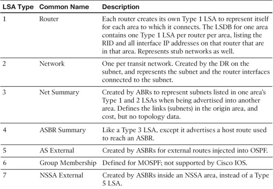
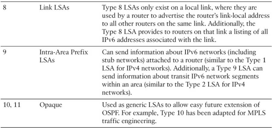
Table 8-2 OSPF LSA Types
LSA Type 1: Router LSA
An LSA type 1, called a Router LSA, identifies an OSPF router based on its OSPF router ID (RID). Each router creates a Type 1 LSA for itself and floods the LSA throughout the same area. To flood the LSA, the originating router sends the Type 1 LSA to its neighbors inside the same area, who in turn send it to their other neighbors inside the same area, until all routers in the area have a copy of the LSA.
Besides the RID of the router, this LSA also lists information about the attached links. In particular, the Type 1 LSA lists
![]() For each interface on which no designated router (DR) has been elected, it lists the router’s interface subnet number/mask and interface OSPF cost. (OSPF refers to these subnets as stub networks.)
For each interface on which no designated router (DR) has been elected, it lists the router’s interface subnet number/mask and interface OSPF cost. (OSPF refers to these subnets as stub networks.)
![]() For each interface on which a DR has been elected, it lists the IP address of the DR and a notation that the link attaches to a transit network (meaning that a Type 2 LSA exists for that network).
For each interface on which a DR has been elected, it lists the IP address of the DR and a notation that the link attaches to a transit network (meaning that a Type 2 LSA exists for that network).
![]() For each interface with no DR, but for which a neighbor is reachable, it lists the neighbor’s RID.
For each interface with no DR, but for which a neighbor is reachable, it lists the neighbor’s RID.
As with all OSPF LSAs, OSPF identifies a Type 1 LSA using a 32-bit link-state identifier (LSID). When creating its own Type 1 LSA, each router uses its own OSPF RID value as the LSID.
Internal routers each create a single Type 1 LSA for themselves, but area border routers (ABR) create multiple Type 1 LSAs for themselves: one per area. The Type 1 LSA in one area will list only interfaces in that area and only neighbors in that area. However, the router still has only a single RID, so all its Type 1 LSAs for a single router list the same RID. The ABR then floods each of its Type 1 LSAs into the appropriate area.
To provide a better backdrop for the upcoming LSA discussions, Figure 8-1 shows a sample internetwork, which will be used in most of the examples in this chapter.
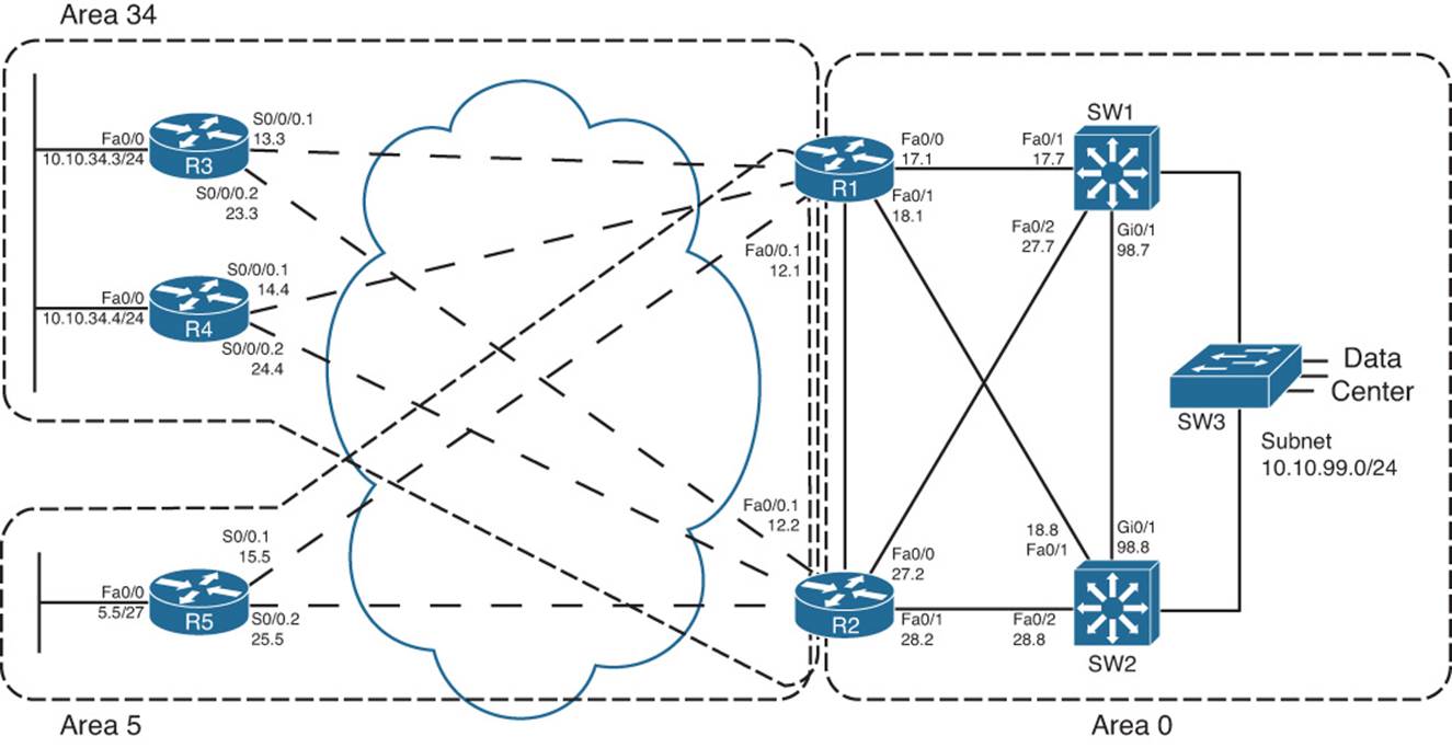
Figure 8-1 Sample OSPF Multiarea Design
Note
Unless otherwise noted, the first two octets of all networks in Figure 8-1 are 10.10, which are not shown to make the figure more readable.
All routers that participate in an area, be they internal routers or ABRs, create and flood a Type 1 LSA inside the area. For example, in Figure 8-1, area 5 has one internal router (R5, RID 5.5.5.5) and two ABRs: R1 with RID 1.1.1.1 and R2 with RID 2.2.2.2. Each of these three routers creates and floods its own Type 1 LSA inside area 5 so that all three routers know the same three Type 1 LSAs.
Next, to further understand the details inside a Type 1 LSA, first consider the OSPF configuration of R5 as an example. R5 has three IP-enabled interfaces: Fa0/0, S0/0.1, and S0/0.2. R5 uses point-to-point subinterfaces, so R5 should form neighbor relationships with both R1 and R2 with no extra configuration beyond enabling OSPF, in area 5, on all three interfaces. Example 8-1 shows this baseline configuration on R5.
Example 8-1 R5 Configuration—IP Addresses and OSPF
interface Fastethernet0/0
ip address 10.10.5.5 255.255.255.224
ip ospf 5 area 5
!
interface s0/0.1 point-to-point
ip address 10.10.15.5 255.255.255.248
frame-relay interface-dlci 101
ip ospf 5 area 5
!
interface s0/0.2 point-to-point
ip address 10.10.25.5 255.255.255.248
frame-relay interface-dlci 102
ip ospf 5 area 5
!
router ospf 5
router-id 5.5.5.5
!
R5# show ip ospf interface brief
Interface PID Area IP Address/Mask Cost State Nbrs F/C
se0/0.2 5 5 10.10.25.5/29 64 P2P 1/1
se0/0.1 5 5 10.10.15.5/29 64 P2P 1/1
fa0/0 5 5 10.10.5.5/27 1 DR 0/0
R5# show ip ospf neighbor
Neighbor ID Pri State Dead Time Address Interface
2.2.2.2 0 FULL/ - 00:00:30 10.10.25.2 Serial0/0.2
1.1.1.1 0 FULL/ - 00:00:38 10.10.15.1 Serial0/0.1
R5’s OSPF configuration enables OSPF, for process ID 5, placing three interfaces in area 5. As a result, R5’s Type 1 LSA will list at least these three interfaces as links, plus it will refer to the two working neighbors. Example 8-2 displays the contents of R5’s area 5 LSDB, including the detailed information in R5’s Type 1 LSA, including the following:
![]() The LSID of R5’s Type 1 LSA (5.5.5.5)
The LSID of R5’s Type 1 LSA (5.5.5.5)
![]() Three links that connect to a stub network, each listing the subnet/mask
Three links that connect to a stub network, each listing the subnet/mask
![]() Two links that state a connection to another router, one listing R1 (RID 1.1.1.1) and one listing R2 (RID 2.2.2.2)
Two links that state a connection to another router, one listing R1 (RID 1.1.1.1) and one listing R2 (RID 2.2.2.2)
Example 8-2 R5 Configuration—IP Addresses and OSPF
R5# show ip ospf database
OSPF Router with ID (5.5.5.5) (Process ID 5)
Router Link States (Area 5)
Link ID ADV Router Age Seq# Checksum Link count
1.1.1.1 1.1.1.1 835 0x80000002 0x006BDA 2
2.2.2.2 2.2.2.2 788 0x80000002 0x0082A6 2
5.5.5.5 5.5.5.5 787 0x80000004 0x0063C3 5
Summary Net Link States (Area 5)
Link ID ADV Router Age Seq# Checksum
10.10.12.0 1.1.1.1 835 0x80000001 0x00F522
10.10.12.0 2.2.2.2 787 0x80000001 0x00D73C
! lines omitted for brevity
R5# show ip ospf database router 5.5.5.5
OSPF Router with ID (5.5.5.5) (Process ID 5)
Router Link States (Area 5)
LS age: 796
Options: (No TOS-capability, DC)
LS Type: Router Links
Link State ID: 5.5.5.5
Advertising Router: 5.5.5.5
LS Seq Number: 80000004
Checksum: 0x63C3
Length: 84
Number of Links: 5
Link connected to: another Router (point-to-point)
(Link ID) Neighboring Router ID: 2.2.2.2
(Link Data) Router Interface address: 10.10.25.5
Number of TOS metrics: 0
TOS 0 Metrics: 64
Link connected to: a Stub Network
(Link ID) Network/subnet number: 10.10.25.0
(Link Data) Network Mask: 255.255.255.248
Number of TOS metrics: 0
TOS 0 Metrics: 64
Link connected to: another Router (point-to-point)
(Link ID) Neighboring Router ID: 1.1.1.1
(Link Data) Router Interface address: 10.10.15.5
Number of TOS metrics: 0
TOS 0 Metrics: 64
Link connected to: a Stub Network
(Link ID) Network/subnet number: 10.10.15.0
(Link Data) Network Mask: 255.255.255.248
Number of TOS metrics: 0
TOS 0 Metrics: 64
Link connected to: a Stub Network
(Link ID) Network/subnet number: 10.10.5.0
(Link Data) Network Mask: 255.255.255.224
Number of TOS metrics: 0
TOS 0 Metrics: 1
The first command, show ip ospf database, displays a summary of the LSAs known to R5. The output mainly consists of a single line per LSA, listed by LSA ID. The three highlighted lines of this output, in Example 8-2, highlight the RID of the three router (Type 1) LSAs, namely, 1.1.1.1 (R1), 2.2.2.2 (R2), and 5.5.5.5 (R5).
The output of the show ip ospf database router 5.5.5.5 command displays the detailed information in R5’s Router LSA. Looking at the highlighted portions, you see three stub networks—three interfaces on which no DR has been elected—and the associated subnet numbers. The LSA also lists the neighbor IDs of two neighbors (1.1.1.1 and 2.2.2.2) and the interfaces on which these neighbors can be reached.
Armed with the same kind of information in R1’s and R2’s Type 1 LSAs, a router has enough information to determine which routers connect, over which stub links, and then use the interface IP address configuration to figure out the interfaces that connect to the other routers. Figure 8-2shows a diagram of area 5 that could be built just based on the detailed information held in the Router LSAs for R1, R2, and R5.
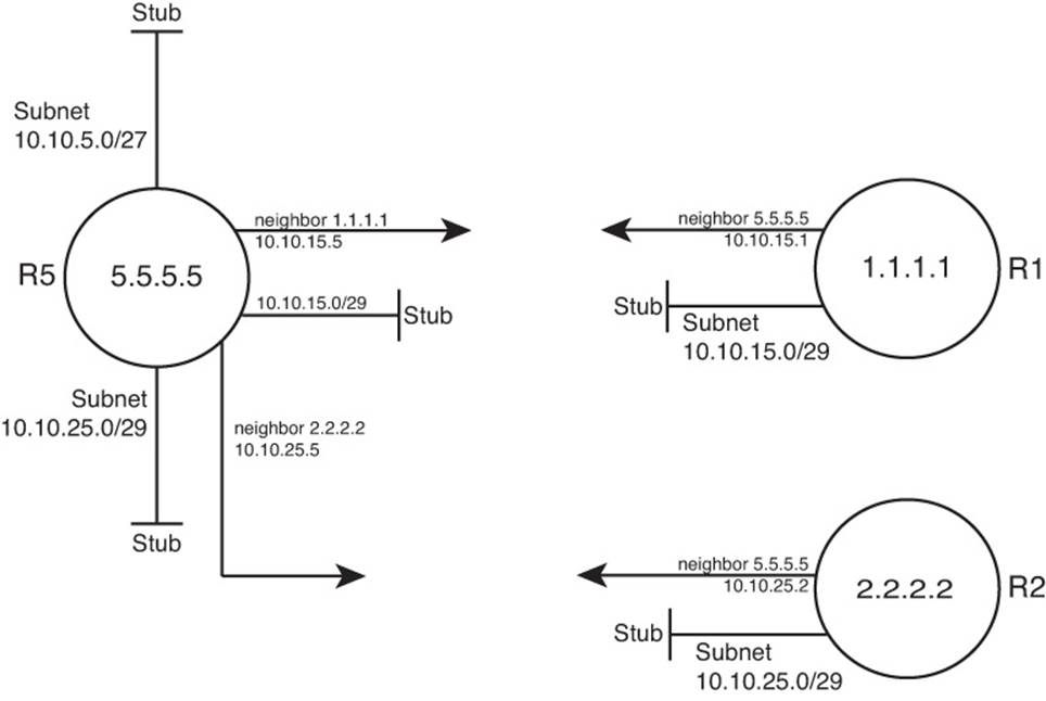
Figure 8-2 Three Type 1 LSAs in Area 5
Note that Figure 8-2 displays only information that could be learned from the Type 1 Router LSAs inside area 5. Each Type 1 Router LSA lists information about a router, but only the details related to a specific area. As a result, Figure 8-2 shows R1’s interface in area 5 but none of the interfaces in area 34 nor in area 0. To complete the explanation surrounding Figure 8-2, Example 8-3 lists R1’s Type 1 Router LSA for area 5.
Example 8-3 R1’s Type 1 LSA in Area 5
R5# show ip ospf database router 1.1.1.1
OSPF Router with ID (5.5.5.5) (Process ID 5)
Router Link States (Area 5)
Routing Bit Set on this LSA
LS age: 1306
Options: (No TOS-capability, DC)
LS Type: Router Links
Link State ID: 1.1.1.1
Advertising Router: 1.1.1.1
LS Seq Number: 80000002
Checksum: 0x6BDA
Length: 48
Area Border Router
Number of Links: 2
Link connected to: another Router (point-to-point)
(Link ID) Neighboring Router ID: 5.5.5.5
(Link Data) Router Interface address: 10.10.15.1
Number of TOS metrics: 0
TOS 0 Metrics: 64
Link connected to: a Stub Network
(Link ID) Network/subnet number: 10.10.15.0
(Link Data) Network Mask: 255.255.255.248
Number of TOS metrics: 0
TOS 0 Metrics: 64
Note
Because OSPF uses the RID for many purposes inside different LSAs—for example, as the LSID of a Type 1 LSA—Cisco recommends setting the RID to a stable, predictable value. To do this, use the OSPF router-id value OSPF subcommand or define a loopback interface with an IP address.
LSA Type 2: Network LSA
SPF requires that the LSDB model the topology with nodes (routers) and connections between nodes (links). In particular, each link must be between a pair of nodes. When a multiaccess data link exists—for example, a LAN—OSPF must somehow model that LAN so that the topology represents nodes and links between only a pair of nodes. To do so, OSPF uses the concept of a Type 2 Network LSA.
OSPF routers actually choose whether to use a Type 2 LSA for a multiaccess network based on whether a designated router (DR) has or has not been elected on an interface. So, before discussing the details of the Type 2 Network LSA, a few more facts about the concept of a DR need to be discussed.
Background on Designated Routers
As discussed in Chapter 7’s section “OSPF Network Types,” the OSPF network type assigned to a router interface tells that router whether to attempt to elect a DR on that interface. Then, when a router has heard a Hello from at least one other router, the routers elect a DR and BDR.
OSPF uses a DR in a particular subnet for two main purposes:
![]() To create and flood a Type 2 Network LSA for that subnet
To create and flood a Type 2 Network LSA for that subnet
![]() To aid in the detailed process of database exchange over that subnet
To aid in the detailed process of database exchange over that subnet
Routers elect a DR, and a backup DR (BDR), based on information in the OSPF Hello. The Hello message lists each router’s RID and a priority value. When no DR exists at the time, routers use the following election rules when neither a DR nor BDR yet exists:
![]() Choose the router with the highest priority (default 1, max 255, set with the ip ospf priority value interface subcommand).
Choose the router with the highest priority (default 1, max 255, set with the ip ospf priority value interface subcommand).
![]() If tied on priority, choose the router with highest RID.
If tied on priority, choose the router with highest RID.
![]() Choose a BDR, based on next-best priority, or if a tie, next-best (highest) RID.
Choose a BDR, based on next-best priority, or if a tie, next-best (highest) RID.
The preceding describes the election when no DR currently exists. However, the rules differ a bit when a DR and BDR already exist. After a DR and BDR are elected, no election is held until either the DR or BDR fails. If the DR fails, the BDR becomes the DR—regardless of whether a higher-priority router has joined the subnet—and a new election is held to choose a new BDR. If the BDR fails, a new election is held for the BDR, and the DR remains unchanged.
On LANs, the choice of DR matters little from a design perspective, but it does matter from an operational perspective. Throughout this chapter, note the cases in which the output of show commands identifies the DR and its role. Now, back to the topic of Type 2 LSAs.
Type 2 Network LSA Concepts
OSPF uses the concept of a Type 2 LSA to model a multiaccess network—a network with more than two routers connected to the same subnet—while still conforming to the “a link connects only two nodes” rule for the topology. For example, consider the network in Figure 8-3 (also shown as Figure 7-4 in the previous chapter). As seen in Chapter 7, “Fundamental OSPF Concepts,” all four routers form neighbor relationships inside area 0, with the DR and BDR becoming fully adjacent with the other routers.
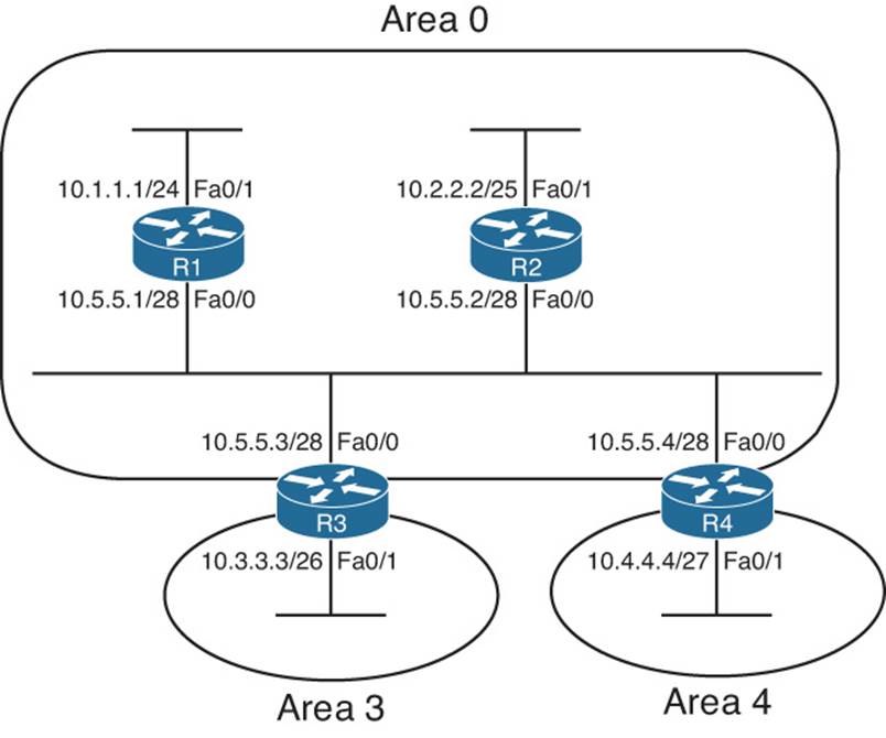
Figure 8-3 Small Network, Four Routers, on a LAN
OSPF cannot represent the idea of four routers connected through a single subnet by using a link connected to all four routers. Instead, OSPF defines the Type 2 Network LSA, used as a pseudonode. Each router’s Type 1 Router LSA lists a connection to this pseudonode, often called a transit network, which is then modeled by a Type 2 Network LSA. The Type 2 Network LSA itself then lists references back to each Type 1 Router LSA connected to it—four in this example, as shown in Figure 8-4.
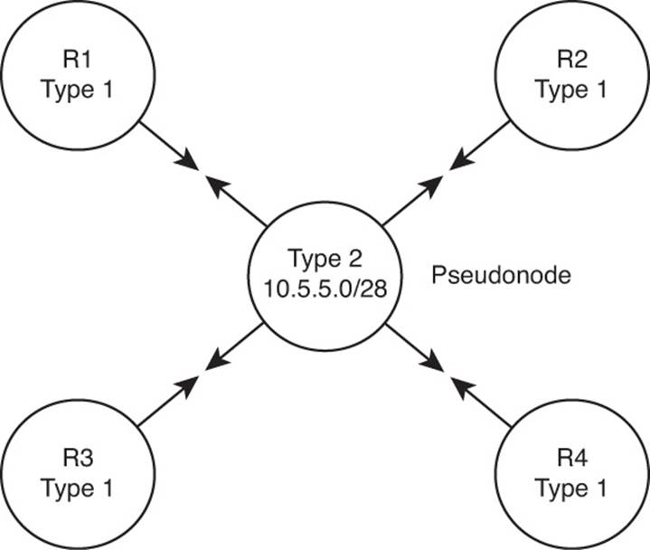
Figure 8-4 OSPF Topology When Using a Type 2 Network LSA
The elected DR in a subnet creates the Type 2 LSA for that subnet. The DR identifies the LSA by assigning an LSID of the DR’s interface IP address in that subnet. The Type 2 LSA also lists the DR’s RID as the router advertising the LSA.
Type 2 LSA show Commands
To see these concepts in the form of OSPF show commands, next consider area 34 back in Figure 8-1. This design shows that R3 and R4 connect to the same LAN, which means that a DR will be elected. (OSPF elects a DR on LANs when at least two routers pass the neighbor requirements and can become neighbors.) If both R3 and R4 default to use priority 1, R4 wins the election, because of its 4.4.4.4 RID (versus R3’s 3.3.3.3 RID). So, R4 creates the Type 2 LSA for that subnet and floods the LSA. Figure 8-5 depicts the area 34 topology, and Example 8-4 shows the related LSDB entries.
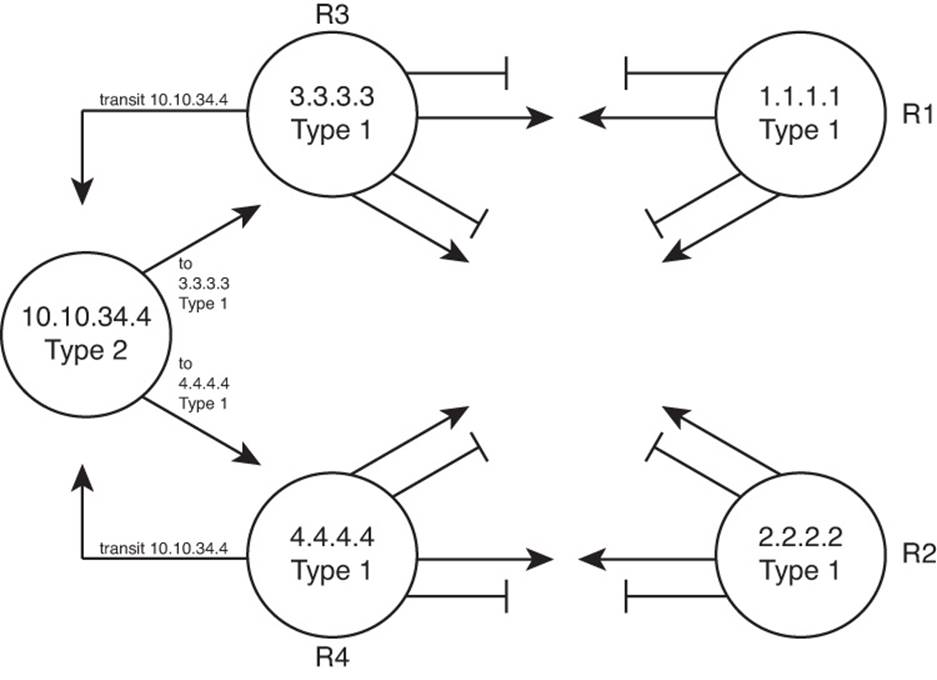
Figure 8-5 Area 34 Topology with Four Type 1 LSAs and One Type 2 LSA
Example 8-4 Area 34 LSAs for R3, Network 10.10.34.0 /24
R3# show ip ospf database
OSPF Router with ID (3.3.3.3) (Process ID 3)
Router Link States (Area 34)
Link ID ADV Router Age Seq# Checksum Link count
1.1.1.1 1.1.1.1 1061 0x80000002 0x00EA7A 4
2.2.2.2 2.2.2.2 1067 0x80000001 0x0061D2 4
3.3.3.3 3.3.3.3 1066 0x80000003 0x00E2E8 5
4.4.4.4 4.4.4.4 1067 0x80000003 0x007D3F 5
Net Link States (Area 34)
Link ID ADV Router Age Seq# Checksum
10.10.34.4 4.4.4.4 1104 0x80000001 0x00AB28
Summary Net Link States (Area 34)
Link ID ADV Router Age Seq# Checksum
10.10.5.0 1.1.1.1 1023 0x80000001 0x000BF2
10.10.5.0 2.2.2.2 1022 0x80000001 0x00EC0D
! lines omitted for brevity
R3# show ip ospf database router 4.4.4.4
OSPF Router with ID (3.3.3.3) (Process ID 3)
Router Link States (Area 34)
LS age: 1078
Options: (No TOS-capability, DC)
LS Type: Router Links
Link State ID: 4.4.4.4
Advertising Router: 4.4.4.4
LS Seq Number: 80000003
Checksum: 0x7D3F
Length: 84
Number of Links: 5
Link connected to: another Router (point-to-point)
(Link ID) Neighboring Router ID: 2.2.2.2
(Link Data) Router Interface address: 10.10.24.4
Number of TOS metrics: 0
TOS 0 Metrics: 64
Link connected to: a Stub Network
(Link ID) Network/subnet number: 10.10.24.0
(Link Data) Network Mask: 255.255.255.248
Number of TOS metrics: 0
TOS 0 Metrics: 64
Link connected to: another Router (point-to-point)
(Link ID) Neighboring Router ID: 1.1.1.1
(Link Data) Router Interface address: 10.10.14.4
Number of TOS metrics: 0
TOS 0 Metrics: 64
Link connected to: a Stub Network
(Link ID) Network/subnet number: 10.10.14.0
(Link Data) Network Mask: 255.255.255.248
Number of TOS metrics: 0
TOS 0 Metrics: 64
Link connected to: a Transit Network
(Link ID) Designated Router address: 10.10.34.4
(Link Data) Router Interface address: 10.10.34.4
Number of TOS metrics: 0
TOS 0 Metrics: 1
R3# show ip ospf database network 10.10.34.4
OSPF Router with ID (3.3.3.3) (Process ID 3)
Net Link States (Area 34)
Routing Bit Set on this LSA
LS age: 1161
Options: (No TOS-capability, DC)
LS Type: Network Links
Link State ID: 10.10.34.4 (address of Designated Router)
Advertising Router: 4.4.4.4
LS Seq Number: 80000001
Checksum: 0xAB28
Length: 32
Network Mask: /24
Attached Router: 4.4.4.4
Attached Router: 3.3.3.3
The show ip ospf database command lists a single line for each LSA. Note that the (highlighted) heading for Network LSAs lists one entry, with LSID 10.10.34.4, which is R4’s Fa0/0 IP address. The LSID for Type 2 Network LSAs is the interface IP address of the DR that creates the LSA.
The show ip ospf database router 4.4.4.4 command shows the new style of entry for the reference to a transit network, which again refers to a connection to a Type 2 LSA. The output lists an LSID of 10.10.34.4, which again is the LSID of the Type 2 LSA.
Finally, the show ip ospf database network 10.10.34.4 command shows the details of the Type 2 LSA, based on its LSID of 10.10.34.4. Near the bottom, the output lists the attached routers, based on RID. The SPF process can then use the cross-referenced information, as shown in Figure 8-5, to determine which routers connect to this transit network (pseudonode). The SPF process has information in both the Type 1 LSAs that refer to the transit network link to a Type 2 LSA, and the Type 2 LSA has a list of RIDs of Type 1 LSAs that connect to the Type 2 LSA, making the process of modeling the network possible.
OSPF can model all the topology inside a single area using Type 1 and 2 LSAs. When a router uses its SPF process to build a model of the topology, it can then calculate the best (lowest-cost) route for each subnet in the area. The next topic completes the LSA picture for internal OSPF routes by looking at Type 3 LSAs, which are used to model interarea routes.
LSA Type 3: Summary LSA
OSPF areas exist in part so that engineers can reduce the consumption of memory and compute resources in routers. Instead of having all routers, regardless of area, know all Type 1 and Type 2 LSAs inside an OSPF domain, ABRs do not forward Type 1 and Type 2 LSAs from one area into another area, and vice versa. This convention results in smaller per-area LSDBs, saving memory and reducing complexity for each run of the SPF algorithm, which saves CPU resources and improves convergence time.
However, even though ABRs do not flood Type 1 and Type 2 LSAs into other areas, routers still need to learn about subnets in other areas. OSPF advertises these interarea routes using the Type 3 Summary LSA. ABRs generate a Type 3 LSA for each subnet in one area, and advertise each Type 3 LSA into the other areas.
For example, if subnet A exists in area 3, the routers in area 3 learn of that subnet as part of Type 1 and Type 2 LSAs. However, an ABR connected to area 3 will not forward the Type 1 and Type 2 LSAs into other areas, instead creating a Type 3 LSA for each subnet (including subnet A). The routers inside the other areas can then calculate a route for the subnets (like subnet A) that exist inside another area.
Type 3 Summary LSAs do not contain all the detailed topology information, so in comparison to Types 1 and 2, these LSAs summarize the information—hence the name Summary LSA. Conceptually, a Type 3 LSA appears to be another subnet connected to the ABR that created and advertised the Type 3 LSA. The routers inside that area can calculate their best route to reach the ABR, which gives the router a good loop-free route to reach the subnet listed in a Type 3 LSA.
An example can certainly help in this case. First, consider the comparison shown in the top and bottom of Figure 8-6. The top depicts the topology shown back in Figure 8-1 if that design had used a single area. In that case, every router would have a copy of each Type 1 LSA (shown as a router name in the figure) and each Type 2 LSA (abbreviated as T2 in the figure). The bottom of Figure 8-6 shows the area 5 topology, when holding to the three-area design shown in Figure 8-1.
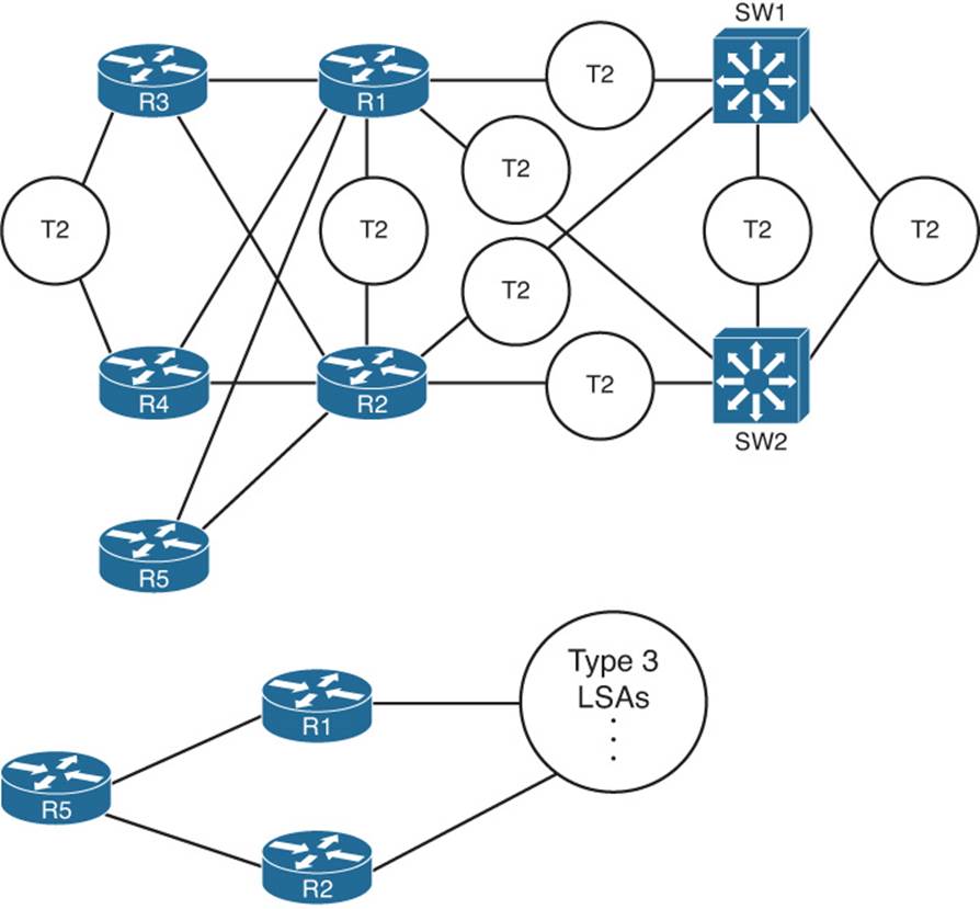
Figure 8-6 Comparing a Single-Area LSDB to a Three-Area LSDB
The ABR creates and floods each Type 3 LSA into the next area. The ABR assigns an LSID of the subnet address being advertised. It also adds its own RID to the LSA as well, so that routers know which ABR advertised the route. It also includes the subnet mask. The correlation between the advertising router’s RID and the LSID (subnet address) allows the OSPF processes to create the part of the topology as shown with Type 3 LSAs at the bottom of Figure 8-6.
Example 8-5 focuses on the Type 3 LSAs in area 34 of the network shown in Figure 8-1. Ten subnets exist outside area 34. As ABRs, both R1 and R2 create and flood a Type 3 LSA for each of these ten subnets, resulting in 20 Type 3 LSAs listed in the output of the show ip ospf databasecommand inside area 34. Then, the example focuses specifically on the Type 3 LSA for subnet 10.10.99.0/24.
Example 8-5 Type 3 LSAs in Area 34
R3# show ip ospf database
OSPF Router with ID (3.3.3.3) (Process ID 3)
Router Link States (Area 34)
Link ID ADV Router Age Seq# Checksum Link count
1.1.1.1 1.1.1.1 943 0x80000003 0x00E87B 4
2.2.2.2 2.2.2.2 991 0x80000002 0x005FD3 4
3.3.3.3 3.3.3.3 966 0x80000004 0x00E0E9 5
4.4.4.4 4.4.4.4 977 0x80000004 0x007B40 5
Net Link States (Area 34)
Link ID ADV Router Age Seq# Checksum
10.10.34.4 4.4.4.4 977 0x80000002 0x00A929
Summary Net Link States (Area 34)
Link ID ADV Router Age Seq# Checksum
10.10.5.0 1.1.1.1 943 0x80000002 0x0009F3
10.10.5.0 2.2.2.2 991 0x80000002 0x00EA0E
10.10.12.0 1.1.1.1 943 0x80000002 0x00F323
10.10.12.0 2.2.2.2 991 0x80000002 0x00D53D
10.10.15.0 1.1.1.1 943 0x80000002 0x0021BA
10.10.15.0 2.2.2.2 993 0x80000003 0x008313
10.10.17.0 1.1.1.1 946 0x80000002 0x00BC55
10.10.17.0 2.2.2.2 993 0x80000002 0x00A864
10.10.18.0 1.1.1.1 946 0x80000002 0x00B15F
10.10.18.0 2.2.2.2 994 0x80000002 0x009D6E
10.10.25.0 1.1.1.1 946 0x80000002 0x00355C
10.10.25.0 2.2.2.2 993 0x80000002 0x009439
10.10.27.0 1.1.1.1 946 0x80000002 0x0058AE
10.10.27.0 2.2.2.2 993 0x80000002 0x0030D3
10.10.28.0 1.1.1.1 947 0x80000002 0x004DB8
10.10.28.0 2.2.2.2 993 0x80000002 0x0025DD
10.10.98.0 1.1.1.1 946 0x80000002 0x004877
10.10.98.0 2.2.2.2 993 0x80000002 0x002A91
10.10.99.0 1.1.1.1 946 0x80000002 0x003D81
10.10.99.0 2.2.2.2 993 0x80000002 0x001F9B
R3# show ip ospf database summary 10.10.99.0
OSPF Router with ID (3.3.3.3) (Process ID 3)
Summary Net Link States (Area 34)
Routing Bit Set on this LSA
LS age: 1062
Options: (No TOS-capability, DC, Upward)
LS Type: Summary Links(Network)
Link State ID: 10.10.99.0 (summary Network Number)
Advertising Router: 1.1.1.1
LS Seq Number: 80000002
Checksum: 0x3D81
Length: 28
Network Mask: /24
TOS: 0 Metric: 2
Routing Bit Set on this LSA
LS age: 1109
Options: (No TOS-capability, DC, Upward)
LS Type: Summary Links(Network)
Link State ID: 10.10.99.0 (summary Network Number)
Advertising Router: 2.2.2.2
LS Seq Number: 80000002
Checksum: 0x1F9B
Length: 28
Network Mask: /24
TOS: 0 Metric: 2
Note
The Type 3 Summary LSA is not used for the purpose of route summarization. OSPF does support route summarization, and Type 3 LSAs might indeed advertise such a summary, but the Type 3 LSA does not inherently represent a summary route. The term Summary reflects the idea that the information is sparse compared to the detail inside Type 1 and Type 2 LSAs.
The upcoming section “Calculating the Cost of Interarea Routes” discusses how a router determines the available routes to reach subnets listed in a Type 3 LSA and how a router chooses which route is best.
Limiting the Number of LSAs
By default, Cisco IOS does not limit the number of LSAs that a router can learn. However, it might be useful to protect a router from learning too many LSAs to protect router memory. Also, with a large number of LSAs, the router might be unable to process the LSDB with SPF well enough to converge in a reasonable amount of time.
The maximum number of LSAs learned from other routers can be limited by a router using the max-lsa number OSPF subcommand. When configured, if the router learns more than the configured number of LSAs from other routers (ignoring those created by the router itself), the router reacts. The first reaction is to issue log messages. The router ignores the event for a time period, after which the router repeats the warning message. This ignore-and-wait strategy can proceed through several iterations, ending when the router closes all neighborships, discards its LSDB, and then starts adding neighbors again. (The ignore time, and the number of times to ignore the event, can be configured with the max-lsa command.)
Summary of Internal LSA Types
OSPF uses Type 1, 2, and 3 LSAs to calculate the best routes for all routes inside an OSPF routing domain. In a later chapter, we will explore Types 4, 5, and 7, which OSPF uses to calculate routes for external routes—routes redistributed into OSPF.
Table 8-3 summarizes some of the key points regarding OSPF Type 1, 2, and 3 LSAs. In particular for the ROUTE exam, the ability to sift through the output of various show ip ospf database commands can be important. Knowing what the OSPF LSID represents can help you interpret the output, and knowing the keywords used with the show ip ospf database lsa-type lsid commands can also be very useful. Table 8-3 summarizes these details.
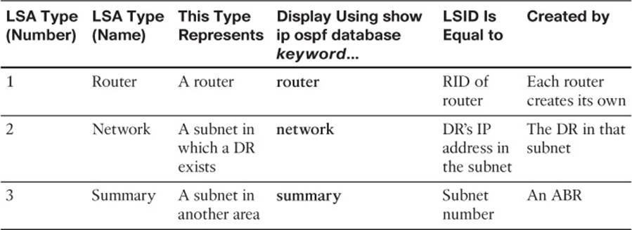
Table 8-3 Facts About LSA Types 1, 2, and 3
The Database Exchange Process
Every router in an area, when OSPF stabilizes after topology changes occur, should have an identical LSDB for that area. Internal routers (routers inside a single area) have only that area’s LSAs, but an ABR’s LSDB will contain LSAs for each area to which it connects. The ABR does, however, know which LSAs exist in each area.
OSPF routers flood both the LSAs they create, and the LSAs they learn from their neighbors, until all routers in the area have a copy of each of the most recent LSAs for that area. To manage and control this process, OSPF defines several messages, processes, and neighbor states that indicate the progress when flooding LSAs to each neighbor. This section begins by listing reference information for the OSPF messages and neighbor states. Next, the text describes the flooding process between two neighbors when a DR does not exist, followed by a description of the similar process used when a DR does exist. This section ends with a few items related to how routers avoid looping the LSA advertisements and how they periodically reflood the information.
OSPF Message and Neighbor State Reference
For reference, Table 8-4 lists the OSPF message types that will be mentioned in the next few pages. Additionally, Table 8-5 lists the various neighbor states. Although useful for study, when you are first learning this topic, feel free to skip these tables for now.
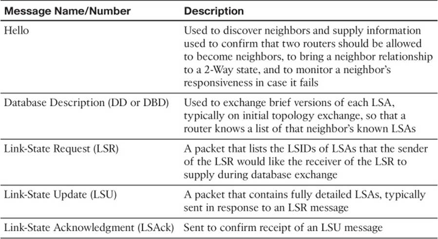
Table 8-4 OSPF Message Types and Functions
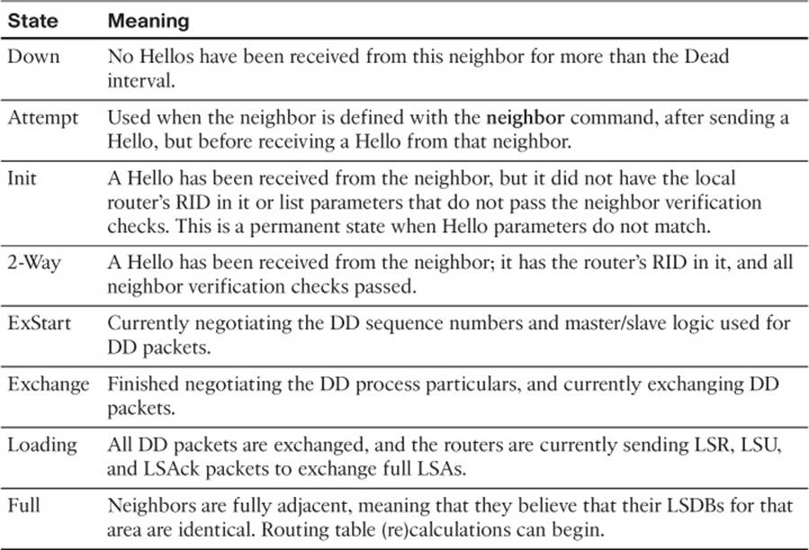
Table 8-5 OSPF Neighbor State Reference
Exchange Without a Designated Router
As discussed in Chapter 7, an OSPF interface’s network type tells a router whether to attempt to elect a DR on that interface. The most common case for which routers do not elect a DR occur on point-to-point topologies, such as true point-to-point serial links and point-to-point subinterfaces. This section examines the database exchange process on such interfaces, in preparation for the slightly more complex process when using a DR on an OSPF broadcast network type, like a LAN.
Each OSPF neighborship begins by exchanging Hellos until the neighbors (hopefully) reach the 2-Way state. During these early stages, the routers discover each other by sending multicast Hellos and then check each other’s parameters to make sure that all required items match (as listed inChapter 7’s Table 7-5). Figure 8-7 shows the details, with the various neighbor states listed on the outside of the figure and the messages listed in the middle.
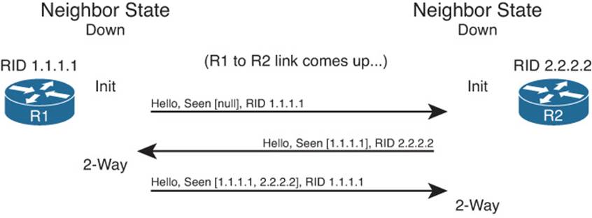
Figure 8-7 Neighbor Initialization—Early Stages
Figure 8-7 shows an example that begins with a failed neighborship, so the neighborship is in a down state. When a router tries to reestablish the neighborship, each router sends a multicast Hello and moves to an INIT state. After a router has both received a Hello and verified that all the required parameters agree, the router lists the other router’s RID in the Hello as being seen, as shown in the bottom two Hello messages in the figure. When a router receives a Hello that lists its own RID as having been seen by the other router, the router can transition to the 2-Way state.
When a router has reached the 2-Way state with a neighbor, as shown at the bottom of Figure 8-7, the router then decides whether it should exchange its LSDB entries. When no DR exists, the answer is always “yes.” Each router next follows this general process:
Step 1. Discover the LSAs known to the neighbor but unknown to me.
Step 2. Discover the LSAs known by both routers, but the neighbor’s LSA is more up to date.
Step 3. Ask the neighbor for a copy of all the LSAs identified in the first two steps.
Figure 8-8 details the messages and neighbor states used to exchange the LSAs between two neighbors. As with Figure 8-7, Figure 8-8 shows neighbor states on the outer edges of the flows (refer to Table 8-5 for reference). Routers display these neighbor states (with variants of the show ip ospf neighbor command), so a particular state can be useful in determining how far two neighbors have gotten in the database exchange process. The more important neighbor states will be mentioned throughout the chapter.
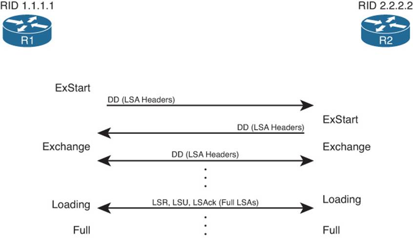
Figure 8-8 Overview of the Database Exchange Process Between Two Neighbors
The inner portions of Figure 8-8 represent the OSPF message flows, with Table 8-2, earlier in the chapter, listing the messages for reference. The next several pages examine the process shown in Figure 8-8 in more detail.
Discovering a Description of the Neighbor’s LSDB
After a router has decided to move forward from a 2-Way state and exchange its LSDB with a neighbor, the routers use the sequence shown in Figure 8-8. The next step in that process requires both routers to tell each other the LSIDs of all their known LSAs in that area. The primary goal is for each neighbor to realize which LSAs it does not know, so it can then ask for those full LSAs to be sent. To learn the list of LSAs known by a neighbor, the neighboring routers follow these steps:
Step 1. Multicast database description packets (abbreviated as both DD and DBD, depending on the reference) to 224.0.0.5, which is the all-SPF-routers multicast address.
Step 2. When sending the first DD message, transition to the ExStart state until one router, the one with the higher RID, becomes the master in a master/slave relationship.
Step 3. After electing a master, transition the neighbor to the Exchange state.
Step 4. Continue multicasting DD messages to each other until both routers have the same shared view of the LSIDs known collectively by both routers, in that area.
Note that the DD messages themselves do not list the entire LSAs, but rather just the LSA headers. These headers include the LSIDs of the LSAs and the LSA sequence number. The LS sequence number for an LSA begins at value 0x80000001 (hex) when initially created. The router creating the LSA increments the sequence number, and refloods the LSA, whenever the LSA changes. For example, if an interface moves from the up to down state, that router changes its Type 1 LSA to list that interface state as down, increments the LSA sequence number, and refloods the LSA.
The master router for each exchange controls the flow of DD messages, with the slave responding to the master’s DD messages. The master keeps sending DD messages until it lists all its known LSIDs in that area. The slave responds by placing LSA headers in its DD messages. Some of those LSA headers simply repeat what the slave heard from the master, for the purpose of acknowledging to the master that the slave learned that LSA header from the master. Additionally, the slave includes the LSA headers for any LSAs that the master did not list.
This exchange of DD messages ends with each router knowing a list of LSAs that it does not have in its LSDB, but the other router does have those LSAs. Additionally, each router also ends this process with a list of LSAs that the local router already knows, but for which the other router has a more recent copy (based on sequence numbers).
Exchanging the LSAs
When the two neighbors realize that they have a shared view of the list of LSIDs, they transition to the Loading state and start exchanging the full LSAs—but only those that they do not yet know about or those that have changed.
For example, when the two routers in Figure 8-8 first become neighbors, neither router will have a copy of the Type 1 LSA for the other router. So, R1 will request that R2 send its LSA with LSID 2.2.2.2. R2 will send its Type 1 LSA, and R1 will acknowledge receipt. The mechanics work like this:
Step 1. Transition the neighbor state to Loading.
Step 2. For any missing LSAs, send a Link-State Request (LSR) message, listing the LSID of the requested LSA.
Step 3. Respond to any LSR messages with a Link-State Update (LSU), listing one or more LSAs in each message.
Step 4. Acknowledge receipt by either sending a Link-State Acknowledgment (LSAck) message (called explicit acknowledgment) or by sending the same LSA that was received back to the other router in an LSU message (implicit acknowledgment).
Step 5. When all LSAs have been sent, received, and acknowledged, transition the neighborship to the FULL state (fully adjacent).
Note
Because this section examines the case without a DR, all these messages flow as multicasts to 224.0.0.5, the all SPF routers multicast address, unless the neighbors have been defined with an OSPF neighbor command.
By the end of this process, both routers should have an identical LSDB for the area to which the link has been assigned. At that point, the two routers can run the SPF algorithm to choose the currently best routes for each subnet.
Exchange with a Designated Router
Database exchange with a DR differs slightly than database exchange when no DR exists. The majority of the process is similar, with the same messages, meanings, and neighbor states. The big difference is the overriding choice of with whom each router chooses to perform database exchange.
Non-DR routers do not exchange their databases directly with all neighbors on a subnet. Instead, they exchange their database with the DR. Then, the DR exchanges any new/changed LSAs with the rest of the OSPF routers in the subnet.
The concept actually follows along with the idea of a Type 2 LSA as seen earlier in Figure 8-4. Figure 8-9 represents four Type 1 LSAs, for four real routers on the same LAN, plus a single Type 2 LSA that represents the multiaccess subnet. The DR created the Type 2 LSA as part of its role in life.
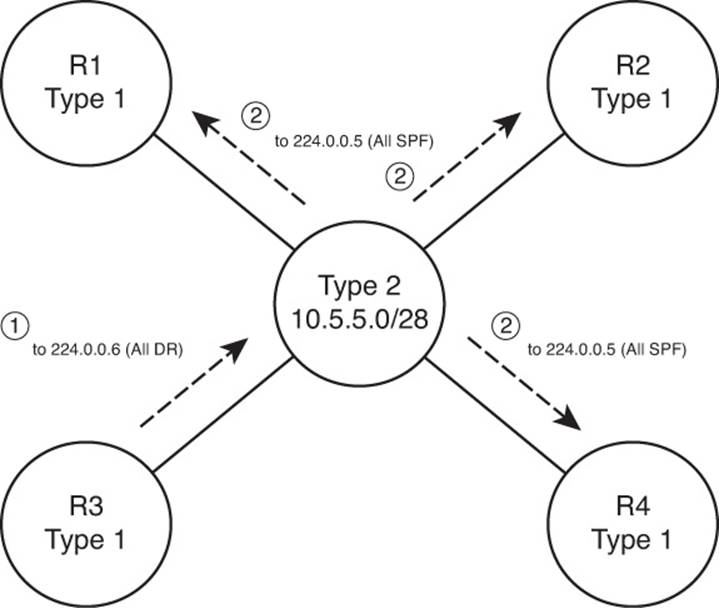
Figure 8-9 Conceptual View—Exchanging the Database with a Pseudonode
Figure 8-9 shows two conceptual steps for database exchange. The non-DR router (R3) first exchanges its database with the pseudonode, and then the Type 2 pseudonode exchanges its database with the other routers. However, the pseudonode is a concept, not a router. To make the process depicted in Figure 8-9 work, the DR takes on the role of the Type 2 pseudonode. The messages differ slightly as well, as follows:
![]() The non-DR performs database exchange with the same messages, as shown in Figure 8-9, but sends these messages to the 224.0.0.6 all-DR-routers multicast address.
The non-DR performs database exchange with the same messages, as shown in Figure 8-9, but sends these messages to the 224.0.0.6 all-DR-routers multicast address.
![]() The DR performs database exchange with the same messages but sends the messages to the 224.0.0.5 all-SPF-routers multicast address.
The DR performs database exchange with the same messages but sends the messages to the 224.0.0.5 all-SPF-routers multicast address.
Consider these two conventions one at a time. First, the messages sent to 224.0.0.6 are processed by the DR and the BDR only. The DR actively participates, replying to the messages, with the BDR acting as a silent bystander. In effect, this allows the non-DR router to exchange its database directly with the DR and BDR, but with none of the other routers in the subnet.
Next, consider the multicast messages from the DR to the 224.0.0.5 all-SPF-router multicast address. All OSPF routers process these messages, so the rest of the routers—the DROthers to use the Cisco IOS term—also learn the newly exchanged LSAs. This process completes the second step shown in the conceptual Figure 8-9, where the DR, acting like the pseudonode, floods the LSAs to the other OSPF routers in the subnet.
The process occurs in the background and can be generally ignored. However, for operating an OSPF network, an important distinction must be made. With a DR in existence, a DROther router performs the database exchange process (as seen in Figure 8-9) with the DR/BDR only and not any other DROther routers in the subnet. For example, in Figure 8-9, R1 acts as DR, R2 acts as BDR, and R3/R4 act as DROther routers. Because the underlying process does not make R3 and R4 perform database exchange with each other, the routers do not reach the FULL neighbor state, remaining in a 2-Way state.
Example 8-6 shows the resulting output for the LAN shown in Figure 8-9, with four routers. The output, taken from DROther R3, shows a 2-Way state with R4, the other DROther. It also shows on interface Fa0/0 that its own priority is 2. This output also shows a neighbor count (all neighbors) of 3 and an adjacent neighbor count (all fully adjacent neighbors) of 2, again because the neighborship between DROthers R3 and R4 is not a full adjacency.
Example 8-6 Demonstrating OSPF FULL and 2-Way Adjacencies
R3# show ip ospf interface fa0/0
FastEthernet0/0 is up, line protocol is up
Internet Address 172.16.1.3/24, Area 0
Process ID 75, Router ID 3.3.3.3, Network Type BROADCAST, Cost: 1
Transmit Delay is 1 sec, State DROTHER, Priority 2
Designated Router (ID) 1.1.1.1, Interface address 172.16.1.1
Backup Designated router (ID) 2.2.2.2, Interface address 172.16.1.2
Timer intervals configured, Hello 10, Dead 40, Wait 40, Retransmit 5
oob-resync timeout 40
Hello due in 00:00:02
Supports Link-local Signaling (LLS)
Cisco NSF helper support enabled
IETF NSF helper support enabled
Index 1/1, flood queue length 0
Next 0x0(0)/0x0(0)
Last flood scan length is 0, maximum is 4
Last flood scan time is 0 msec, maximum is 0 msec
Neighbor Count is 3, Adjacent neighbor count is 2
Adjacent with neighbor 1.1.1.1 (Designated Router)
Adjacent with neighbor 2.2.2.2 (Backup Designated Router)
Suppress hello for 0 neighbor(s)
R3# show ip ospf neighbor fa0/0
Neighbor ID Pri State Dead Time Address Interface
1.1.1.1 4 FULL/DR 00:00:37 172.16.1.1 FastEthernet0/0
2.2.2.2 3 FULL/BDR 00:00:37 172.16.1.2 FastEthernet0/0
44.44.44.44 1 2WAY/DROTHER 00:00:36 172.16.1.4 FastEthernet0/0
Flooding Throughout the Area
So far in this section, the database exchange process has focused on exchanging the database between neighbors. However, LSAs need to be flooded throughout an area. To do so, when a router learns new LSAs from one neighbor, that router then knows that its other neighbors in that same area might not know of that LSA. Similarly, when an LSA changes—for example, when an interface changes state—a router might learn the same old LSA but with a new sequence number, and again need to flood the changed LSA to other neighbors in that area.
Figure 8-10 shows a basic example of the process. In this case, R2, R3, and R4 have established neighbor relationships, with four LSAs in their LSDB in this area. R1 is again the new router added to the internetwork.
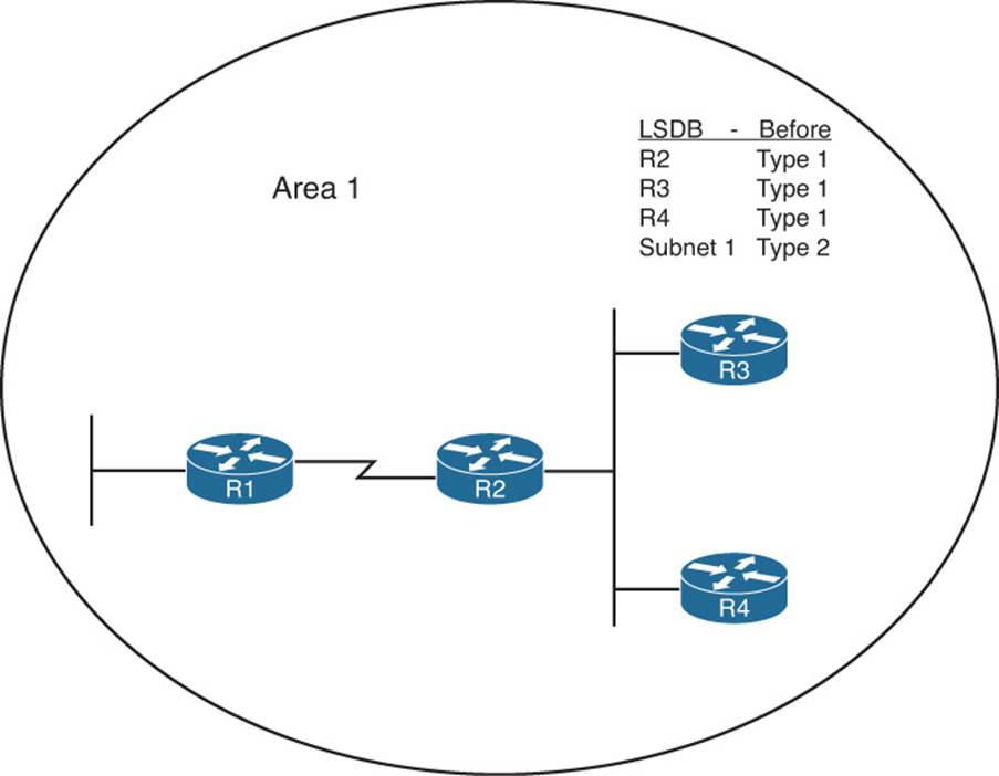
Figure 8-10 Flooding Throughout an Area
First, consider what happens as the new R1-R2 neighborship comes up and goes through database exchange. When R1 loads and the link comes up, R1 and R2 reach a full state and have a shared view of the area 1 LSDB. R2 has learned all R1’s new LSAs (should only be R1’s Type 1 Router LSA), and R1 has learned all the area 1 LSAs known to R2, including the Type 1 LSAs for R3 and R4.
Next, think about the LSDBs of R3 and R4 at this point. The database exchange between R1-R2 did not inform R3 or R4 about any of the new LSAs known by R1. So, R2, when it learns of R1’s Type 1 LSA, sends DD packets to the DR on the R2/R3/R4 LAN. LSR/LSU packets follow, resulting in R3 and R4 learning about the new LSA for R1. If more routers existed in area 1, the flooding process would continue throughout the entire area, until all routers know of the best (highest sequence number) copy of each LSA.
The flooding process prevents the looping of LSAs as a side effect of the database exchange process. Neighbors use DD messages to learn the LSA headers known by the neighbor, and then only request the LSAs known by the neighbor but not known by the local router. By requesting only unknown LSAs or new versions of old LSAs, routers prevent the LSA advertisements from looping.
Periodic Flooding
Although OSPF does not send routing updates on a periodic interval, as do distance vector protocols, OSPF does reflood each LSA every 30 minutes based on each LSA’s age variable. The router that creates the LSA sets this age to 0 (seconds). Each router then increments the age of its copy of each LSA over time. If 30 minutes pass with no changes to an LSA—meaning that no other reason existed in that 30 minutes to cause a reflooding of the LSA—the owning router increments the sequence number, resets the timer to 0, and refloods the LSA.
Because the owning router increments the sequence number and resets the LSAge every 1800 seconds (30 minutes), the output of various show ip ospf database commands should also show an age of less than 1800 seconds. For example, referring back to Example 8-5, the Type 1 LSA for R1 (RID 1.1.1.1) shows an age of 943 seconds and a sequence number of 0x80000003. Over time, the sequence number should increment once every 30 minutes, with the LSAge cycle upward toward 1800 and then back to 0 when the LSA is reflooded.
Note also that when a router realizes it needs to flush an LSA from the LSDB for an area, it actually sets the age of the LSA to the MaxAge setting (3600) and refloods the LSA. All the other routers receive the LSA, see that the age is already at the maximum, and cause those routers to also remove the LSA from their LSDBs.
Choosing the Best OSPF Routes
All this effort to define LSA types, create areas, and fully flood the LSAs has one goal in mind: to allow all routers in that area to calculate the best, loop-free routes for all known subnets. Although the database exchange process might seem laborious, the process by which SPF calculates the best routes requires a little less thought, at least to the level required for the CCNP ROUTE exam. In fact, the choice of the best route for a given subnet, and calculated by a particular router, can be summarized as follows:
![]() Analyze the LSDB to find all possible routes to reach the subnet.
Analyze the LSDB to find all possible routes to reach the subnet.
![]() For each possible route, add the OSPF interface cost for all outgoing interfaces in that route.
For each possible route, add the OSPF interface cost for all outgoing interfaces in that route.
![]() Pick the route with the lowest total cost.
Pick the route with the lowest total cost.
For humans, if you build a network diagram and note the OSPF cost for each interface (as shown with show ip ospf interface), you can easily add up the costs for each router’s possible routes to each subnet and tell which route OSPF will choose. The routers must use a more complex SPF algorithm to derive a mathematical model of the topology based on the LSAs. This section examines both the simpler human view of metric calculation and folds in some of the basics of what SPF must do on a router to calculate the best routes. It also goes through the options for tuning the metric calculation to influence the choice of routes.
OSPF Metric Calculation for Internal OSPF Routes
The process of calculating the cost from a router to each subnet might be intuitive to most people. However, spending a few minutes considering the details is worthwhile, in part to link the concepts with the LSAs, and to be better prepared for questions on the ROUTE exam. This section breaks the discussion into four sections: intra-area routes, interarea routes, a short discussion about cases when both intra-area and interarea routes exist for the same subnet, and an explanation of SPF calculations.
Calculating the Cost of Intra-Area Routes
When a router analyzes the LSDB to calculate the best route to each subnet, it does the following:
Step 1. Finds all subnets inside the area, based on the stub interfaces listed in the Type 1 LSAs and based on any Type 2 Network LSAs
Step 2. Runs SPF to find all possible paths through the area’s topology, from itself to each subnet
Step 3. Calculates the OSPF interface costs for all outgoing interfaces in each route, picking the lowest-total-cost route for each subnet as the best route
For example, Figure 8-11 shows the routers and links inside area 34, as a subset of the internetwork also shown in Figure 8-1. Figure 8-11 shows the interface numbers and OSPF costs.
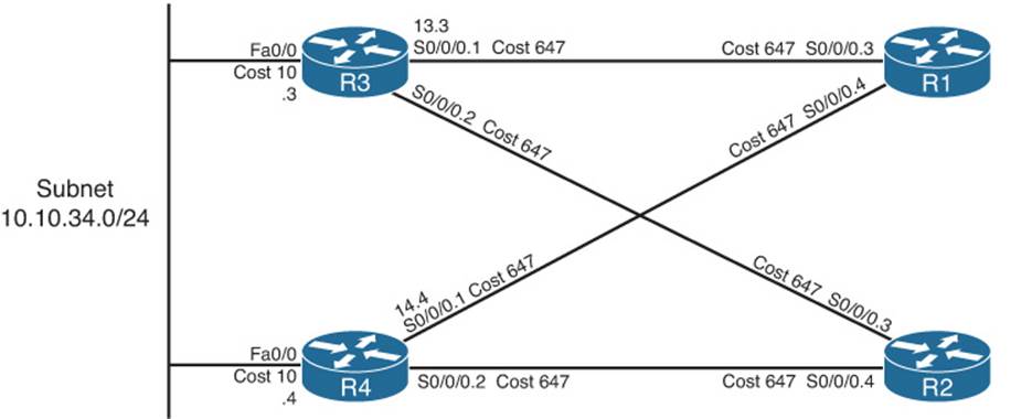
Figure 8-11 Area 34 Portion of Figure 8-1
Following the basic three-step process, at Step 1, R1 can determine that subnet 10.10.34.0/24 exists in area 34 because of the Type 2 LSA created by the DR in that subnet. For Step 2, R1 can then run SPF and determine four possible routes, two of which are clearly more reasonable to humans: R1-R3 and R1-R4. (The two other possible routes, R1-R3-R2-R4 and R1-R4-R2-R3, are possible and would be considered by OSPF but would clearly be higher cost.) For Step 3, R1 does the simple math of adding the costs of the outgoing interfaces in each route, as follows:
![]() R1-R3: Add R1’s S0/0/0.3 cost (647) and R3’s Fa0/0 cost (10), total 657
R1-R3: Add R1’s S0/0/0.3 cost (647) and R3’s Fa0/0 cost (10), total 657
![]() R1-R4: Add R1’s S0/0/0.4 cost (647) and R4’s Fa0/0 cost (10), total 657
R1-R4: Add R1’s S0/0/0.4 cost (647) and R4’s Fa0/0 cost (10), total 657
The metrics tie, so with a default setting of maximum-paths 4, R1 adds both routes to its routing table. Specifically, the routes list the metric of 657 and the next-hop IP address on the other end of the respective links: 10.10.13.3 (R3’s S0/0/0.1) and 10.10.14.4 (R4’s S0/0/0.1).
Note that OSPF supports equal-cost load balancing, but it does not support unequal-cost load balancing. The maximum-paths OSPF subcommand can be set as low as 1, with the maximum being dependent on router platform and Cisco IOS version. Modern Cisco IOS versions typically support 16 or 32 concurrent routes to one destination (maximum).
Calculating the Cost of Interarea Routes
From a human perspective, the cost for interarea routes can be calculated just like for intra-area routes if we have the full network diagram, subnet addresses, and OSPF interface costs. To do so, just find all possible routes from a router to the destination subnet, add up the costs of the outgoing interfaces, and choose the router with the lowest total cost.
However, OSPF routers cannot do the equivalent for interarea routes, because routers internal to one area do not have topological data—LSA Types 1 and 2—for other areas. Instead, ABRs create and flood Type 3 Summary LSAs into an area, listing the subnet address and mask, but not listing details about routers and links in the other areas. For example, Figure 8-12 shows both areas 34 and 0 from Figure 8-1, including interface costs. Then consider how OSPF determines the lowest-cost route from Router R3 for subnet 10.10.99.0/24, the data center subnet on the right.
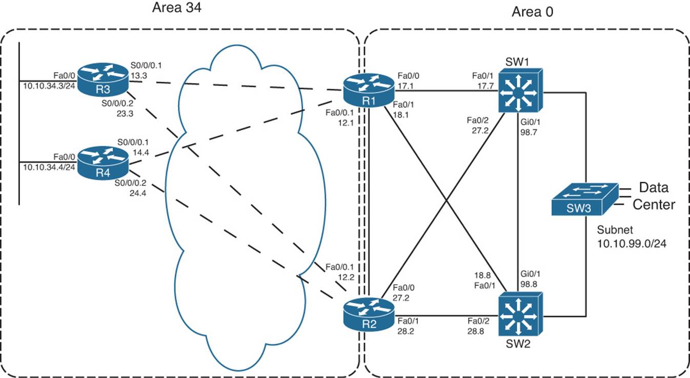
Figure 8-12 Area 34 and Area 0 Portion of Figure 8-1
R3 has a large number of possible routes to reach subnet 10.10.99.0/24. For example, just to get from R3 to R1, there are several possibilities: R3-R1, R3-R4-R1, and R3-R2-R1. From R1 the rest of the way to subnet 10.10.99.0/24, many more possibilities exist. The SPF algorithm has to calculate all possible routes inside an area to the ABR, so with more redundancy, SPF’s run time goes up. And SPF has to consider all the options, whereas we humans can rule out some routes quickly, because they appear to be somewhat ridiculous.
Because of the area design, with R1 and R2 acting as ABRs, R3 does not process all the topology shown in Figure 8-12. Instead, R3 relies on the Type 3 Summary LSAs created by the ABRs, which have the following information:
![]() The subnet number/mask represented by the LSA
The subnet number/mask represented by the LSA
![]() The cost of the ABR’s lowest-cost route to reach the subnet
The cost of the ABR’s lowest-cost route to reach the subnet
![]() The RID of the ABR
The RID of the ABR
Example 8-7 begins to examine the information that R3 will use to calculate its best route for subnet 10.10.99.0/24, on the right side of Figure 8-12. To see these details, Example 8-7 lists several commands taken from R1. It lists R1’s best route (actually two that tie) for subnet 10.10.99.0/24, with cost 11. It also lists the Type 3 LSA R1 generated by R1 for 10.10.99.0/24, again listing cost 11, and listing the Type 3 LSA created by ABR R2 and flooded into area 34.
Example 8-7 Route and Type 3 LSA on R1 for 10.10.99.0/24
R1# show ip route ospf
10.0.0.0/8 is variably subnetted, 15 subnets, 3 masks
O 10.10.5.0/27 [110/648] via 10.10.15.5, 00:04:19, Serial0/0/0.5
O 10.10.23.0/29 [110/711] via 10.10.13.3, 00:04:19, Serial0/0/0.3
O 10.10.24.0/29 [110/711] via 10.10.14.4, 00:04:19, Serial0/0/0.4
O 10.10.25.0/29 [110/711] via 10.10.15.5, 00:04:19, Serial0/0/0.5
O 10.10.27.0/24 [110/11] via 10.10.17.7, 00:04:19, FastEthernet0/0
[110/11] via 10.10.12.2, 00:04:19, FastEthernet0/0.1
O 10.10.28.0/24 [110/11] via 10.10.18.8, 00:04:19, FastEthernet0/1
[110/11] via 10.10.12.2, 00:04:19, FastEthernet0/0.1
O 10.10.34.0/24 [110/648] via 10.10.14.4, 00:04:19, Serial0/0/0.4
[110/648] via 10.10.13.3, 00:04:19, Serial0/0/0.3
O 10.10.98.0/24 [110/11] via 10.10.18.8, 00:04:19, FastEthernet0/1
[110/11] via 10.10.17.7, 00:04:19, FastEthernet0/0
O 10.10.99.0/24 [110/11] via 10.10.18.8, 00:04:19, FastEthernet0/1
[110/11] via 10.10.17.7, 00:04:19, FastEthernet0/0
R1# show ip ospf database summary 10.10.99.0
OSPF Router with ID (1.1.1.1) (Process ID 1)
! omitting output for area 5...
Summary Net Link States (Area 34)
LS age: 216
Options: (No TOS-capability, DC, Upward)
LS Type: Summary Links(Network)
Link State ID: 10.10.99.0 (summary Network Number)
Advertising Router: 1.1.1.1
LS Seq Number: 80000003
Checksum: 0x951F
Length: 28
Network Mask: /24
TOS: 0 Metric: 11
LS age: 87
Options: (No TOS-capability, DC, Upward)
LS Type: Summary Links(Network)
Link State ID: 10.10.99.0 (summary Network Number)
Advertising Router: 2.2.2.2
LS Seq Number: 80000002
Checksum: 0x7938
Length: 28
Network Mask: /24
TOS: 0 Metric: 11
Note
The examples use default bandwidth settings, but with all routers configured with the auto-cost reference-bandwidth 1000 command. This command is explained in the upcoming section “Changing the Reference Bandwidth.”
For routers in one area to calculate the cost of an interarea route, the process is simple when you realize that the Type 3 LSA lists the ABR’s best cost to reach that interarea subnet. To calculate the cost
Step 1. Calculate the intra-area cost from that router to the ABR listed in the Type 3 LSA.
Step 2. Add the cost value listed in the Type 3 LSA. (This cost represents the cost from the ABR to the destination subnet.)
A router applies these two steps for each possible route to reach the ABR. Following the example of Router R3 and subnet 10.10.99.0/24, Figure 8-13 shows the components of the calculation.
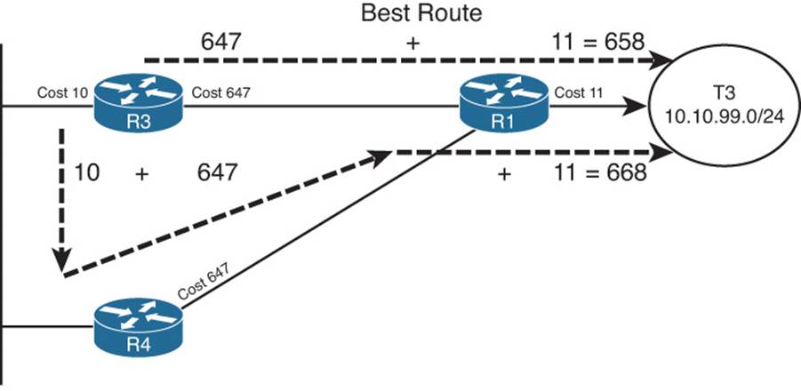
Figure 8-13 R3’s Calculation of Cost for 10.10.99.0/24
Figure 8-13 shows the calculation of both routes, with the intra-area cost to reach R1 either 647 or 657 in this case. For both routes, the cost listed in the Type 3 LSA sourced by R1, cost 11, is added.
When more than one ABR exists, as is the case as shown in Figure 8-12, each ABR should have created a Type 3 LSA for the subnet. In fact, the output in Example 8-7 showed the Type 3 LSA for 10.10.99.0/24 created by both R1 and another created by R2. For example, in the internetwork used throughout this chapter, ABRs R1 and R2 would create a Type 3 LSA for 10.10.99.0/24. So, in this particular example, R3 would also have to calculate the best route to reach 10.10.99.0/24 through ABR R2. Then, R3 would choose the best route among all routes for 10.10.99.0/24.
Each router repeats this process for all known routes to reach the ABR, considering the Type 3 LSAs from each ABR. In this case, R3 ties on metrics for one route through R1 and one through R2, so R3 adds both routes to its routing table, as shown in Example 8-8.
Example 8-8 Route and Type 3 LSA on R3 for 10.10.99.0/24
R3# show ip route 10.10.99.0 255.255.255.0
Routing entry for 10.10.99.0/24
Known via "ospf 3", distance 110, metric 658, type inter area
Last update from 10.10.13.1 on Serial0/0/0.1, 00:08:06 ago
Routing Descriptor Blocks:
* 10.10.23.2, from 2.2.2.2, 00:08:06 ago, via Serial0/0/0.2
Route metric is 658, traffic share count is 1
10.10.13.1, from 1.1.1.1, 00:08:06 ago, via Serial0/0/0.1
Route metric is 658, traffic share count is 1
R3# show ip route ospf
10.0.0.0/8 is variably subnetted, 15 subnets, 3 masks
O IA 10.10.5.0/27 [110/1304] via 10.10.23.2, 00:07:57, Serial0/0/0.2
[110/1304] via 10.10.13.1, 00:07:57, Serial0/0/0.1
O IA 10.10.12.0/24 [110/657] via 10.10.23.2, 00:08:17, Serial0/0/0.2
[110/657] via 10.10.13.1, 00:08:17, Serial0/0/0.1
! lines omitted for brevity
O IA 10.10.99.0/24 [110/658] via 10.10.23.2, 00:08:17, Serial0/0/0.2
[110/658] via 10.10.13.1, 00:08:17, Serial0/0/0.1
Besides the information that matches the expected outgoing interfaces per the figures, the output also flags these routes as interarea routes. The first command lists “type inter area” explicitly, and the show ip route ospf command lists the same information with the code “O IA,” meaning OSPF, interarea. Simply put, interarea routes are routes for which the subnet is known from a Type 3 Summary LSA.
Special Rules Concerning Intra-Area and Interarea Routes on ABRs
OSPF has a couple of rules concerning intra-area and interarea routes that take precedence over the simple comparison of the cost calculated for the various routes. The issue exists when more than one ABR connects to the same two areas. Many designs use two routers between the backbone and each nonbackbone area for redundancy, so this design occurs in many OSPF networks.
The issue relates to the fact that with two or more ABRs, the ABRs themselves, when calculating their own routing tables, can calculate both an intra-area route and interarea route for subnets in the backbone area. For example, consider the perspective of Router R1 from the last several examples, as depicted in Figure 8-14.
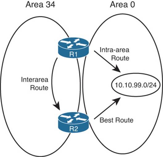
Figure 8-14 R1’s Choice: Intra-Area or Interarea Route to 10.10.99.0/24
Conceptually, R1 could calculate both the intra-area route and interarea route to 10.10.99.0/24. However, the OSPF cost settings could be set so that the lower-cost route for R1 actually goes through area 34, to ABR R2, and then on through area 0 to 10.10.99.0/24. However, two OSPF rules prevent such a choice by R1:
Step 1. When choosing the best route, an intra-area route is always better than a competing interarea route, regardless of metric.
Step 2. If an ABR learns a Type 3 LSA inside a nonbackbone area, the ABR ignores that LSA when calculating its own routes.
Because of the first rule, R1 would never choose the interarea route if the intra-area route were available. The second rule goes further, stating that R1 could never choose the interarea route—R1 simply ignores that LSA for the purposes of choosing its own best IP routes.
Metric and SPF Calculations
Before moving on to discuss how to influence route choices by changing the OSPF interface costs, first take a moment to consider the CPU-intensive SPF work done by a router. SPF does the work to piece together topology information to find all possible routes to a destination. As a result, SPF must execute when the intra-area topology changes, because changes in topology impact the choice of best route. However, changes to Type 3 LSAs do not drive a recalculation of the SPF algorithm, because the Type 3 LSAs do not actually describe the topology.
To take the analysis a little deeper, remember that an internal router, when finding the best interarea route for a subnet, uses the intra-area topology to calculate the cost to reach the ABR. When each route is identified, the internal router adds the intra-area cost to the ABR, plus the corresponding Type 3 LSA’s cost. A change to the Type 3 LSA—it fails, comes back up, or the metric changes—does impact the choice of best route, so the changed Type 3 LSA must be flooded. However, no matter the change, the change does not affect the topology between a router and the ABR—and SPF focuses on processing that topology data. So, only changes to Type 1 and 2 LSAs require an SPF calculation.
You can see the number of SPF runs, and the elapsed time since the last SPF run, using several variations of the show ip ospf command. Each time a Type 3 LSA changes and is flooded, SPF does not run, and the counter does not increment. However, each time a Type 1 or 2 LSA changes, SPF runs and the counter increments. Example 8-9 highlights the counter that shows the number of SPF runs on that router, in that area, and the time since the last run. Note that ABRs list a group of messages per area, showing the number of runs per area.
Example 8-9 Example with New Route Choices but No SPF Run
R3# show ip ospf | begin Area 34
Area 34
Number of interfaces in this area is 3
Area has no authentication
SPF algorithm last executed 00:41:02.812 ago
SPF algorithm executed 15 times
Area ranges are
Number of LSA 25. Checksum Sum 0x0BAC6B
Number of opaque link LSA 0. Checksum Sum 0x000000
Number of DCbitless LSA 0
Number of indication LSA 0
Number of DoNotAge LSA 0
Flood list length 0
Metric Tuning
Engineers have a couple of commands available that allow them to tune the values of the OSPF interface cost, thereby influencing the choice of best OSPF route. This section discusses the three methods: changing the reference bandwidth, setting the interface bandwidth, and setting the OSPF cost directly.
Changing the Reference Bandwidth
OSPF calculates the default OSPF cost for an interface based on the following formula:
Cost = Reference-Bandwidth / Interface-Bandwidth
The reference-bandwidth, which you can set using the auto-cost reference-bandwidth bandwidth router subcommand, sets the numerator of the formula for that one router, with a unit of Mbps. This setting can be different on different routers, but Cisco recommends using the same setting on all routers in an OSPF routing domain.
For example, serial interfaces default to a bandwidth setting of 1544, meaning 1544 kbps. The reference bandwidth defaults to 100, meaning 100 Mbps. After converting the reference bandwidth units to kbps (by multiplying by 1000) to match the bandwidth unit of measure, the cost, calculated per the defaults, for serial links would be
Cost = 100,000 / 1544 = 64
Note
OSPF always rounds down when the calculation results in a decimal value.
The primary motivation for changing the reference bandwidth is to accommodate good defaults for higher-speed links. With a default of 100 Mbps, the cost of Fast Ethernet interfaces is a cost value of 1. However, the minimum OSPF cost is 1, so Gigabit Ethernet and 10 Gigabit interfaces also then default to OSPF cost 1. By setting the OSPF reference bandwidth so that there is some difference in cost between the higher-speed links, OSPF can then choose routes that use those higher-speed interfaces.
Note
Although Cisco recommends that all routers use the same reference bandwidth, the setting is local to each router.
Note that in the examples earlier in this chapter, the bandwidth settings used default settings, but the auto-cost reference-bandwidth 1000 command was used on each router to allow different costs for Fast Ethernet and Gigabit interfaces.
Setting Bandwidth
You can indirectly set the OSPF cost by configuring the bandwidth speed interface subcommand (where speed is in kbps). In such cases, the formula shown in the previous section is used, just with the configured bandwidth value.
While on the topic of the interface bandwidth subcommand, a couple of seemingly trivial facts might matter to your choice of how to tune the OSPF cost. First, on serial links, the bandwidth defaults to 1544. On subinterfaces of those serial interfaces, the same bandwidth default is used.
On Ethernet interfaces, if not configured with the bandwidth command, the interface bandwidth matches the actual speed. For example, on an interface that supports autonegotiation for 10/100, the bandwidth is either 100,000 kbps (or 100 Mbps) or 10,000 kbps (or 10 Mbps), depending on whether the link currently runs at 100 or 10 Mbps, respectively.
Configuring Cost Directly
The most controllable method of configuring OSPF costs, but the most laborious, is to configure the interface cost directly. To do so, use the ip ospf cost value interface subcommand, substituting your chosen value as the last parameter.
Verifying OSPF Cost Settings
Several commands can be used to display the OSPF cost settings of various interfaces. Example 8-10 shows several, along with the configuration of all three methods for changing the OSPF cost. In this example, the following have been configured:
![]() The reference bandwidth is set to 1000.
The reference bandwidth is set to 1000.
![]() Interface S0/0/0.1 has its bandwidth set to 1000 kbps.
Interface S0/0/0.1 has its bandwidth set to 1000 kbps.
![]() Interface Fa0/0 has its cost set directly to 17.
Interface Fa0/0 has its cost set directly to 17.
Example 8-10 R3 with OSPF Cost Values Set
router ospf 3
auto-cost reference-bandwidth 1000
interface S0/0/0.1
bandwidth 1000
interface fa0/0
ip ospf cost 17
R3# show ip ospf interface brief
Interface PID Area IP Address/Mask Cost State Nbrs F/C
Se0/0/0.2 3 34 10.10.23.3/29 647 P2P 1/1
Se0/0/0.1 3 34 10.10.13.3/29 1000 P2P 1/1
Fa0/0 3 34 10.10.34.3/24 17 BDR 1/1
R3# show ip ospf interface fa0/0
FastEthernet0/0 is up, line protocol is up
Internet Address 10.10.34.3/24, Area 34
Process ID 3, Router ID 3.3.3.3, Network Type BROADCAST, Cost: 17
Enabled by interface config, including secondary ip addresses
Transmit Delay is 1 sec, State BDR, Priority 1
Designated Router (ID) 4.4.4.4, Interface address 10.10.34.4
Backup Designated router (ID) 3.3.3.3, Interface address 10.10.34.3
! lines omitted for brevity
Exam Preparation Tasks
Planning Practice
The CCNP ROUTE exam expects test takers to review design documents, create implementation plans, and create verification plans. This section provides some exercises that can help you to take a step back from the minute details of the topics in this chapter so that you can think about the same technical topics from the planning perspective.
For each planning practice table, simply complete the table. Note that any numbers in parentheses represent the number of options listed for each item in the solutions in Appendix F, “Completed Planning Practice Tables.”
Design Review Table
Table 8-6 lists several design goals related to this chapter. If these design goals were listed in a design document, and you had to take that document and develop an implementation plan, what implementation options come to mind? For any configuration items, a general description can be used, without concern about the specific parameters.
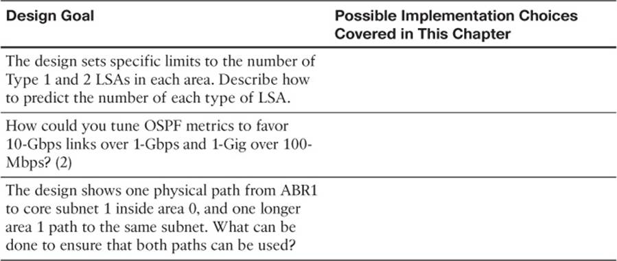
Table 8-6 Design Review
Implementation Plan Peer Review Table
Table 8-7 shows a list of questions that others might ask, or that you might think about, during a peer review of another network engineer’s implementation plan. Complete the table by answering the questions.
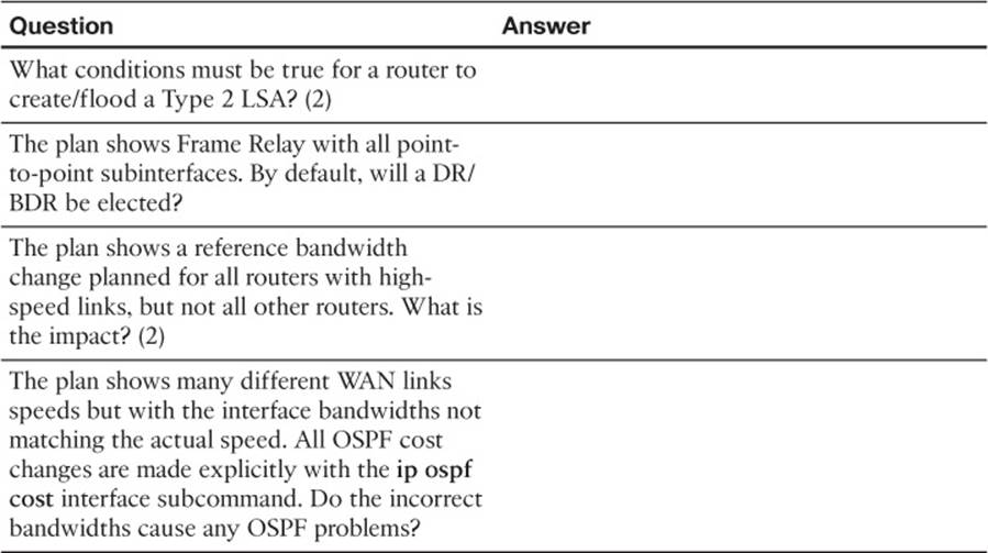
Table 8-7 Notable Questions from This Chapter to Consider During an Implementation Plan Peer Review
Create an Implementation Plan Table
To practice skills useful when creating your own OSPF implementation plan, list in Table 8-8 configuration commands related to the configuration of the following features. You might want to record your answers outside the book and set a goal to complete this table (and others like it) from memory during your final reviews before taking the exam.
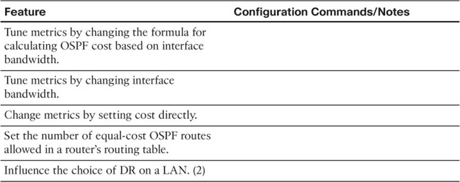
Table 8-8 Implementation Plan Configuration Memory Drill
Choose Commands for a Verification Plan Table
To practice skills useful when creating your own OSPF verification plan, list in Table 8-9 all commands that supply the requested information. You might want to record your answers outside the book and set a goal to complete this table (and others like it) from memory during your final reviews before taking the exam.
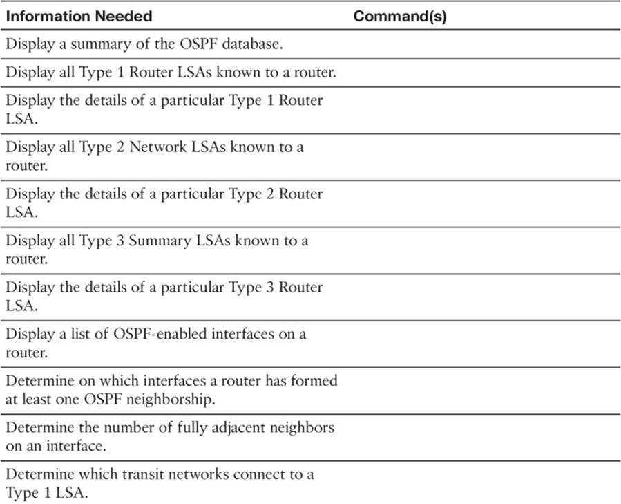
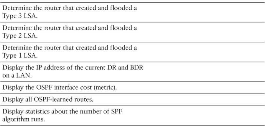
Table 8-9 Verification Plan Memory Drill
Note
Some of the entries in this table might not have been specifically mentioned in this chapter but are listed in this table for review and reference.
Review All the Key Topics
Review the most important topics from inside the chapter, noted with the Key Topic icon in the outer margin of the page. Table 8-10 lists a reference of these key topics and the page numbers on which each is found.
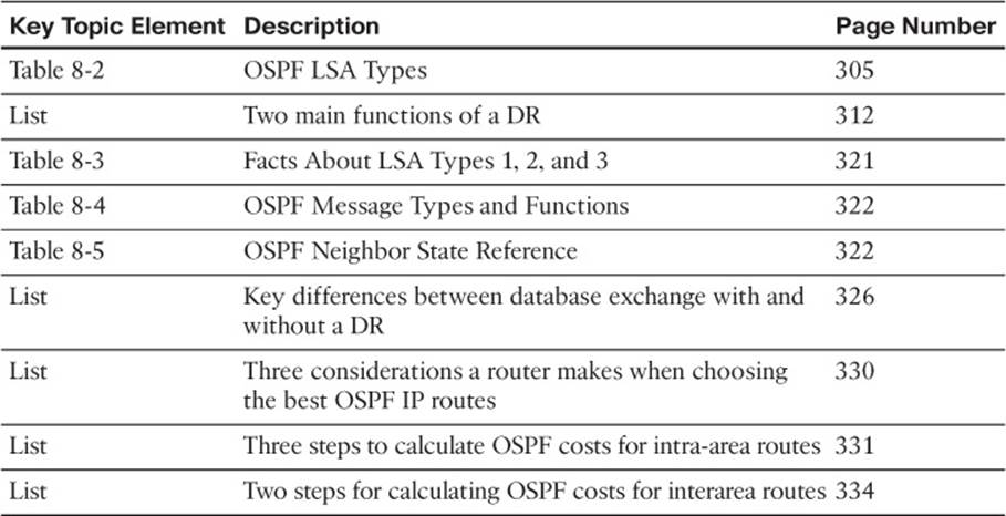
Table 8-10 Key Topics for Chapter 8
Complete the Tables and Lists from Memory
Print a copy of Appendix D, “Memory Tables,” (found on the CD) or at least the section for this chapter, and complete the tables and lists from memory. Appendix E, “Memory Tables Answer Key,” also on the CD, includes completed tables and lists to check your work.
Define Key Terms
Define the following key terms from this chapter, and check your answers in the glossary.
link-state identifier (LSID)
designated router (DR)
backup designated router (BDR)
internal router
area border router (ABR)
all-SPF-routers multicast
all-DR-routers multicast
link-state advertisement
Database Description (DD) packet
Link-State Request (LSR) packet
Link-State Acknowledgment (LSA) packet
Link-State Update (LSU) packet
Router LSA
Network LSA
Summary LSA
Type 1 LSA
Type 2 LSA
Type 3 LSA
reference bandwidth
SPF calculation
All materials on the site are licensed Creative Commons Attribution-Sharealike 3.0 Unported CC BY-SA 3.0 & GNU Free Documentation License (GFDL)
If you are the copyright holder of any material contained on our site and intend to remove it, please contact our site administrator for approval.
© 2016-2026 All site design rights belong to S.Y.A.