SQL Server Integration Services Design Patterns, Second Edition (2014)

Chapter 11. Data Warehouse Patterns

SQL Server Integration Services is an excellent all-purpose ETL tool. Because of its versatility, it is used by DBAs, developers, BI professionals, and even business principals in many different scenarios. Sometimes it’s a dump truck, used for the wholesale movement of enormous amounts of data. Other times it’s more like a scalpel, carving out with precision just the right amount of data.

Though it is a great tool in other areas, SSIS truly excels when used as a data warehouse ETL tool. It would be hard to argue that data warehousing isn’t its primary purpose in life. From native slowly changing dimension (SCD) elements to recently added CDC processing tasks and components, SSIS has all the hooks it needs to compete with data warehouse ETL tools at much higher price points.

In this chapter, we’ll discuss design patterns applicable to loading a data warehouse using SQL Server Integration Services. From incremental loads to error handling and general workflow, we’ll investigate methodologies and best practices that can be applied in SSIS data warehouse ETL.

Incremental Loads

Anyone who has spent more than ten minutes working in the data warehouse space has heard the term incremental loa d. Before we demonstrate design patterns for performing incremental loads, let’s first touch on the need for an incremental load.

What Is an Incremental Load?

As the name implies, an incremental load is one that processes a partial set of data based only on what is new or changed since the last execution. Although many consider incremental loads to be purely time based (for example, grabbing just the data processed on the prior business day), it’s not always that simple. Sometimes, changes are made to historical data that should be reflected in downstream systems, and unfortunately it’s not always possible to detect when changes were made. (As an aside, those ubiquitous “last update timestamp” fields are notorious for being wrong.)

Handling flexible data warehouse structures that allow not only inserts, but updates as well, can be a challenging proposition. In this chapter, we’ll surface a few design patterns in SSIS that you can use when dealing with changing data in your data warehouse.

Why Incremental Loads?

Imagine you are hired by a small shoe store to create a system through which the staff can analyze their sales data. Let’s say the store averages 50 transactions a day, amounting to an average of 100 items (2 items per transaction). If you do simple math on the row counts generated by the business, you’ll end up with fewer than 200 rows of data per day being sent to the analysis system. Even over the course of the entire year, you’re looking at less than 75,000 rows of data. With such a small volume of data, why would you want to perform an incremental load? After all, it would be almost as efficient to simply dump and reload the entire analytical database each night rather than try to calculate which rows are new, changed, or deleted.

In a situation like the one just described, the best course of action might be to perform a full load each day. However, in the real world, few, if any, systems are so small and simple. In fact, it’s not at all uncommon for data warehouse developers to work in environments that generate millions of rows of data per day. Even with the best hardware money can buy, attempting to perform a daily full load on that volume of data simply isn’t practical. The incremental load seeks to solve this problem by allowing the systematic identification of data to be moved from transactional systems to the data warehouse. By selectively carving out only the data that requires manipulation—specifically, the rows that have been inserted, updated, or deleted since the last load—we can eliminate a lot of unnecessary and duplicate data processing.

The Slowly Changing Dimension

When you consider the application of incremental data loads in a data warehouse scenario, there’s no better example than the slowly changing dimension (SCD). The nature of dimensional data is such that it often does require updates by way of manipulating existing rows in the dimension table (SCD Type 1) or expiring the current record and adding a new row for that value, thus preserving the history for that dimension attribute (SCD Type 2).

Although the slowly changing dimension is certainly not the only data warehouse structure to benefit from an incremental load, it is one of the most common species of that animal. As such, we’ll focus mostly on SCD structures for talking points around incremental loads.

Incremental Loads of Fact Data

Some data warehouse scenarios require the changing of fact data after it has been loaded to the data warehouse. This scenario is typically handled through a secondary load with a negating entry and a delta record, but some designs require the original fact record to be corrected.

In such cases, the same methodology used for SCD data may also apply to fact data. However, pay careful consideration to performance when applying SCD methods to fact data. Fact data is exponentially more voluminous than dimension data and typically involves millions, and sometimes billions, of records. Therefore, apply the SCD pattern to fact data only if you must. If there’s any flexibility at all in the data warehouse (DW) design, use the delta record approach instead.

Incremental Loads in SSIS

Microsoft SQL Server, and SSIS specifically, have several tools and methodologies available for managing incremental data loads. This section discusses design patterns around the following vehicles:

· Native SSIS components (Lookup transform, conditional split, etc.)

· Slowly Changing Dimension Wizard

· MERGE statement in T-SQL

· Change data capture (CDC)

Each of these tools is effective when used properly, though some are better suited than others for different scenarios. We’ll now step through the design patterns with each of these.

Native SSIS Components

The first incremental load pattern we’ll explore is that of using native components within SSIS to perform the load. Through the use of lookups, conditional splits, and OLE DB command components, we can create a simple data path through which we can processes new and changed data from our source system(s).

Employing this design pattern is one of the most common ways to perform an incremental load using SSIS. Because all of the components used in this pattern have been around since SSIS was introduced in 2005, it’s a very mature and time-tested methodology. Of all of the incremental methodologies we’ll explore, this is certainly the most flexible. When properly configured, it can perform reasonably well. This is also the design pattern with the fewest external dependencies; almost any data can be used as a source, it does not require database engine features such as CDC to be enabled, and it does not require any third-party components to be installed.

The Moving Parts

When you are using this design pattern, the most common operations you will perform will include the following steps:

1. Extract data from the data source(s). If more than one source is used, they can be brought together using the appropriate junction component (Merge, Merge Join, or Union All transforms).

2. Using the Lookup transform, join the source data with the target table based on the business key(s).

3. Route changed rows to the target table. Unmatched rows from the step 2 can then be routed directly to the target table using the appropriate database destination component.

4. For the source rows that have a business key match in the target table, compare the other values that may change. If any of those source values differs from the value found for that row in the destination table, those rows in the destination table will be updated with the new values.

Figure 11-1 shows a typical data flow design for these operations. In the first callout, you can see that we need to set the option on the Lookup transform to Redirect Rows to No Match Output. When you use this setting, any source rows that are not resolved to an existing row in the destination table are sent down an alternate path—in this case, directly to the destination table.

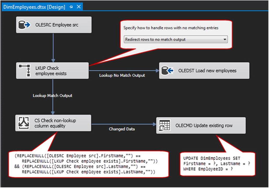
Figure 11-1. Incremental load using atomic SSIS components

Next, we’ll apply the Conditional Split transform to the matched rows. As shown in the snippet on the lower left of Figure 11-1, we’ll use a bit of the SSIS expression language to compare equivalent columns between source and destination. Any rows with an exact match will not go through any further processing (though you could send them to a Row Count transform if you want to capture the count of source rows with no action taken).

Finally, the rows that matched the business key but not the subsequent attribute values will be sent to the OLE DB Command transform. The code on the lower right in Figure 11-1 shows a snippet of the SQL code in which we perform a parameterized update of each row in the destination table. It is important to note that the OLE DB Command transform performs a row-by-row update against the target table. You can typically leverage this pattern as shown because most incremental operations are heavy on new rows and have far fewer updates than inserts. However, if a particular implementation requires the processing of a very large amount of data, or if your data exploration indicates that the number of updates is proportionally high, consider modifying this design pattern to send those rows meant for update out to a staging table where they can be more efficiently processed in a set-based operation.

Typical Uses

As mentioned previously, this incremental load design pattern is quite useful and mature. This pattern fits especially well when you are dealing with nonrelational source data, or when it’s not possible to stage incoming data before processing. This is often the go-to design for incremental loads, and it fits most of this type of scenario reasonably well.

Make sure you keep in mind that, because we’re performing the business key lookup and the column equivalency tests within SSIS, some resource costs are associated with getting the data into the SSIS memory space and then performing said operations against the data. Therefore, if a particular implementation involves a very large amount of data, and the source data is already in a SQL Server database (or could be staged there), another design pattern such as the T-SQL MERGE operation (to be covered shortly) might be a better option.

The following subsections describe components of the incremental load pattern and configuration options for each.

Lookup Caching Options

When performing lookup operations, you want to consider the many options available for managing lookup caching. Depending on the amount of data you’re dealing with, one of the following caching design patterns may help reduce performance bottlenecks.

Table Cache

A table cache for lookups is populated prior to executing a Data Flow task that requires the lookup operation. SSIS can create and drop the table as needed using Execute SQL tasks. It can be populated via the Execute SQL task or a Data Flow task. Most of the time, the data I need to build a table cache is local to the destination and contains data from the destination, so I often use T-SQL in an Execute SQL task to populate it.

You can maintaining the table cache by using truncate-and-load. However, for larger sets of lookup data, you may wish to consider maintaining the table cache using incremental load techniques. This may sound like overkill, but when you need to perform a lookup against a billion-row table (it happens, trust me), the incremental approach starts to make sense.

Cache Transformation and Cache Connection Manager

If you find you need to look up the same data in multiple Data Flow tasks, consider using the Cache transform along with the Cache connection manager. The Cache connection manager provides a memory-resident copy of the data supplied via the Cache transform. The cache is loaded prior to the first Data Flow task that will consume the lookup data, and the data can be consumed directly by a Lookup transform. Precaching data in this manner supports lookups, but it also provides a way to “mark” sets of rows for other considerations such as loading. Later in this chapter, we will explore late-arriving data and discuss patterns for managing it. One way to manage the scenario of data continuing to arrive after the load operation has started is to create a cache of primary and foreign keys that represent completed transactions, and then join to those keys in Data Flow tasks throughout the load process. Will you miss last-second data loading in this way? Yes, you will. But your data will contain complete transactions. One benefit of executing incremental loads with table caches is the ability to execute the load each month, week, evening, or every five minutes; only complete transactions that have arrived since the last load executed will be loaded.

If you find you need to use the same lookup data across many SSIS packages (or that the cache is larger than the amount of available server RAM), the Cache connection manager can persist its contents to disk. The Cache connection manager makes use of the new and improved RAW file format, a proprietary format for storing data directly from a Data Flow task to disk, completely bypassing connection managers. Reads and writes are very fast as a result, and the new format persists column names and data types.

Load Staging

Another pattern worth mentioning here is load staging. Consider the following scenario: a data warehouse destination table is large and grows often. Since the destination is used during the load window, dropping keys and indexes is not an option to improve load performance. All related data must become available in the data warehouse at roughly the same time to maintain source-transactional consistency. By nature, the data does not lend itself to partitioning. What to do?

Consider load staging, where all the data required to represent a source transaction is loaded into stage tables on the destination. Once these tables are populated, you can use Execute SQL tasks to insert the staged rows into the data warehouse destination table. If timed properly, you may be able to use a bulk insert to accomplish the load. Often, data loads between tables in the same SQL Server instance can be accomplished more efficiently using T-SQL rather than the buffered SSIS Data Flow task. How can you tell which will perform better? Test it!

The Slowly Changing Dimension Wizard

The Slowly Changing Dimension (SCD) Wizard is another veteran of the SSIS incremental load arsenal. As its name implies, it is designed specifically for managing SCD elements in a data warehouse. However, its use is certainly not limited to dimension processing.

The SCD Wizard has been a part of SSIS ever since the product’s introduction in 2005. At first glance, it is the natural choice for handling slowly changing dimension data in SSIS. This tool is built right into Integration Services, and it is designed specifically for the purpose of SCD processing.

The SCD Wizard is surfaced as a transformation in SSIS and is leveraged by connecting the output of a data source (the incoming data) to the input of the SCD transformation. Editing the SCD transformation will kick off the wizard, as shown in Figure 11-2.

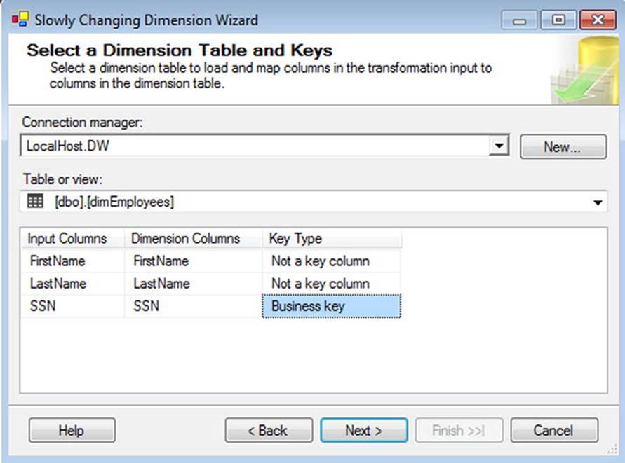
Figure 11-2. The SCD Wizard showing alignment of columns

From there, the wizard will guide you through the selection of the necessary elements of the SCD configuration, including the following:

· Which columns should be engaged as part of the SCD, along with the option to handle changes as simple updates (Type 1) or historical values (Type 2).

· How to identify current vs. expired rows, if any Type 2 columns are present; you can specify either a flag or a date span to indicate currency of SCD records.

· How to handle inferred members (discussed in more depth shortly).

When you’ve completed the SCD Wizard, several new elements are automatically added to the data flow. Figure 11-3 shows an example of the transforms and destinations added when using a combination of Type 1 and Type 2 fields, fixed-attribute (static) fields, and inferred member support. The SCD Wizard adds only those components pertinent to the design specified, so the final result may look a bit different than the example in this figure, depending on how the wizard is configured.

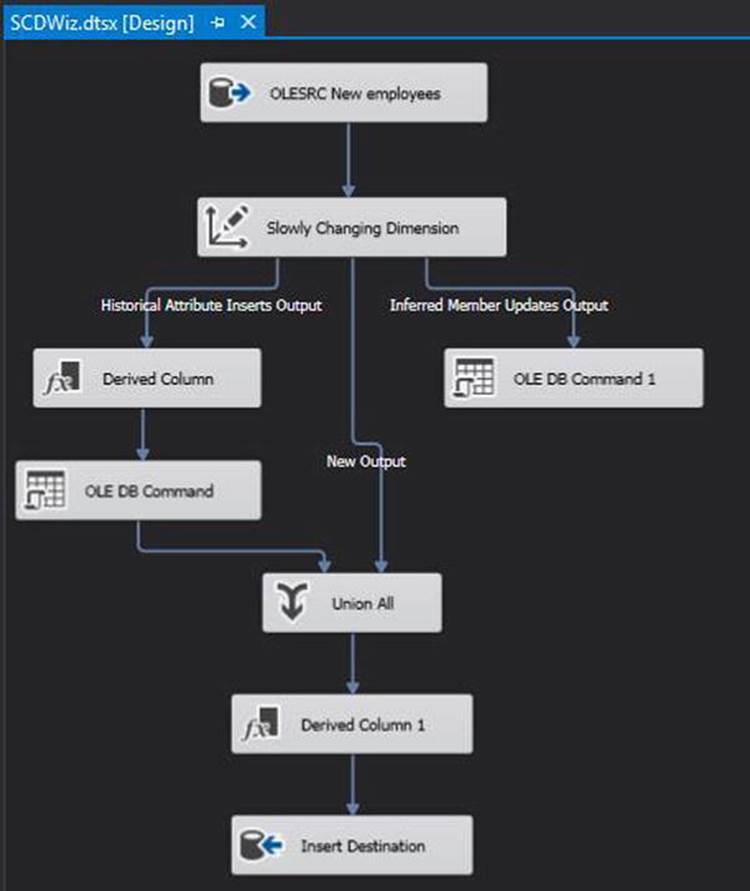
Figure 11-3. SCD Wizard output

Of all of the SCD design patterns, the SCD Wizard is arguably the easiest to use for simple SCD scenarios, and it offers the fastest turnaround at design time. For small, simple dimensions, the wizard can be an effective tool for managing changing data.

However, the SCD Wizard does have some significant drawbacks.

· Performance: The wizard performs reasonably well against small sets of data. However, because many of the operations are performed on a row-by-row basis, leveraging this transform against sizeable dimensions can cause a significant performance bottleneck. Some data warehouse architects have strong feelings against the SCD Wizard, and this is often the chief complaint.

· Destructive changes: As I mentioned, when you run the wizard, all of the required transforms and destinations are created automatically. Similarly, if you reconfigure the SCD transform (for example, changing a column type from a Type 1 to a Type 2 historical), the existing design elements are removed and added back to the data flow. As a result, any changes that you’ve made to that data path will be lost if you make a change to the SCD transform.

· No direct support for auditing: Although you can add your own auditing logic, it’s not a native function of this component. Further, because any changes to the SCD transformation will delete and re-create the relevant elements of the data flow, you’ll have to reconfigure that auditing logic if any changes are made to the SCD transform.

As a result of these shortcomings (especially the performance implications), the SCD Wizard doesn’t see a lot of action in the real world. I don’t want to beat up on this tool too much because it does have some usefulness, and I don’t necessarily recommend that you avoid it completely. However, like any specialty tool, it should be used only where appropriate. For small sets of SCD data that do not require complex logic or specialized logging, it can be the most effective option for SCD processing.

The MERGE Statement

Although technically not a function of SSIS, the MERGE statement has become such a large part of incremental data loads that any discussion focused on data warehousing design patterns would not be complete without this tool being covered.

A Little Background

Prior to version 2008, there were no native upserts (UPdate/inSERT) in Microsoft SQL Server. Any operation that blended updates and inserts required either the use of a cursor (which often performs very poorly) or two separate queries (usually resulting in duplicate logic and redundant effort). Other relational database products have had this capability for years—in fact, it has been present in Oracle since version 9i (around 2001). Naturally, SQL Server professionals were chomping at the bit for such capabilities.

Fortunately, they got their wish with the release of SQL Server 2008. That version featured the debut of the new MERGE statement as part of the T-SQL arsenal. MERGE allows three simultaneous operations (INSERT, UPDATE, and DELETE) against the target table.

The anatomy of a MERGE statement looks something like this:

1. Specify the source data.

2. Specify the target table.

3. Choose the columns on which to join the source and target data.

4. Indicate the column alignment between the two sets of data to be used for determining whether matched records are different in some way.

5. Define the logic for cases when the data is changed, or if it only exists in either the source or the destination.

The new MERGE capabilities are useful for DBAs and database developers alike. However, for data warehouse professionals, MERGE was a game changer in terms of managing SCD data. Not only did this new capability provide an easier way to perform upsert operations, but it also performed very well.

MERGE in Action

Since there are no native (read: graphical) hooks to the MERGE statement in Integration Services, the implementation of MERGE in an SSIS package is done through an Execute SQL task.

To explore this design pattern, let’s first examine the typical flow for using the T-SQL MERGE functionality within a data warehouse SSIS load package. Again, we’ll use the SCD scenario as a basis for exploration, but much of the same logic would apply to other uses of MERGE.

As part of an SCD MERGE upsert process, our SSIS package would contain tasks to perform the following functions:

1. Remove previously staged data from the staging table.

2. Load the staging table from the source system.

3. Clean up the staged data (if required).

4. Execute the MERGE statement to upsert the staged data to the dimension table.

5. Log the upsert operation (optional).

A typical control flow design pattern is shown in Figure 11-4.

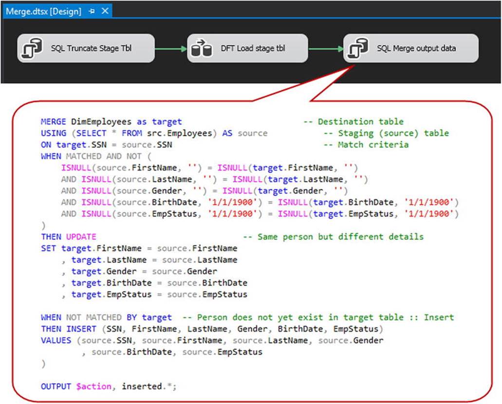
Figure 11-4. Using MERGE against a SCD table

Also note the large callout in Figure 11-4 with the T-SQL code used for the MERGE statement. In the interest of maintaining focus, I won’t try to provide comprehensive coverage of the MERGE statement here, but I’ll point out a couple of the high points:

· The ON clause (third line) indicates the field on which we join the source data with the destination data. Note that we can use multiple fields on which to align the two sets.

· The ten-line code block following WHEN MATCHED AND NOT... indicates which of the fields will be checked to see if the data in the destination table differs from the source data. In this case, we’re checking ten different fields, and we’ll process an update to the destination if any of those fields is different between the source and destination. Also note the liberal use of the ISNULL() function against the destination table. This is recommended to ensure that rows in the destination table containing NULL values are not inadvertently skipped during the MERGE.

· In the code block immediately following, we update rows in the target table that have a valid match against the source but have one or more values that differ between the two.

· In the code block beginning with WHEN NOT MATCHED BY target..., any source rows not matched to the specified key column(s) of an existing dimension record are written as new rows to that dimension table.

· Finally, we use the OUTPUT clause to select the action description and insert data. We can use the output of this to write to our auditing table (more on that momentarily).

You’ll notice that we’re handling this dimension processing as a Type 1 dimension, in which we intentionally overwrite the previous values and do not maintain a historical record of past values. It is possible to use the MERGE command to process Type 2 dimensions that retain historical values, or even those with a mixture of Type 1 and Type 2 attributes. In the interest of brevity, I won’t try to cover the various other uses of MERGE as it applies to slowly changing dimensions, but I think you’ll find that it’s flexible enough to handle most Type 1 and Type 2 dimensions.

It is also worth noting that you can also use the MERGE statement to delete data in addition to performing inserts and updates. It’s not as common to delete data in data warehouse environments as it is in other settings, but you may occasionally find it necessary to delete data from the target table.

Auditing with MERGE

As with other data warehouse operations, it’s considered a best practice to audit, at a minimum, the row counts of dimensional data that is added, deleted, or changed. This is especially true for MERGE operations. Because multiple operations can occur in the same statement, it’s important to be able to track those operations to assist with troubleshooting, even if comprehensive auditing is not used in a given operation.

The MERGE statement does have a provision for auditing the various data operations. As shown in the example in Figure 11-4, we can use the OUTPUT clause to select out of the MERGE statement the INSERT, UPDATE, or DELETE operations. This example shows a scenario where the data changes would be selected as a result set from the query, which could subsequently be captured into a package variable in SSIS and processed from there. Alternatively, you could modify the OUTPUT clause to insert data directly into an audit table without returning a result set to SSIS.

Change Data Capture (CDC)

Along with the MERGE capability, another significant incremental load feature first surfaced in SQL Server 2008: change data capture (CDC). CDC is a feature of the database engine that allows the collection of data changes to monitored tables.

Without jumping too far off track, here’s just a bit about how CDC works. CDC is a supply-side incremental load tool that is enabled first at the database level and then implemented on a table-by-table basis via capture instances. Once CDC is enabled for a table, the database engine uses the transaction log to track all DML operations (INSERTs, UPDATEs, and DELETEs), logging each change to the change table for each monitored table. The change table contains not only the fact that there was a change to the data, but it also maintains the history of those changes. Downstream processes can then consume just the changes (rather than the entire set of data) and process the, INSERTs, UPDATEs, and DELETEs in any dependent systems.

CDC in Integration Services

SSIS can consume CDC data in a couple of different ways. First, using common native SSIS components, you can access the change table to capture the data changes. You can keeping track of which changes have been processed by SSIS by capturing and storing the log sequence number (LSN) by using a set of system stored procedures created when CDC is enabled.

The manual methods are still valid; however, new to SSIS in SQL Server 2012 is an entirely new set of tools for interfacing with CDC data. Integration Services now comes packaged with a new task and two new components that help to streamline the processing of CDC data:

· CDC Control task: This task is used for managing the metadata around CDC loads. Using the CDC Control task, you can track the start and end points of the initial (historical) load, as well as retrieve and store the processing range for an incremental load.

· CDC Source: The CDC Source is used to retrieve data from the CDC change table. It receives the CDC state information from the CDC Control task by way of an SSIS variable, and it will selectively retrieve the changed data using that marker.

· CDC Splitter: The CDC Splitter is a transform that will branch the changed data out into its various operations. Effectively a specialized Conditional Split transform, it will use the CDC information received from the CDC Source and send the rows to the Insert, Update, Delete, or Error path accordingly.

For the purposes of reviewing CDC capabilities as part of an SSIS incremental load strategy, we’ll stick with the new task and components present in SSIS 2012. In systems using SQL Server 2008, know that you can meet the same objectives by employing the manual extraction and LSN tracking briefly described previously.

Change Detection in General

Detecting changes in data is a subscience of data integration. Much has been written on the topic from sources too numerous to list. Although CDC provides handy change detection in SQL Server, it was possible (and necessary!) to achieve change detection before the advent of CDC. It is important to note that CDC is not available in all editions of SQL Server; it is also not available in other relational database engines.

Checksum-Based Detection

One early pattern for change detection was using the Transact-SQL Checksum function. Checksum accepts a string as an argument and generates a numeric hash value. But Checksum performance has proven less than ideal, generating the same number for different string values. Steve Jones blogged about this behavior in a post entitled “SQL Server Encryption—Hashing Collisions” (www.sqlservercentral.com/blogs/steve_jones/2009/06/01/sql-server-encryption-hashing-collisions/). Michael Coles provided rich evidence to support Steve’s claims in the post’s comments (www.sqlservercentral.com/blogs/steve_jones/2009/06/01/sql-server-encryption-hashing-collisions/#comments). In short, the odds of collision with Checksums are substantial, and you should not use the Checksum function for change detection.

So, what can you use?

Detection via Hashbytes

One good alternative to the Checksum function is the Hashbytes function. Like Checksum, Hashbytes provides value hashing for a string value or variable. Checksum returns an integer value; Hashbytes returns a binary value. Checksum uses an internal algorithm to calculate the hash; Hashbytes uses standard encryption algorithms. The sheer number of values available to each function is one reason Hashbytes is a better choice. Checksum’s int data type can return +/-231 values, whereas Hashbytes can return +/-2127 values for MD2, MD4, and MD5 algorithms and +/-2159 values for SHA and SHA1 algorithms.

Brute Force Detection

Believe it or not, a “brute force” value comparison between sources and destinations remains a viable option for change detection. How does it work? You acquire the destination values by way of either a second Source component or a Lookup transform in the SSIS Data Flow task. You match the rows in the source and destination by using an alternate (or business) key—a value or combination of values that uniquely identifies the row in both source and destination—and then compare the non-key column values in the source row to the non-key values in the destination row.

Remember, you are attempting to isolate changes. It is assumed that you have separated the new rows—data that exists in the source and not in the destination—and perhaps you have even detected deleted rows that exist in the destination but are no longer found in the source. Changed and unchanged rows remain. Unchanged rows are just that: the alternate keys align, as does every other value in each source and destination column. Changed rows, however, have identical alternate keys and one or more differences in the source and destination columns. Comparing the column values and accounting for the possibility of NULLs remains an option.

Historical Load

There should be a separate process to populate the historical data for each of the tracked CDC tables. This historical load is designed to be executed just once, and it would load data to the destination system from as far back as is required. As shown in Figure 11-5, two CDC Control tasks are required. The first one (configured as shown in the callout) is used to set the beginning boundary of the data capture. With this information, the CDC Control task writes the CDC state to the specified state table. The second CDC Control task marks the end point of the initial load, updating the state table so the appropriate starting point will be used on subsequent incremental loads. Between these two tasks sits the data flow, which facilitates the historical load of the target table.

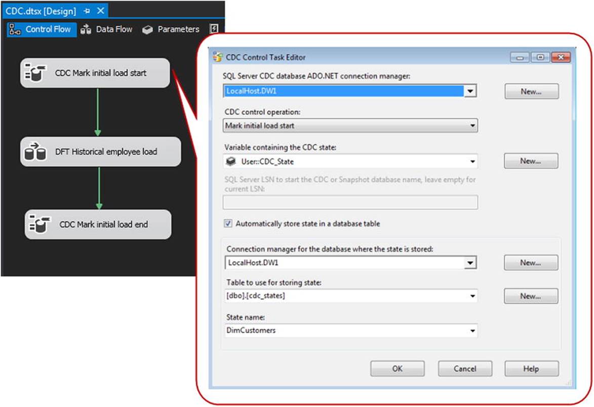
Figure 11-5. CDC Control task for an initial historical load

Incremental Load

Because of the inherent differences between historical loads and incremental loads, it’s almost always preferable to create separate packages (or package groups) for each of these. Although there are similarities, there are enough differences to justify separating the logic into different sandboxes.

For the control flow elements of the historical load, this incremental load pattern will also use two CDC Control tasks with a data flow between them. We’ll need to slightly change the configuration of these tasks so that we retrieve and then update the current processing range of the CDC operation. As shown in Figure 11-6, we’ll set the operation for the first of these as Get Processing Range, which would be followed by Update Processing Range after the incremental load is complete.

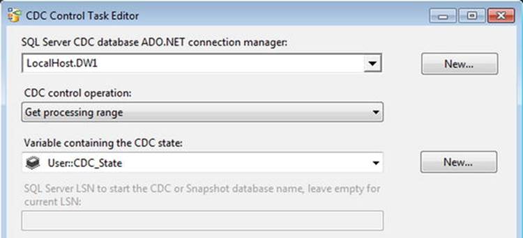
Figure 11-6. Get processing range for CDC incremental load

Note The CDC Control task is a versatile tool that includes several processing modes to handle various CDC phases, including dealing with a snapshot database or quiescence database as a source. A complete listing of the processing modes can be found here:http://msdn.microsoft.com/en-us/library/hh231079.aspx.

Within the data flow, the CDC Source should be set with the table from which to capture, the capture instance, and the processing mode. In this case, we’re going to use “Net” to retrieve the net changes to the CDC table. See Figure 11-7.

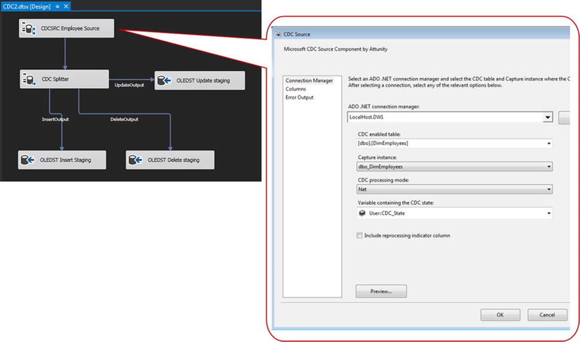
Figure 11-7. CDC Source

The CDC Splitter breaks apart the data stream and sends rows out to the insert, update, and delete outputs. From there, we’ll write the update and delete rows to a staging table so we can process those as high-performance, set-based operations. The insert records can go directly into the output table.

It’s worth mentioning here that several CDC processing modes are available through the CDC Source component. The example in Figure 11-7 illustrated the use of the Net setting, which is the most common mode in most data warehouse scenarios. However, depending on the ETL requirements and source system design, you may opt for one of the other processing modes, as follows:

· All: Lists each change in the source, not just the Net result

· All with Old Values: Includes each change plus the old values for updated records

· Net with Update Mask: Is for monitoring changes to a specific column in the monitored table

· Net with Merge: Is similar to Net, but the output is optimized for consumption by the T-SQL MERGE statement

Typical Uses

CDC represents a shift in the incremental load methodology. The other methods described here apply a downstream approach to incremental loading, with a minimally restrictive extraction from the source and a decision point late in the ETL flow. CDC, on the other hand, processes the change logic further upstream, which can help lighten the load on SSIS and other moving parts in the ETL.

If CDC is in place (or could be implemented) in a source system, it’s certainly worth considering using this design pattern to process incremental loads. It can perform well, can reduce network loads due to processing fewer rows from the source, and requires fewer resources on the ETL side. It’s not appropriate for every situation, but CDC can be an excellent way to manage incremental loads in SQL Server Integration Services.

Keep in mind that the use of CDC as a design pattern isn’t strictly limited to Microsoft SQL Server databases. CDC may also be leveraged against CDC-enabled Oracle database servers.

Data Errors

Henry Wadsworth Longfellow once wrote, “Into each life some rain must fall.” The world of ETL is no different, except that rain comes in the form of errors, often as a result of missing or invalid data. We don’t always know when they’re going to occur. However, given enough time, something is going to go wrong: late-arriving dimension members, packages executed out of order, or just plain old bad data. The good news is that there are data warehousing design patterns that can help mitigate the risk of data anomalies that interrupt the execution of Integration Services packages.

To address patterns of handling missing data, we’re going to concentrate mostly on missing dimension members, as this is the most frequent cause of such errors. However, you can extend some of the same patterns to other elements that are part of or peripheral to data warehousing.

Simple Errors

The vast majority of errors can and should be handled inline, or simply prevented before they occur. Consider the common case of data truncation: you have a character type field that’s expected to contain no more than 50 characters, so you set the data length accordingly. Months later, you get a late-night phone call (most likely when you’re on vacation or when you’re out at a karaoke bar with your fellow ETL professionals) informing you that the SSIS package has failed because of a truncation error. Yep, the party’s over.

We’ve all been bitten before by the truncation bug or one of its cousins—the invalid data type error, the unexpected NULL/blank value error, or the out-of-range error. In many cases, however, these types of errors can be handled through defensive ETL strategies. By using tasks and components that detect and subsequently correct or redirect nonconforming rows, we can handle minor data errors such as this without bubbling up a failure that stops the rest of the ETL from processing.

Missing Data

With respect to data warehousing, a more common example of handling errors inline is the case of late-arriving dimension data. As shown in Figure 11-8, the typical pattern is to load the dimensions first, followed by a load of the fact tables. This helps to ensure that the fact records will find a valid dimension key when the former is loaded to the data warehouse.

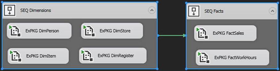
Figure 11-8. Typical data warehouse methodology of loading dimensions, then facts

However, this pattern breaks down when you attempt to process fact records that reference dimension data that does not yet exist in the data warehouse. Consider the case of holiday retail sales: because things happen so quickly at the retail level during the end-of-year holiday season, it’s not uncommon for last-minute items to appear at a store’s dock with little or no advance notice. Large companies (retailers included) often have multiple systems used for different purposes that may or may not be in sync, so a last-minute item entered in the point-of-sale (POS) system may not yet be loaded in the sales forecasting system. As a result, an attempt to load a data warehouse with both POS and forecasting data may not fit this model because we would have fact data from the sales system that do not yet have the required dimension rows from the forecasting system.

At this point, if the decision is made to handle this issue inline, there are a few different methodogies we can use. These are described next.

Use the Unknown Member

The fastest and simplest pattern to address the issue of missing dimension members is to push fact records with missing dimension data into the fact table while marking that dimension value as unknown. In this case, the fact records in question would be immediately available in the data warehouse; however, all of the unknowns would, by default, be grouped together for analytical purposes. This pattern generally works best when the fact record alone does not contain the required information to create a unique new dimension record.

This design pattern is fleshed out in Figure 11-9. Using the No Match output of the Lookup transform, we’re sending the fact records not matched to an existing [Item] dimension member to an instance of the Derived Column transform, which sets the value of the missing dimension record to the unknown member for that dimension (in most cases, represented by a key value of –1). The matched and unmatched records are then brought back together using the Union All transform.

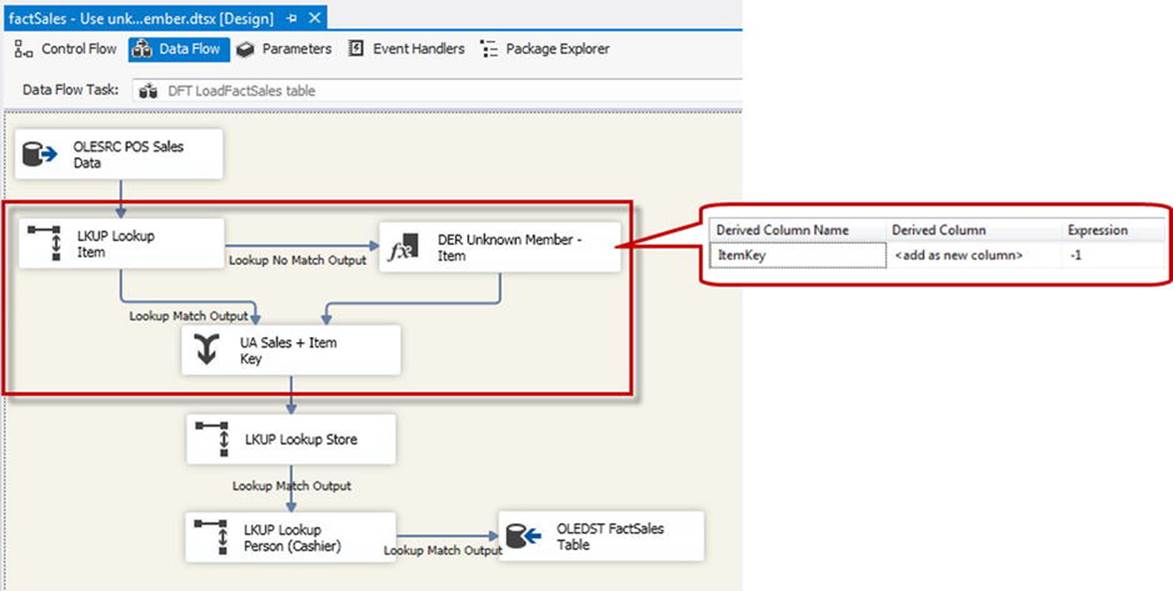
Figure 11-9. Using Unknown Member for missing dimension member

It is important to note that this design pattern should also include a supplemental process (possibly consisting of just a simple SQL statement) to periodically attempt to match these modified facts with their proper dimension records. This follow-up step is required to prevent the fact data in question from being permanently linked to the unknown member for that dimension.

Add the Missing Dimension Member

Using this design pattern, you can add missing dimension records on the fly as part of the fact package using as much dimension data as is provided by the fact data. In this scenario, the fact records are immediately available in the data warehouse, just like they were for the previous design pattern, but this methodology has the added benefit of matching the fact record to its proper dimension member. In most cases, this allows you to immediately associate the correct dimension data rather than group the unmatched data into the unknown member bucket.

Like the previous pattern, this method does come with a couple of caveats. First of all, the fact record must contain all of the information to 1) satisfy the table constraints (such as NOT NULL restrictions) on the dimension table, and 2) create a uniquely identifiable dimension row using the business key column(s). Also, since we’re deriving the newly added dimension member from the incoming fact records, in most cases,mit can be reasonably assumed that the incoming fact data will not completely describe the dimension member. For that reason, you should also complement this design pattern with a process that attempts to fill in the missing dimension elements (which may already be addressed as part of a comprehensive slowly changing dimension strategy).

As shown in Figure 11-10, here we use a methodology similar to the previous example. However, instead of simply assigning the value of the unknown member using the Derived Column transform, we leverage an instance of the OLE DB Command transform to insert the data for the missing dimension record in the fact table into the dimension table. The SQL statement is shown in the callout, and in the properties of the OLE DB command, we map the placeholders (indicated by question marks) to the appropriate values from the fact record.

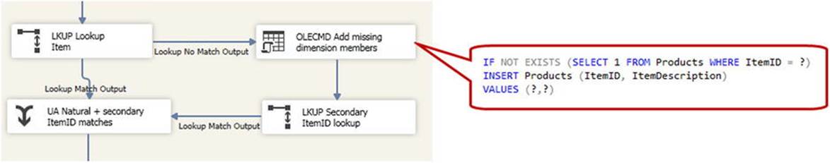
Figure 11-10. Adding the missing dimension member

After adding the missing member, we send those rows to a secondary ItemID lookup, which will attempt (successfully, unless something goes terribly wrong) to match the previously unmatched data with the newly added dimension records in the DimItem table. It is important that you remember to set the cache mode to either Partial Cache or No Cache when using a secondary lookup in this manner. The default lookup cache setting (Full Cache) will buffer the contents of the Item dimension table before the data flow is initiated, and as a result, none of the rows added during package execution would be present in this secondary lookup. To prevent all of these redirected fact rows from failing the secondary Item dimension lookup, use one of the non-default cache methods to force the package to perform an on-demand lookup to include the newly added dimension values.

Regarding the secondary lookup transformation methodology, you might wonder if the second lookup is even necessary. After all, if we perform the insert in the previous step (OLE DB command), couldn’t we just collect the new Item dimension key value (a SQL Server table identity value, in most cases) using that SQL statement? The answer is a qualified yes, and in my experience, that is the simpler of the two options. However, I’ve also found that some ETL situations—in particular, the introduction of parallel processes performing the same on-the-fly addition of dimension members—can cloud the issue of collecting the identity value of the most recently inserted record. From that perspective, I lean toward using the secondary lookup in cases such as this.

Triage the Lookup Failures

For missing dimension records, the most common approaches typically involve one of the preceding. However, on occasion it will be necessary to delay the processing of fact records that do not match an existing dimension record. In cases such as this, you’ll need to create a triage table that will store the interim records until they can be successfully matched to the proper dimension.

As shown in Figure 11-11, we’re adding a couple of additional components to the ETL pipeline for this design pattern. At the outset, we need to use two separate sources of data: one to bring in the new data from the source system, and the other for reintroducing previously triaged data into the pipeline. Further into the data flow, the example shows that we are redirecting the unmatched fact records to another table rather than trying to fix the data inline.

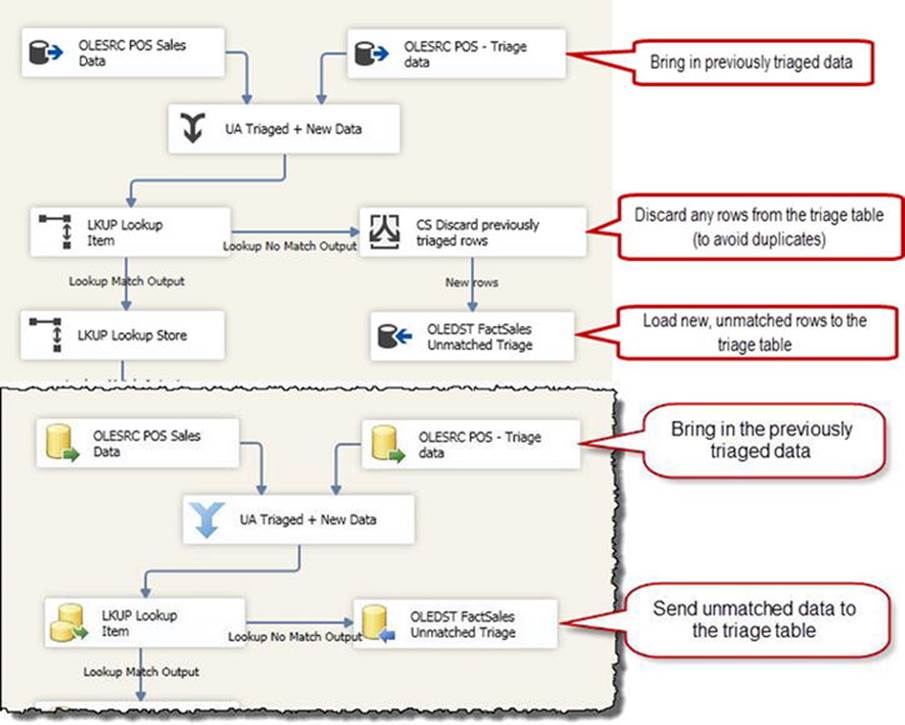
Figure 11-11. Use a triage table to store unmatched fact data

As an aside, this pattern could be modified to support manual intervention for correcting failed lookups as well. If the business and technical requirements are such that the unmatched fact data must be reviewed and corrected by hand (as opposed to a systematic cleanup), you could eliminate the triage source so that the triage data is not reintroduced into the data flow.

Coding to Allow Errors

Although it may sound like an oxymoron, it’s actually a common practice to code for known errors. In my experience, the nature of most ETL errors dictates that the package execution can continue, and any errors or anomalies that cannot be addressed inline are triaged, as shown in the previous example (with the appropriate notification to the person responsible, if manual intervention is required), for later resolution. However, there are situations where the data warehouse ETL process should be designed to fail if error conditions arise.

Consider the case of financial data. Institutions that store or process financial data are subject to frequent and comprehensive audits, and if inconsistent data appeared in a governmental review of the data, it could spell disaster for the organization and its officers. Even though a data warehouse may not be subject to the same to-the-penny auditing scrutiny as OLTP systems, there is still an expectation of consistency when matters of money and governmental regulation are involved. In the case of a data warehouse load where nonconforming data is encountered, quite possibly the best thing to occur is that the package fails gracefully, rolling back any changes made as part of the load.

Fail Package on Error

Extending the financial data example mentioned previously, let’s examine the design pattern to facilitate a failure in the event of a lookup error. In reality, this is the default behavior. As shown in Figure 11-12, we use the default setting of Fail Component on the lookup components, which stops the execution of the package if a row is encountered that cannot be matched to either the GL Account or GL Subaccount lookup.

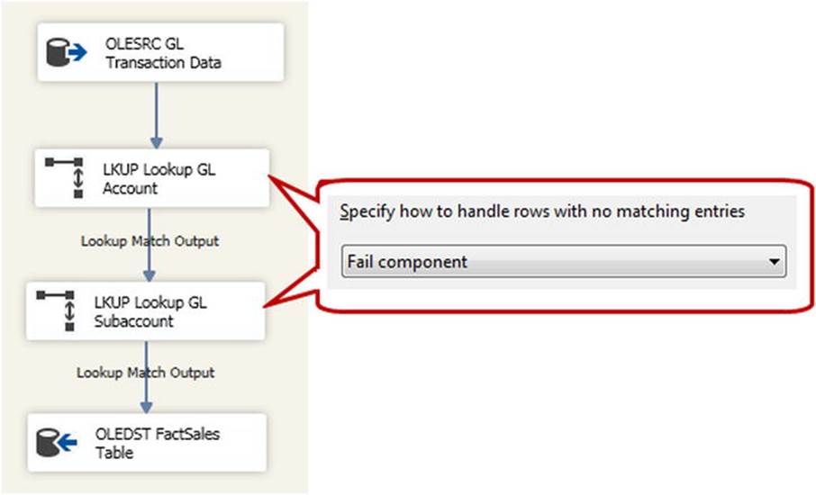
Figure 11-12. Allow the package to fail upon error

It’s worth noting here that to properly use this design pattern, you must include some logic to roll back changes due to a partial load. If you encounter a fact row that does not match one of the lookup components, the package will still fail; however, you may commit rows preceding the errored row that have already been sent to the destination to that table before the failure and can cause all the data to be in an inconsistent state.

There are several ways to accomplish this rollback 'margin-top:6.0pt;margin-right:29.0pt;margin-bottom: 6.0pt;margin-left:65.0pt;text-indent:-18.0pt;line-height:normal'>· SSIS transactions: Integration Services natively has the ability to wrap tasks and containers into transactions and, in theory, will reverse any durable changes to the relational database in the event of an error in the scope of that transaction. In practice, however, I’ve found that using the SSIS transaction functionality can be challenging even on a good day. Leveraging transactions directly in SSIS requires a lot of things to align at once: all involved systems must support DTC transactions, the DTC service must be running and accessible at each of those endpoints, and all relevant tasks and connections in SSIS must support transactions.

· Explicit SQL transactions: This method involves manually creating a transaction in SSIS by executing the T-SQL command to engage a relational transaction on the database engine. Using this method, you essentially create your own transaction container by explicitly declaring the initialization and COMMIT point (or ROLLBACK, in the event of an error) using the Execute SQL task. On the database connection, you’ll need to set the RetainSameConnection property to True to ensure that all operations reuse the same connection and, by extension, the same transaction. Although this method does require some additional work, it’s the more straightforward and reliable of the two transactional methods of strategic rollback.

· Explicit cleanup: This design pattern involves creating your own environment-specific cleanup routines to reverse the changes due to a failed partial load, and it typically does not engage database transactions for rollback purposes. This method requires the most effort in terms of development and maintenance, but it also allows you the greatest amount of flexibility if you need to selectively undo changes made during a failed package execution.

Unhandled Errors

I’m certain that the gentleman who came up with Murphy’s Law was working as a data warehouse ETL developer. Dealing with data from disparate systems is often an ugly process! Although we can defensively code around many common issues, eventually some data anomaly will introduce unexpected errors.

To make sure that any error or other data anomaly does not cause the ETL process to abruptly terminate, it’s advisable to build in some safety nets to handle any unexpected errors.

Data Warehouse ETL Workflow

Most of what has been covered in this chapter so far has been core concepts about the loading of data warehouses. I’d like to briefly change gears and touch on the topic of SSIS package design with respect to workflow. Data warehouse ETL systems tend to have a lot of moving parts, and the workload to develop those pieces is often distributed to multiple developers. Owing to a few lessons learned the hard way, I’ve developed a workflow design pattern of package atomicity.

Dividing Up the Work

I’ve told this story in a couple of presentations I’ve done, and it continues to be amusing (to me, anyway) to think about ever having done things this way. The first production SSIS package of any significance that I deployed was created to move a large amount of data from multiple legacy systems into a new SQL Server database. It started off rather innocently; it initially appeared that the ETL logic would be much simpler than what it eventually became, so I wrapped everything into a single package.

In the end, the resulting SSIS package was enormous. There were 30, maybe 40, different data flows (some with multiple sources/destinations and complex transformation logic) and dozens of other helper tasks intermingled. The resulting .dtsx file size was about 5MB just for the XML metadata! Needless to say, every time I opened this package in Visual Studio, it would take several minutes to run through all of the validation steps.

This extremely large SSIS package worked fine, and technically there was nothing wrong with the design. Its sheer size did bring to light some challenges that are present in working with large, do-everything packages, and as a result of that experience, I reengineered my methodology for atomic package design.

One Package = One Unit of Work

With respect to data warehouse ETL, I’ve found that the best solution in most cases is to break apart logical units of work into separate packages in which each package does just one thing. By splitting up the workload, you can avoid a number of potential snags and increase your productivity as an ETL developer. Some of the considerations for smaller SSIS packages include the following:

· Less time spent waiting on design-time validation: SQL Server Data Tools has a rich interface that provides, among other things, a near real-time evaluation of potential metadata problems in the SSDT designer. If, for example, a table that is accessed by the SSIS package is changed, the developer will be presented with a warning (or an error, if applicable) in SSDT indicating that metadata accessed by the package has changed. This constant metadata validation is beneficial in that it can help to identify potential problems before they are pushed out for testing. There’s also a performance cost associated with this. The length of time required for validation increases as the size of the package increases, so naturally keeping the packages as small as practical will cut down on the amount of time you’re drumming your fingers on your desk waiting for validation to complete.

· Easier testing and deployment: A single package that loads, say, ten dimensions has a lot of moving parts. When you are developing each of the dimensions within the package, there is no easy way to test just one element of the package (apart from manually running it in the SSDT designer, which isn’t a completely realistic test for a package that will eventually be deployed to the server). The only realistic test for such a package is to test the entire package as a server-based execution, which may be overkill if you’re only interested in one or two changed properties. Further, it’s not uncommon for organizations with formal software testing and promotion procedures to require that the entire thing be retested, not just the new or changed elements. By breaking up operations into smaller units, you can usually make testing and deployment less of a burden because you are only operating on one component at a time.

· Distributed development: If you work in an environment where you are the only person developing SSIS packages, this is less of a concern. However, if your shop has multiple ETL developers, those do-everything packages are quite inconvenient. Although it’s much easier in SQL Server 2012 than in previous releases to compare differences between versions of the same package file, it’s still a mostly manual process. By segmenting the workload into multiple packages, it’s much easier to farm out development tasks to multiple people without having to reconcile multiple versions of the same package.

· Reusability: It’s not uncommon for the same logic to be used more than once in the same ETL execution, or for that same logic to be shared among multiple ETL processes. When you encapsulate these logical units of work into their own packages, it’s much easier to share that logic and avoid duplicate development.

It is possible to go overboard here. For example, if, during the course of the ETL execution, you need to drop or disable indexes on 20 tables, you probably don’t need to create a package for each index! Break operations up into individual packages, but be realistic about what constitutes a logical unit of work.

These aren’t hard and fast rules, but with respect to breaking up ETL work into packages, here are a few design patterns that I’ve found work well when populating a data warehouse:

· Each dimension has a separate package.

· Each fact table has a separate package.

· Staging operations (if used) each have their own package.

· Functional operations unrelated to data movement (for example, dropping or disabling indexes on tables before loading them with data) are separated as well. You can group some of these operations together in common packages where appropriate; for example, if you truncate tables and drop indexes in a staging database, those operations typically reside in the same package.

Further, it’s often a good practice to isolate in separate packages any ETL logic that is significantly different in terms of scope or breadth of data. For example, a historical ETL process that retrieves a large chunk of old data will likely have different performance expectations, error-handling rules, and so on than a more frequently executed package that collects just the most recent incremental data. As such, by creating a separate package structure to address those larger sets of data, you help avoid the issue of trying to force a single package to handle these disparate scenarios.

Conclusion

SQL Server Integration Services isn’t just another ETL tool. At its root, it is ideally suited for the unique challenges of data warehouse ETL. This chapter has shown some specific methodologies for how to leverage SSIS against common and realistic DW challenges.