Functional Thinking (2014)
Chapter 3. Cede
Confession: I never want to work in a non-garbage-collected language again. I paid my dues in languages like C++ for too many years, and I don’t want to surrender the conveniences of modern languages. That’s the story of how software development progresses. We build layers of abstraction to handle (and hide) mundane details. As the capabilities of computers have grown, we’ve offloaded more tasks to languages and runtimes. Developers used to shun interpreted languages as too slow, but they are now commonplace. Many of the features of functional languages were prohibitively slow a decade ago but make perfect sense now because they optimize developer time and effort.
One of the values of functional thinking is the ability to cede control of low-level details (such as garbage collection) to the runtime, eliminating a swath of bugs you must chase. While many developers are accustomed to blissful ignorance for bedrock abstractions such as memory, they are less accustomed to similar abstractions appearing at a higher level. Yet these higher-level abstractions serve the same purpose: handling the mundane details of machinery while freeing developers to work on unique aspects of their problems.
In this chapter, I show five ways developers in functional languages can cede control to the language or runtime, freeing themselves to work on more relevant problems.
Iteration to Higher-Order Functions
I already illustrated the first example of surrendering control in Example 2-3, replacing iteration with functions such as map. What’s ceded here is clear: if you can express which operation you want to perform in a higher-order function, the language will apply it efficiently, including the ability to parallelize the operation with the addition of the par modifier.
Multithreaded code represents some of the most difficult and error-prone code to write and debug. Offloading the headache of thread management to a helper allows the developer to care less about the underlying plumbing.
That doesn’t mean that developers should cede all responsibility for understanding what happens in lower-level abstractions. In many cases, you still must understand the implications of using abstractions such as Stream. For example, many developers were surprised that they still had to understand details of the Fork/Join library to achieve high performance, even with the new Stream API in Java 8. Once you understand it, however, you can apply that power in a more succinct way.
NOTE
Always understand one level below your normal abstraction layer.
Programmers rely on abstraction layers to be effective: no one programs a computer by manipulating bits of rust on hard drives using just 0 and 1. Abstractions hide messy details from us, but they sometimes hide important considerations as well. I discuss this issue in more depth inChapter 8.
Closures
All functional languages include closures, yet this language feature is often discussed in almost mystical terms. A closure is a function that carries an implicit binding to all the variables referenced within it. In other words, the function (or method) encloses a context around the things it references.
Here is a simple example, written in Groovy, of creating a closure block with a binding, shown in Example 3-1.
Example 3-1. Simple closure binding in Groovy
classEmployee {
def name, salary
}
def paidMore(amount) {
return {Employee e -> e.salary > amount}
}
isHighPaid = paidMore(100000)
In Example 3-1, I define a simple Employee class with two fields. Then, I define a paidMore function that accepts a parameter amount. The return of this function is a code block, or closure, accepting an Employee instance. The type declaration is optional but serves as useful documentation in this case. I can assign this code block to the name isHighPaid, supplying the parameter value of 100,000. When I make this assignment, I bind the value of 100,000 to this code block forever. Thus, when I evaluate employees via this code block, it will opine about their salaries by using the permanently bound value, as shown in Example 3-2.
Example 3-2. Executing the closure block
def Smithers = new Employee(name:"Fred", salary:120000)
def Homer = new Employee(name:"Homer", salary:80000)
println isHighPaid(Smithers)
println isHighPaid(Homer)
// true, false
In Example 3-2, I create a couple of employees and determine if their salaries meet the criterion. When a closure is created, it creates an enclosure around the variables referenced within the scope of the code block (thus the name closure). Each instance of the closure block has unique values, even for private variables. For example, I can create another instance of my paidMore closure with another binding(and therefore another assignment), as shown in Example 3-3.
Example 3-3. Another closure binding
isHigherPaid = paidMore(200000)
println isHigherPaid(Smithers)
println isHigherPaid(Homer)
def Burns = new Employee(name:"Monty", salary:1000000)
println isHigherPaid(Burns)
// false, false, true
Closures are used quite often as a portable execution mechanism in functional languages and frameworks, passed to higher-order functions such as map() as the transformation code. Functional Java uses anonymous inner classes to mimic some of “real” closure behavior, but they can’t go all the way because Java before version 8 didn’t include closures. But what does that mean?
Example 3-4 shows an example of what makes closures so special.
Example 3-4. How closures work (in Groovy)
def Closure makeCounter() {
def local_variable = 0
return { return local_variable += 1 } // ![]()
}
c1 = makeCounter() // ![]()
c1() // ![]()
c1()
c1()
c2 = makeCounter() // ![]()
println "C1 = ${c1()}, C2 = ${c2()}"
// output: C1 = 4, C2 = 1 // ![]()
![]()
The return value of the function is a code block, not a value.
![]()
c1 now points to an instance of the code block.
![]()
Calling c1 increments the internal variable; if I evaluated this expression, it would yield 1.
![]()
c2 now points to a new, unique instance of makeCounter().
![]()
Each instance has a unique instance of the internal state held in local_variable.
The makeCounter() function first defines a local variable with an appropriate name, then returns a code block that uses that variable. Notice that the return type for the makeCounter() function is Closure, not a value. That code block does nothing but increment the value of the local variable and return it. I’ve placed explicit return calls in this code, both of which are optional in Groovy, but the code is even more cryptic without them.
To exercise the makeCounter() function, I assign the code block to a variable named c1, then call it three times. I’m using Groovy’s syntactic sugar to execute a code block (rather than the more verboase c1.call()), which is to place a set of parentheses adjacent to the code block’s variable. Next, I call makeCounter() again, assigning a new instance of the code block to a variable c2. Last, I execute c1 again along with c2. Note that each of the code blocks has kept track of a separate instance of local_variable. The origin of the word closure hints to its operation via creating an enclosing context. Even though a local variable is defined within the function, the code block is bound to that variable because it references it, meaning that it must keep track of it while the code block instance is alive.
From an implementation standpoint, the closure instance holds onto an encapsulated copy of whatever is in scope when the closure is created, such as local_variable in Example 3-4. When the closure block is garbage collected, all the references it owns are reclaimed as well.
It’s a bad idea to create a closure just so that you can manipulate its interior state—it’s done here to illustrate the inner workings of closure bindings. Binding constant or immutable values (as shown in Example 3-1) is more common.
The closest you could come to the same behavior in Java prior to Java 8, or in fact any language that has functions but not closures, appears in Example 3-5.
Example 3-5. makeCounter() in Java
classCounter {
publicint varField;
Counter(int var) {
varField = var;
}
publicstatic Counter makeCounter() {
returnnew Counter(0);
}
publicint execute() {
return ++varField;
}
}
Several variants of the Counter class are possible (creating anonymous versions, using generics, etc.), but you’re still stuck with managing the state yourself. This illustrates why the use of closures exemplifies functional thinking: allow the runtime to manage state. Rather than forcing yourself to handle field creation and babying state (including the horrifying prospect of using your code in a multithreaded environment), cede that control and let the language or framework invisibly manage that state for you.
NOTE
Let the language manage state.
Closures are also an excellent example of deferred execution. By binding code to a closure block, you can wait until later to execute the block. This turns out to be useful in many scenarios. For example, the correct variables or functions might not be in scope at definition time but are at execution time. By wrapping the execution context in a closure, you can wait until the proper time to execute it.
Imperative languages use state to model programming, exemplified by parameter passing. Closures allow us to model behavior by encapsulating both code and context into a single construct, the closure, that can be passed around like traditional data structures and executed at exactly the correct time and place.
NOTE
Capture the context, not the state.
Currying and Partial Application
Currying and partial application are language techniques derived from mathematics (based on work by twentieth-century mathematician Haskell Curry and others). These techniques are present in various types of languages and are omnipresent in functional languages in one form or another. Both currying and partial application give you the ability to manipulate the number of arguments to functions or methods, typically by supplying one or more default values for some arguments (known as fixing arguments). Most functional languages include currying and partial application, but they implement them in different ways.
Definitions and Distinctions
To the casual observer, currying and partial application appear to have the same effect. With both, you can create a version of a function with presupplied values for some of the arguments:
§ Currying describes the conversion of a multiargument function into a chain of single-argument functions. It describes the transformation process, not the invocation of the converted function. The caller can decide how many arguments to apply, thereby creating a derived function with that smaller number of arguments.
§ Partial application describes the conversion of a multiargument function into one that accepts fewer arguments, with values for the elided arguments supplied in advance. The technique’s name is apt: it partially applies some arguments to a function, returning a function with a signature that consists of the remaining arguments.
With both currying and partial application, you supply argument values and return a function that’s invokable with the missing arguments. But currying a function returns the next function in the chain, whereas partial application binds argument values to values that you supply during the operation, producing a function with a smaller arity (number of arguments). This distinction becomes clearer when you consider functions with arity greater than two.
For example, the fully curried version of the process(x, y, z) function is process(x)(y)(z), where both process(x) and process(x)(y) are functions that accept a single argument. If you curry only the first argument, the return value of process(x) is a function that accepts a single argument that in turn accepts a single argument. In contrast, with partial application, you are left with a function of smaller arity. Using partial application for a single argument on process(x, y, z) yields a function that accept two arguments: process(y, z).
The two techniques’ results are often the same, but the distinction is important and often misconstrued. To complicate matters further, Groovy implements both partial application and currying but calls both currying. And Scala has both partially applied functions and the PartialFunctionclass, which are distinct concepts despite the similar names.
In Groovy
Groovy implements currying through the curry() function, which originates from the Closure class.
Example 3-6. Currying in Groovy
def product = { x, y -> x * y }
def quadrate = product.curry(4) ![]()
def octate = product.curry(8) ![]()
println "4x4: ${quadrate.call(4)}" ![]()
println "8x5: ${octate(5)}" ![]()
![]()
curry() fixes one parameter, returning a function that accepts a single parameter.
![]()
The octate() function always multiples the passed parameter by 8.
![]()
quadrate() is a function that accepts a single parameter and can be called via the call() method on the underlying Closure class.
![]()
Groovy includes syntactic sugar, allowing you to call it more naturally as well.
In Example 3-6, I define product as a code block accepting two parameters. Using Groovy’s built-in curry() method, I use product as the building block for two new code blocks: quadrate and octate. Groovy makes calling a code block easy: you can either explicitly execute thecall() method or use the supplied language-level syntactic sugar of placing a set of parentheses containing any parameters after the code-block name (as in octate(5), for example).
Despite the name, curry() actually implements partial application by manipulating closure blocks underneath. However, you can simulate currying by using partial application to reduce a function to a series of partially applied single-argument functions, as shown in Example 3-7.
Example 3-7. Partial application versus currying in Groovy
def volume = {h, w, l -> h * w * l}
def area = volume.curry(1)
def lengthPA = volume.curry(1, 1) ![]()
def lengthC = volume.curry(1).curry(1) ![]()
println "The volume of the 2x3x4 rectangular solid is ${volume(2, 3, 4)}"
println "The area of the 3x4 rectangle is ${area(3, 4)}"
println "The length of the 6 line is ${lengthPA(6)}"
println "The length of the 6 line via curried function is ${lengthC(6)}"
![]()
Partial application
![]()
Currying
The volume code block in Example 3-7 computes the cubic volume of a rectangular solid using the well-known formula. I then create an area code block (which computes a rectangle’s area) by fixing volume’s first dimension (h, for height) as 1. To use volume as a building block for a code block that returns the length of a line segment, I can perform either partial application or currying. lengthPA uses partial application by fixing each of the first two parameters at 1. lengthC applies currying twice to yield the same result. The difference is subtle, and the end result is the same, but if you use the terms currying and partial application interchangeably within earshot of a functional programmer, count on being corrected. Unfortunately, Groovy conflates these two closely related concepts.
Functional programming gives you new, different building blocks to achieve the same goals that imperative languages accomplish with other mechanisms. The relationships among those building blocks are well thought out. Composition is a common combinatorial technique in functional languages, which I cover in detail in Chapter 6. Consider the Groovy code in Example 3-8.
Example 3-8. Composing functions in Groovy
def composite = { f, g, x -> return f(g(x)) }
def thirtyTwoer = composite.curry(quadrate, octate)
println "composition of curried functions yields ${thirtyTwoer(2)}"
In Example 3-8, I create a composite code block that composes two functions, or calls one function on the return of the other. Using that code block, I create a thirtyTwoer code block, using partial application to compose the two methods together.
In Clojure
Clojure includes the (partial f a1 a2 …) function, which takes a function f and a fewer-than-required number of arguments and returns a partially applied function that’s invokable when you supply the remaining arguments. Example 3-9 shows two examples.
Example 3-9. Clojure’s partial application
(def subtract-from-hundred (partial - 100))
(subtract-from-hundred 10) ; same as (- 100 10)
; 90
(subtract-from-hundred 10 20) ; same as (- 100 10 20)
; 70
In Example 3-9, I define a subtract-from-hundred function as the partially applied - operator (operators in Clojure are indistinguishable from functions) and supply 100 as the partially applied argument. Partial application in Clojure works for both single- and multiple-argument functions, as shown in the two examples in Example 3-9.
Because Clojure is dynamically typed and supports variable argument lists, currying isn’t implemented as a language feature. Partial application handles the necessary cases. However, the namespace private (defcurried …) function that Clojure added to the Reducers library enables much easier definition of some functions within that library. Given the flexible nature of Clojure’s Lisp heritage, it is trivial to widen the use of (defcurried …) to a broader scope if desired.
Scala
Scala supports currying and partial application, along with a trait that gives you the ability to define constrained functions.
Currying
In Scala, functions can define multiple argument lists as sets of parentheses. When you call a function with fewer than its defined number of arguments, the return is a function that takes the missing argument lists as its arguments. Consider the example from the Scala documentation that appears in Example 3-10.
Example 3-10. Scala’s currying of arguments
def filter(xs:List[Int], p:Int => Boolean):List[Int] =
if (xs.isEmpty) xs
elseif (p(xs.head)) xs.head :: filter(xs.tail, p)
else filter(xs.tail, p)
def modN(n:Int)(x:Int) = ((x % n) == 0)
val nums =List(1, 2, 3, 4, 5, 6, 7, 8)
println(filter(nums, modN(2)))
println(filter(nums, modN(3)))
In Example 3-10, the filter() function recursively applies the passed filter criteria. The modN() function is defined with two argument lists. When I call modN() by using filter(), I pass a single argument. The filter() function accepts as its second argument a function with an Intargument and a Boolean return, which matches the signature of the curried function that I pass.
Partially applied functions
In Scala you can also partially apply functions, as shown in Example 3-11.
Example 3-11. Partially applying functions in Scala
def price(product :String) :Double =
product match {
case "apples" => 140
case "oranges" => 223
}
def withTax(cost:Double, state:String) :Double =
state match {
case "NY" => cost * 2
case "FL" => cost * 3
}
val locallyTaxed = withTax(_:Double, "NY")
val costOfApples = locallyTaxed(price("apples"))
assert(Math.round(costOfApples) == 280)
In Example 3-11, I first create a price() function that returns a mapping between product and price. Then I create a withTax() function that accepts cost and state as arguments. However, within a particular source file, I know that I will work exclusively with one state’s taxes. Rather than “carry” the extra argument for every invocation, I partially apply the state argument and return a version of the function in which the state value is fixed. The locallyTaxed() function accepts a single argument, the cost.
Partial (constrained) functions
The Scala PartialFunction trait is designed to work seamlessly with pattern matching, which is covered in detail in Chapter 6. Despite the similarity in name, the PartialFunction trait does not create a partially applied function. Instead, you can use it to define a function that works only for a defined subset of values and types.
Case blocks are one way to apply partial functions. Example 3-12 uses Scala’s case without the traditional corresponding match operator.
Example 3-12. Using case without match
val cities =Map("Atlanta" -> "GA", "New York" -> "New York",
"Chicago" -> "IL", "San Francsico " -> "CA", "Dallas" -> "TX")
cities map { case (k, v) => println(k + " -> " + v) }
In Example 3-12, I create a map of city and state correspondence. Then I invoke the map() function on the collection, and map() in turn pulls apart the key/value pairs to print them. In Scala, a code block that contains case statements is one way of defining an anonymous function. You can define anonymous functions more concisely without using case, but the case syntax provides the additional benefits that Example 3-13 illustrates.
Example 3-13. Differences between map and collect
List(1, 3, 5, "seven") map { case i:Int?i+ 1 } // won't work
// scala.MatchError: seven (of class java.lang.String)
List(1, 3, 5, "seven") collect { case i:Int?i+ 1 }
// verify
assert(List(2, 4, 6) == (List(1, 3, 5, "seven") collect { case i:Int?i+ 1 }))
In Example 3-13, I can’t use map on a heterogeneous collection with case: I receive a MatchError as the function tries to increment the "seven" string. But collect() works correctly. Why the disparity and where did the error go?
Case blocks define partial functions, but not partially applied functions. Partial functions have a limited range of allowable values. For example, the mathematical function 1/x is invalid if x = 0.
Partial functions offer a way to define constraints for allowable values. In the collect() invocation in Example 3-13, the case is defined for Int, but not for String, so the "seven" string isn’t collected.
To define a partial function, you can also use the PartialFunction trait, as illustrated in Example 3-14.
Example 3-14. Defining a partial function in Scala
val answerUnits =newPartialFunction[Int, Int] {
def apply(d:Int) = 42 / d
def isDefinedAt(d:Int) = d != 0
}
assert(answerUnits.isDefinedAt(42))
assert(! answerUnits.isDefinedAt(0))
assert(answerUnits(42) == 1)
//answerUnits(0)
//java.lang.ArithmeticException: / by zero
In Example 3-14, I derive answerUnits from the PartialFunction trait and supply two functions: apply() and isDefinedAt(). The apply() function calculates values. I use the isDefinedAt() method—required for a PartialFunction definition—to create constraints that determine arguments’ suitability.
Because you can also implement partial functions with case blocks, answerUnits from Example 3-14 can be written more concisely, as shown in Example 3-15.
Example 3-15. Alternative definition for answerUnits
def pAnswerUnits:PartialFunction[Int, Int] =
{ case d:Intifd!= 0 => 42 / d }
assert(pAnswerUnits(42) == 1)
//pAnswerUnits(0)
//scala.MatchError: 0 (of class java.lang.Integer)
In Example 3-15, I use case in conjunction with a guard condition to constrain values and supply results simultaneously. One notable difference from Example 3-14 is the MatchError (rather than ArithmeticException)—because Example 3-15 uses pattern matching.
Partial functions aren’t limited to numeric types. You can use all types, including Any. Consider the implementation of an incrementer, shown in Example 3-16.
Example 3-16. Defining an incrementer in Scala
def inc:PartialFunction[Any, Int] =
{ case i:Int => i + 1 }
assert(inc(41) == 42)
//inc("Forty-one")
//scala.MatchError: Forty-one (of class java.lang.String)
assert(inc.isDefinedAt(41))
assert(! inc.isDefinedAt("Forty-one"))
assert(List(42) == (List(41, "cat") collect inc))
In Example 3-16, I define a partial function to accept any type of input (Any), but choose to react to a subset of types. However, notice that I can also call the isDefinedAt() function for the partial function. Implementers of the PartialFunction trait who use case can callisDefinedAt(), which is implicitly defined. Example 3-13 illustrated that map() and collect() behave differently. The behavior of partial functions explains the difference: collect() is designed to accept partial functions and to call the isDefinedAt() function for elements, ignoring those that don’t match.
Partial functions and partially applied functions in Scala are similar in name, but they offer a different set of orthogonal features. For example, nothing prevents you from partially applying a partial function.
Common Uses
Despite the tricky definitions and myriad implementation details, currying and partial application do have a place in real-world programming.
Function factories
Currying (and partial application) work well for places where you implement a factory function in traditional object-oriented languages. To illustrate, Example 3-17 implements a simple adder function in Groovy.
Example 3-17. Adder and incrementer in Groovy
def adder = { x, y -> x + y}
def incrementer = adder.curry(1)
println "increment 7: ${incrementer(7)}" // 8
In Example 3-17, I use the adder() function to derive the incrementer function.
Template Method design pattern
One of the Gang of Four design patterns is the Template Method pattern. Its purpose is to help you define algorithmic shells that use internal abstract methods to enable later implementation flexibility. Partial application and currying can solve the same problem. Using partial application to supply known behavior and leaving the other arguments free for implementation specifics mimics the implementation of this object-oriented design pattern.
I show an example of using partial application and other functional techniques to deprecate several design patterns (including Template Method) in Chapter 6.
Implicit values
When you have a series of function calls with similar argument values, you can use currying to supply implicit values. For example, when you interact with a persistence framework, you must pass the data source as the first argument. By using partial application, you can supply the value implicitly, as shown in Example 3-18.
Example 3-18. Using partial application to supply implicit values
(defn db-connect [data-source query params]
...)
(def dbc (partial db-connect "db/some-data-source"))
(dbc "select * from %1" "cust")
In Example 3-18, I use the convenience dbc function to access the data functions without needing to provide the data source, which is supplied automatically. The essence of encapsulation in object-oriented programming—the idea of an implicit this context that appears as if by magic in every function—can be implemented by using currying to supply this to every function, making it invisible to consumers.
Recursion
Recursion, which (according to Wikipedia) is the “process of repeating items in a self-similar way,” is another example of ceding details to the runtime, and is strongly associated with functional programming. In reality, it’s a computer-sciencey way to iterate over things by calling the same method from itself, reducing the collection each time, and always carefully ensuring you have an exit condition. Many times, recursion leads to easy-to-understand code because the core of your problem is the need to do the same thing over and over to a diminishing list.
Seeing Lists Differently
Groovy significantly augments the Java collection libraries, including adding functional constructs. The first favor Groovy does for you is to provide a different perspective on lists, which seems trivial at first but offers some interesting benefits.
If your background is primarily in C or C-like languages (including Java), you probably conceptualize lists as indexed collections. This perspective makes it easy to iterate over a collection, even when you don’t explicitly use the index, as shown in the Groovy code in Example 3-19.
Example 3-19. List traversal using (sometimes hidden) indexes
def numbers = [6, 28, 4, 9, 12, 4, 8, 8, 11, 45, 99, 2]
def iterateList(listOfNums) {
listOfNums.each { n ->
println "${n}"
}
}
println "Iterate List"
iterateList(numbers)
Groovy also includes an eachWithIndex() iterator, which provides the index as a parameter to the code block for cases in which explicit access is necessary. Even though I don’t use an index in the iterateList() method in Example 3-19, I still think of it as an ordered collection of slots, as shown in Figure 3-1.
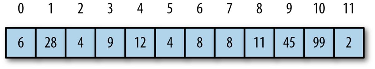
Figure 3-1. Lists as indexed slots
Many functional languages have a slightly different perspective on lists, and fortunately Groovy shares this perspective. Instead of thinking of a list as indexed slots, think of it as a combination of the first element in the list (the head) plus the remainder of the list (the tail), as shown inFigure 3-2.
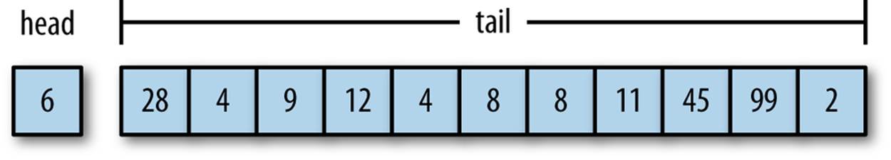
Figure 3-2. A list as its head and tail
Thinking about a list as head and tail allows me to iterate through it using recursion, as shown in Example 3-20.
Example 3-20. List traversal using recursion
def recurseList(listOfNums) {
if (listOfNums.size == 0) return;
println "${listOfNums.head()}"
recurseList(listOfNums.tail())
}
println "\nRecurse List"
recurseList(numbers)
In the recurseList() method in Example 3-20, I first check to see if the list that’s passed as the parameter has no elements in it. If that’s the case, then I’m done and can return. If not, I print out the first element in the list, available via Groovy’s head() method, and then recursively call the recurseList() method on the remainder of the list.
Recursion often has technical limits built into the platform, so this technique isn’t a panacea. But it should be safe for lists that contain a small number of items.
I’m more interested in investigating the impact on the structure of the code, in anticipation of the day when the limits ease or disappear, as they always do as languages evolve (see Chapter 5). Given the shortcomings, the benefit of the recursive version might not be immediately obvious. To make it more so, consider the problem of filtering a list. In Example 3-21, I show a filtering method that accepts a list and a predicate (a Boolean test) to determine if the item belongs in the list.
Example 3-21. Imperative filtering with Groovy
def filter(list, predicate) {
def new_list = []
list.each {
if (predicate(it)) {
new_list << it
}
}
return new_list
}
modBy2 = { n -> n % 2 == 0}
l = filter(1..20, modBy2)
println l
The code in Example 3-21 is straightforward: I create a holder variable for the elements that I want to keep, iterate over the list, check each element with the inclusion predicate, and return the list of filtered items. When I call filter(), I supply a code block specifying the filtering criteria.
Consider a recursive implementation of the filter method from Example 3-21, shown in Example 3-22.
Example 3-22. Recursive filtering with Groovy
def filterR(list, pred) {
if (list.size() == 0) return list
if (pred(list.head()))
[] + list.head() + filterR(list.tail(), pred)
else
filterR(list.tail(), pred)
}
println "Recursive Filtering"
println filterR(1..20, {it % 2 == 0})
//// [2, 4, 6, 8, 10, 12, 14, 16, 18, 20]
In the filter() method in Example 3-22, I first check the size of the passed list and return it if it has no elements. Otherwise, I check the head of the list against my filtering predicate; if it passes, I add it to the list (with an initial empty list to make sure that I always return the correct type); otherwise, I recursively filter the tail.
The difference between Examples 3-21 and 3-22 highlights an important question: Who’s minding the state? In the imperative version, I am. I must create a new variable named new_list, I must add things to it, and I must return it when I’m done. In the recursive version, the languagemanages the return value, building it up on the stack as the recursive return for each method invocation. Notice that every exit route of the filter() method in Example 3-22 is a return call, which builds up the intermediate value on the stack. You can cede responsibility for new_list; the language is managing it for you.
NOTE
Recursion allows you to cede state management to the runtime.
The same filtering technique illustrated in Example 3-22 is a natural fit for a functional language such as Scala, which combines currying and recursion, shown in Example 3-23.
Example 3-23. Recursive filtering in Scala
objectCurryTestextendsApp {
def filter(xs:List[Int], p:Int => Boolean):List[Int] =
if (xs.isEmpty) xs
elseif (p(xs.head)) xs.head :: filter(xs.tail, p)
else filter(xs.tail, p)
def dividesBy(n:Int)(x:Int) = ((x % n) == 0) // ![]()
val nums =List(1, 2, 3, 4, 5, 6, 7, 8)
println(filter(nums, dividesBy(2))) // ![]()
println(filter(nums, dividesBy(3)))
}
![]()
Function is defined to be curried.
![]()
filter expects as parameters a collection (nums) and a function that accepts a single parameter (the curried dividesBy() function).
The list-construction operators in Scala make the return conditions for both cases quite readable and easy to understand. The code in Example 3-23 is one of the examples of both recursion and currying from the Scala documentation. The filter() method recursively filters a list of integers via the parameter p, a predicate function—a common term in the functional world for a Boolean function. The filter() method checks to see if the list is empty and, if it is, simply returns; otherwise, it checks the first element in the list (xs.head) via the predicate to see if it should be included in the filtered list. If it passes the predicate condition, the return is a new list with the head at the front and the filtered tail as the remainder. If the first element fails the predicate test, the return becomes solely the filtered remainder of the list.
Although not as dramatic a life improvement as garbage collection, recursion does illustrate an important trend in programming languages: offloading moving parts by ceding it to the runtime. If I’m never allowed to touch the intermediate results of the list, I cannot introduce bugs in the way that I interact with it.
TAIL-CALL OPTIMIZATION
One of the major reasons that recursion isn’t a more commonplace operation is stack growth. Recursion is generally implemented to place intermediate results on the stack, and languages not optimized for recursion will suffer stack overflow. Languages such as Scala and Clojure have worked around this limitation in various ways. One particular way that developers can help runtimes handle this problem is tail-call optimization. When the recursive call is the last call in the function, runtimes can often replace the results on the stack rather than force it to grow.
Many functional languages (such as Erlang), implement tail recursion without stack growth. Tail recursion is used to implement long-running Erlang processes that act as microservices within the application, receiving messages from other processes and carrying out tasks on their behalf as directed by those messages. The tail-recursive loop receiving and acting on messages also allows for the maintenance of state internal to the microservice, because any effects on the current state, which is immutable, can be reflected by passing a new state variable to the next recursion. Given Erlang’s impressive fault-tolerance capabilities, there are likely tail-recursive loops in production that have run for years uninterrupted.
My guess is that you don’t use recursion at all now—it’s not even a part of your tool box. However, part of the reason lies in the fact that most imperative languages have lackluster support for it, making it more difficult to use than it should be. By adding clean syntax and support, functional languages make recursion a candidate for simple code reuse.
Streams and Work Reordering
One of the advantages of switching from an imperative to a functional style lies in the runtime’s ability to make efficiency decisions for you.
Consider the Java 8 version of the “company process” from Chapter 2, repeated in Example 3-24 with a slight difference.
Example 3-24. Java 8 version of the company process
public String cleanNames(List<String> names) {
if (names == null) return "";
return names
.stream()
.map(e -> capitalize(e))
.filter(n -> n.length() > 1)
.collect(Collectors.joining(","));
}
Astute readers will notice that I changed the order of operations in this version of cleanNames() (in contrast to Example 2-4 in Chapter 2), putting the map() operation before filter(). When thinking imperatively, the instinct is to place the filtering operation before the mapping operation, so that the map has less work to perform, filtering a smaller list. However, many functional languages (including Java 8 and even the Functional Java framework) define a Stream abstraction. A Stream acts in many ways like a collection, but it has no backing values, and instead uses a stream of values from a source to a destination. In Example 3-24, the source is the names collection and the destination (or “terminal”) is collect(). Between these operations, both map() and filter() are lazy, meaning that they defer execution as long as possible. In fact, they don’t try to produce results until a downstream terminal “asks” for them.
For the lazy operations, intelligent runtimes can reorder the result of the operation for you. In Example 3-24, the runtime can flip the order of the lazy operations to make it more efficient, performing the filtering before the mapping. As with many functional additions to Java, you must ensure that the lambda blocks you pass to functions such as filter() don’t have side effects, which will lead to unpredictable results.
Allowing the runtime to optimize when it can is another great example of ceding control: giving away mundane details and focusing on the problem domain rather than the implementation of the problem domain.
I discuss laziness in more detail in Chapter 4 and Java 8 streams in Chapter 7.