Multiplayer Game Programming: Architecting Networked Games (2016)
Chapter 2. The Internet
This chapter provides an overview of the TCP/IP suite and the associated protocols and standards involved in Internet communication, including a deep dive into those which are most relevant for multiplayer game programming.
Origins: Packet Switching
The Internet as we know it today is a far cry from the four-node network as which it started life in late 1969. Originally known as ARPANET, it was developed by the United States Advanced Research Projects Agency with the stated goal of providing geographically dispersed scientists with access to uniquely powerful computers, similarly geographically dispersed.
ARPANET was to accomplish its goal using a newly invented technology called packet switching. Before the advent of packet switching, long-distance systems transmitted information through a process known as circuit switching. Systems using circuit switching sent information via a consistent circuit, created by dedicating and assembling smaller circuits into a longer path that persisted throughout the duration of the transmission. For instance, to send a large chunk of data, like a telephone call, from New York to Los Angeles, the circuit switching system would dedicate several smaller lines between intermediary cities to this chunk of information. It would connect them into a continuous circuit, and the circuit would persist until the system was done sending the information. In this case, it might reserve a line from New York to Chicago, a line from Chicago to Denver, and a line from Denver to Los Angeles. In reality these lines themselves consisted of smaller dedicated lines between closer cities. The lines would remain dedicated to this information until the transmission was complete; that is, until the telephone call was finished. After that the system could dedicate the lines to other information transmissions. This provided a very high quality of service for information transfer. However, it limited the usability of the lines in place, as the dedicated lines could only be used for one purpose at a time, as shown in Figure 2.1.
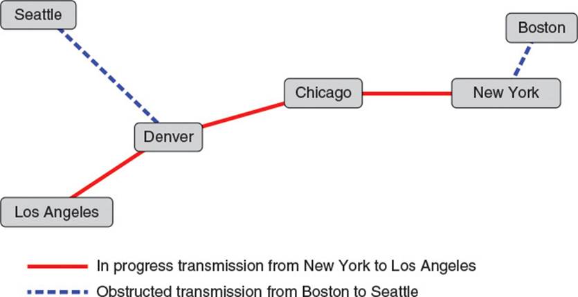
Figure 2.1 Circuit switching
Packet switching, however, provides increased usability by removing the requirement that a circuit be dedicated to a single transmission at a time. It achieves this by breaking up transmissions into small chunks called packets and sending them down shared lines using a process called store and forward. Each node of the network is connected to other nodes in the network using a line that can carry packets between the nodes. Each node can store incoming packets and then forward them to a node closer to their final destination. For instance, in the call from New York to Los Angeles, the call would be broken up into very short packets of data. They would then be sent from New York to Chicago. When the Chicago node receives a packet, it examines the packet’s destination and decides to forward the packet to Denver. The process continues until the packets arrive in Los Angeles and then the call receiver’s telephone. The important distinction from circuit switching is that other phone conversations can happen at the same time, using the same lines. Other calls from New York to Los Angeles could have their packets forwarded along the same lines at the same time, as could a call from Boston to Seattle, or anywhere in between. Lines can hold packets from many, many transmissions at once, increasing usability, as shown in Figure 2.2.
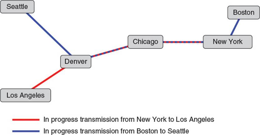
Figure 2.2 Packet switching
Packet switching itself is just a concept, though. Nodes on the network need a formal protocol collection to actually define how data should be packaged into packets and forwarded throughout the network. For the ARPANET, this protocol collection was defined in a paper known as the BBN Report 1822 and referred to as the 1822 protocol. Over many years, the ARPANET grew and grew and became part of the larger network now known as the Internet. During this time the protocols of the 1822 report evolved as well, becoming the protocols that drive the Internet of today. Together, they form a collection of protocols now known as the TCP/IP suite.
The TCP/IP Layer Cake
The TCP/IP suite is at once both a beautiful and frightening thing. It is beautiful because in theory it consists of a tower of independent and well-abstracted layers, each supported by a variety of interchangeable protocols, bravely fulfilling their duties to support dependent layers and relay their data appropriately. It is frightening because these abstractions are often flagrantly violated by protocol authors in the name of performance, expandability, or some other worthwhile yet complexity-inducing excuse.
As multiplayer game programmers, our job is to understand the beauty and horror of the TCP/IP suite so that we can make our game functional and efficient. Usually this involves touching only the highest layers of the stack, but to do that effectively, it is useful to understand the underlying layers and how they affect the layers above them.
There are multiple models which explain the interactions of the layers used for Internet communication. RFC 1122, which defined early Internet host requirements, uses four layers: the link layer, the IP layer, the transport layer, and the application layer. The alternate Open Systems Interconnection (OSI) model uses seven layers: the physical layer, the data link layer, the network layer, the transport layer, the session layer, the presentation layer, and the application layer. To focus on matters relevant to game developers, this book uses a combined, five-model layer, consisting of the physical layer, the link layer, the network layer, the transport layer, and the application layer, as shown in Figure 2.3. Each layer has a duty, supporting the needs of the layer directly above it. Typically that duty includes
![]() Accepting a block of data to transmit from a higher layer
Accepting a block of data to transmit from a higher layer
![]() Packaging the data up with a layer header and sometimes a footer
Packaging the data up with a layer header and sometimes a footer
![]() Forwarding the data to a lower layer for further transmission
Forwarding the data to a lower layer for further transmission
![]() Receiving transmitted data from a lower layer
Receiving transmitted data from a lower layer
![]() Unpackaging transmitted data by removing the header
Unpackaging transmitted data by removing the header
![]() Forwarding transmitted data to a higher layer for further processing
Forwarding transmitted data to a higher layer for further processing
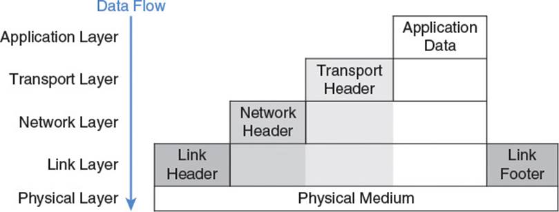
Figure 2.3 A game developer’s view of the TCP/IP layer cake
The way a layer performs its duty, however, is not built into the definition of the layer. In fact, there are various protocols each layer can use to do its jobs, with some as old as the TCP/IP suite and others currently being invented. For those familiar with object-oriented programming, it can be useful to think of each layer as an interface, and each protocol or collection of protocols as an implementation of that interface. Ideally, the details of a layer’s implementation are abstracted away from the higher layers in the suite, but as mentioned previously that is not always true. The rest of this chapter presents an overview of the layers of the suite and some of the most common protocols employed to implement them.
The Physical Layer
At the very bottom of the layer cake is the most rudimentary, supporting layer: the physical layer. The physical layer’s job is to provide a physical connection between networked computers, or hosts. A physical medium is necessary for the transmission of information. Twisted pair Cat 6 cable, phone lines, coaxial cable, and fiber optic cable are all examples of physical media that can provide the connection required by the physical layer.
Note that it is not necessary that the physical connection be tangible. As anyone with a mobile phone, tablet, or laptop can attest, radio waves also provide a perfectly good physical medium for the transmission of information. Some day soon, quantum entanglement may provide a physical medium for the transmission of information across great distances at instantaneous speeds, and when it does, the great layer cake of the Internet will be ready to accept it as a suitable implementation of its physical layer.
The Link Layer
The link layer is where the real computer science of the layer cake begins. Its job is to provide a method of communication between physically connected hosts. This means the link layer must provide a method through which a source host can package up information and transmit it through the physical layer, such that the intended destination host has a sporting chance of receiving the package and extracting the desired information.
At the link layer, a single unit of transmission is known as a frame. Using the link layer, hosts send frames to each other. Broken down more specifically, the duties of the link layer are to
![]() Define a way for a host to be identified such that a frame can be addressed to a specific destination.
Define a way for a host to be identified such that a frame can be addressed to a specific destination.
![]() Define the format of a frame that includes the destination address and the data to be sent.
Define the format of a frame that includes the destination address and the data to be sent.
![]() Define the maximum size of a frame so that higher layers know how much data can be sent in a single transmission.
Define the maximum size of a frame so that higher layers know how much data can be sent in a single transmission.
![]() Define a way to physically convert a frame into an electronic signal that can be sent over the physical layer and probably received by the intended host.
Define a way to physically convert a frame into an electronic signal that can be sent over the physical layer and probably received by the intended host.
Note that delivery of the frame to the intended host is only probable, not guaranteed. There are many factors which influence whether the electronic signal actually arrives uncorrupted at its intended destination. A disruption in the physical medium, some kind of electrical interference, or an equipment failure could cause a frame to be dropped and never delivered. The link layer does not promise any effort will be made to determine if a frame arrives or resend it if it does not. For this reason, communication at the link layer level is referred to as unreliable. Any higher-layer protocol that needs guaranteed, or reliable, delivery of data must implement that guarantee itself.
For each physical medium which can be chosen to implement the physical layer, there is a corresponding protocol or list of protocols which provide the services necessary at the link layer. For instance, hosts connected by twisted pair cable can communicate using one of the Ethernet protocols such as 1000BASET. Hosts connected by radio waves can communicate using one of the short-range Wi-Fi protocols (e.g., 802.11g, 802.11n, 802.11ac) or one of the longer-range wireless protocols such as 3G or 4G. Table 2.1 lists some popular physical medium and link layer protocol combinations.
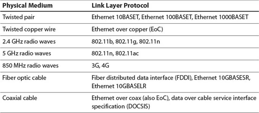
Table 2.1 Physical Medium and Link Layer Protocol Pairings
Because the link layer implementation and physical layer medium are so closely linked, some models group the two into a single layer. However, because some physical media support more than one link layer protocol, it can be useful to think of them as different layers.
It is important to note that an Internet connection between two distant hosts does not simply involve a single physical medium and a single link layer protocol. As will be explained in the following sections in the discussion of the remaining layers, several media and link layer protocols may be involved in the transmission of a single chunk of data. As such, many of the link layer protocols listed in the table may be employed while transmitting data for a networked computer game. Luckily, thanks to the abstraction of the TCP/IP suite, the details of the link layer protocols used are mostly hidden from the game. Therefore, we will not explore in detail the inner workings of each of the existing link layer protocols. However, above all the rest, there is one link layer protocol group which both clearly illustrates the function of the link layer and is almost guaranteed to impact the working life of a networked game programmer in some way, and that is Ethernet.
Ethernet/802.3
Ethernet is not just a single protocol. It is a group of protocols all based on the original Ethernet blue book standard, published in 1980 by DEC, Intel, and Xerox. Collectively, modern Ethernet protocols are now defined under IEEE 802.3. There are varieties of Ethernet which run over fiber optic cable, twisted pair cable, or straight copper cable. There are varieties that run at different speeds: As of this writing, most desktop computers support gigabit speed Ethernet but 10 GB Ethernet standards exist and are growing in popularity.
To assign an identity to each host, Ethernet introduces the idea of the media access control address or MAC address. A MAC address is a theoretically unique 48-bit number assigned to each piece of hardware that can connect to an Ethernet network. Usually this hardware is referred to as anetwork interface controller or NIC. Originally, NICs were expansion cards, but due to the prevalence of the Internet, they have been built into most motherboards for the last few decades. When a host requires more than one connection to a network, or a connection to multiple networks, it is still common to add additional NICs as expansion cards, and such a host then has multiple MAC addresses, one for each NIC.
To keep MAC addresses universally unique, the NIC manufacturer burns the MAC address into the NIC during hardware production. The first 24 bits are an organizationally unique identifier or OUI, assigned by the IEEE to uniquely identify the manufacturer. It is then the manufacturer’s responsibility to ensure the remaining 24 bits are uniquely assigned within the hardware it produces. In this way, each NIC produced should have a hardcoded, universally unique identifier by which it can be addressed.
The MAC address is such a useful concept that it is not used in just Ethernet. It is in fact used in most IEEE 802 link layer protocols, including Wi-Fi and Bluetooth.
Note
Since its introduction, the MAC address has evolved in two significant ways. First, it is no longer reliable as a truly unique hardware identifier, as many NICs now allow software to arbitrarily change their MAC address. Second, to remedy a variety of pending issues, the IEEE has introduced the concept of a 64-bit MAC style address, called the extended unique identifier or EUI64. Where necessary, a 48-bit MAC address can be converted to an EUI64 by inserting the 2 bytes FFFE right after the OUI.
With a unique MAC address assigned to each host, Figure 2.4 specifies the format for an Ethernet packet, which wraps an Ethernet link layer frame.
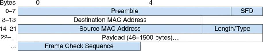
Figure 2.4 Ethernet packet structure
The Preamble and start frame delimiter (SFD) are the same for each packet and consist of the hex bytes 0×55 0×55 0×55 0×55 0×55 0×55 0×55 0×D5. This is a binary pattern that helps the underlying hardware sync up and prepare for the incoming frame. The Preamble and SFD are usually stripped from the packet by the NIC hardware, and the remaining bytes, comprising the frame, are passed to the Ethernet module for processing.
After the SFD are 6 bytes which represent the MAC address of the intended recipient of the frame. There is a special destination MAC address, FF:FF:FF:FF:FF:FF, known as the broadcast address, which indicates that the frame is intended for all hosts on the local area network.
The length/type field is overloaded and can be used to represent either length or type. When the field is used to represent length, it holds the size in bytes of the payload contained in the frame. However, when it is used to represent type, it contains an EtherType number which uniquely identifies the protocol that should be used to interpret the data inside the payload. When the Ethernet module receives this field, it must determine the correct way to interpret it. To assist with interpretation, the Ethernet standard defines the maximum length of the payload as 1500 bytes. This is known as the maximum transmission unit, or MTU, because it is the maximum amount of data that can be conveyed in a single transmission. The standard also defines the minimum EtherType value to be 0x0600, which is 1536. Thus, if the length/type field contains a number ≤1500, it represents a length, and if it contains a number ≥1536, it represents a protocol type.
Note
Although not a standard, many modern Ethernet NICs support frames with MTUs higher than 1500 bytes. These jumbo frames can often have MTUs up to 9000 bytes. To support this, they specify an EtherType in the frame header and then rely on the underlying hardware to compute the size of the frame based on incoming data.
The payload itself is the data transmitted by this frame. Typically it is a network layer packet, having been passed onto the link layer for delivery to the appropriate host.
The frame check sequence (FCS) field holds a cyclic redundancy check (CRC32) value generated from the two address fields, the length/type field, the payload, and any padding. This way, as the Ethernet hardware reads in data, it can check for any corruption that occurred in transit and discard the frame if it did. Although Ethernet does not guarantee delivery of data, it makes a good effort to prevent delivery of corrupted data.
The specifics of the manner in which Ethernet packets are transmitted along the physical layer vary between media and are not relevant to the multiplayer game programmer. It suffices to say that each host on the network receives the frame, at which point the host reads the frame and determines if it is the intended recipient. If so, it extracts the payload data and processes it accordingly based on the value of the length/type field.
Note
Initially, most small Ethernet networks used hardware known as hubs to connect multiple hosts together. Even older networks used a long coaxial cable strung between computers. In these style networks, the electronic signal for the Ethernet packet was literally sent to each host on the network, and it was up to the host to determine whether the packet was addressed to that host or not. This proved inefficient as networks grew. With the cost of hardware declining, most modern networks now use devices known as switches to connect hosts. Switches remember the MAC addresses, and sometimes the IPs, of the hosts connected to each of their ports, so most packets can be sent on the shortest path possible to their intended recipient, without having to visit every host on the network.
The Network Layer
The link layer provides a clear way to send data from an addressable host to one or more similarly addressable hosts. Therefore, it may be unclear why the TCP/IP suite requires any further layers. It turns out the link layer has several shortcomings which require a superior layer to address:
![]() Burned in MAC addresses limit hardware flexibility. Imagine you have a very popular webserver that thousands of users visit each day via Ethernet. If you were only using the link layer, queries to the server would need to be addressed via the MAC address of its Ethernet NIC. Now imagine that one day the NIC explodes in a very small ball of fire. When you install a replacement NIC, it will have a different MAC address, and thus your server will no longer receive requests from users. Clearly you need some easily configurable address system that lives on top of the MAC address.
Burned in MAC addresses limit hardware flexibility. Imagine you have a very popular webserver that thousands of users visit each day via Ethernet. If you were only using the link layer, queries to the server would need to be addressed via the MAC address of its Ethernet NIC. Now imagine that one day the NIC explodes in a very small ball of fire. When you install a replacement NIC, it will have a different MAC address, and thus your server will no longer receive requests from users. Clearly you need some easily configurable address system that lives on top of the MAC address.
![]() The link layer provides no support for segmenting the Internet into smaller, local area networks. If the entire Internet were run using just the link layer, all computers would have to be connected in a single continuous network. Remember that Ethernet delivers each frame to every host on the network and allows the host to determine if it is the intended recipient. If the Internet used only Ethernet for communication, then each frame would have to travel to every single wired host on the planet. A few too many packets could bring the entire Internet to its knees. Also, there would be no ability to sanction different areas of the network into different security domains. It can be useful to easily broadcast a message to just the hosts in a local office, or just share files with the various computers in a house. With just the link layer there would be no ability to do this.
The link layer provides no support for segmenting the Internet into smaller, local area networks. If the entire Internet were run using just the link layer, all computers would have to be connected in a single continuous network. Remember that Ethernet delivers each frame to every host on the network and allows the host to determine if it is the intended recipient. If the Internet used only Ethernet for communication, then each frame would have to travel to every single wired host on the planet. A few too many packets could bring the entire Internet to its knees. Also, there would be no ability to sanction different areas of the network into different security domains. It can be useful to easily broadcast a message to just the hosts in a local office, or just share files with the various computers in a house. With just the link layer there would be no ability to do this.
![]() The link layer provides no inherent support for communication between hosts using different link layer protocols. The fundamental idea behind allowing multiple physical and link layer protocols is that different networks can use the best implementation for their particular job. However, link layer protocols define no way of communicating from one link layer protocol to another. Again, you find yourself requiring an address system which sits on top of the hardware address system of the link layer.
The link layer provides no inherent support for communication between hosts using different link layer protocols. The fundamental idea behind allowing multiple physical and link layer protocols is that different networks can use the best implementation for their particular job. However, link layer protocols define no way of communicating from one link layer protocol to another. Again, you find yourself requiring an address system which sits on top of the hardware address system of the link layer.
The network layer’s duty is to provide a logical address infrastructure on top of the link layer, such that host hardware can easily be replaced, groups of hosts can be segregated into subnetworks, and hosts on distant subnetworks, using different link layer protocols and different physical media can send messages to each other.
IPv4
Today, the most common protocol used to implement the required features of the network layer is Internet protocol version 4 or IPv4. IPv4 fulfills its duties by defining a logical addressing system to name each host individually, a subnet system for defining logical subsections of the address space as physical subnetworks, and a routing system for forwarding data between subnets.
IP Address and Packet Structure
At the heart of IPv4 is the IP address. An IPv4 IP address is a 32-bit number, usually displayed to humans as four 8-bit numbers separated with periods. For example, the IP address of www.usc.edu is 128.125.253.146 and the IP address of www.mit.edu is 23.193.142.184. When read aloud, the periods are usually pronounced, “dot.” With a unique IP address for each host on the Internet, a source host can direct a packet to a destination host simply by specifying the destination host’s IP address in the header of the packet. There is an exception to IP address uniqueness, explained later in the section “Network Address Translation.”
With the IP address defined, IPv4 then defines the structure of an IPv4 packet. The packet consists of a header, containing data necessary for implementing network layer functionality, and a payload, containing a higher layer’s data to be transferred. Figure 2.5 gives the structure for an IPv4 packet.
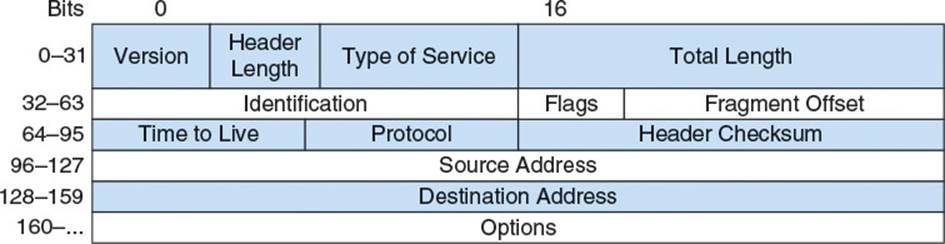
Figure 2.5 IPv4 header structure
Version (4 bits) specifies which version of the IP this packet supports. For IPv4, this is 4.
Header length (4 bits) specifies the length of the header in 32-bit words. Due to the optional fields at the end of an IP header, the header may be a variable length. The length field specifies exactly when the header ends and the encapsulated data begins. Because the length is specified in only 4 bits, it has a maximum value of 15, which means a header can be a maximum of 15 32-bit words, or 60 bytes. Because there are 20 bytes of mandatory information in the header, this field will never be less than 5.
Type of service (8 bits) is used to for a variety of purposes ranging from congestion control to differentiated services identification. For more information, see RFC 2474 and RFC 3168 in the “Additional Reading” section.
Packet length (16 bits) specifies the length in bytes of the entire packet, including header and payload. As the maximum number representable with 16 bits is 65535, the maximum packet size is clamped at 65535. As the minimum size of an IP header is 20 bytes, this means the maximum payload conveyable in an IPv4 packet is 65515 bytes.
Fragment identification (16 bits), fragment flags (3 bits), and fragment offset (13 bits), are used for reassembling fragmented packets, as explained later in the section “Fragmentation.”
Time to live or TTL (8 bits) is used to limit the number of times a packet can be forwarded, as explained later in the section “Subnets and Indirect Routing.”
Protocol (8 bits) specifies the protocol which should be used to interpret the contents of the payload. This is similar to the EtherType field in an Ethernet frame, in that it classifies a higher layer’s encapsulated data.
Header checksum (16 bits) specifies a checksum that can be used to validate the integrity of the IPv4 header. Note that this is only for the header data. It is up to a higher layer to ensure integrity of the payload if required. Often, this is unnecessary, as many link layer protocols already contain a checksum to ensure integrity of their entire frame; for example, the FCS field in the Ethernet header.
Source address (32 bits) is the IP address of the packet’s sender, and destination address (32 bits) is either the IP address of the packet’s destination host, or a special address specifying delivery to more than one host.
Note
The confusing manner of specifying header length in 32-bit words, but packet length in 8-bit words, suggests how important it is to conserve bandwidth. Because all possible headers are a multiple of 4-bytes long, their byte lengths are all evenly divisible by 4, and thus the last 2 bits of their byte lengths are always 0. Thus specifying the header length as units of 32-bit words saves 2 bits. Conserving bandwidth when possible is a golden rule of multiplayer game programming.
Direct Routing and Address Resolution Protocol
To understand how IPv4 allows packets to travel between networks with different link layer protocols, one must first understand how it delivers packets within a single network with a single link layer protocol. IPv4 allows packets to be targeted using an IP address. For the link layer to deliver a packet to the proper destination, it needs to be wrapped in a frame with an address the link layer can understand. Consider how Host A would send data to Host B in the network in Figure 2.6.
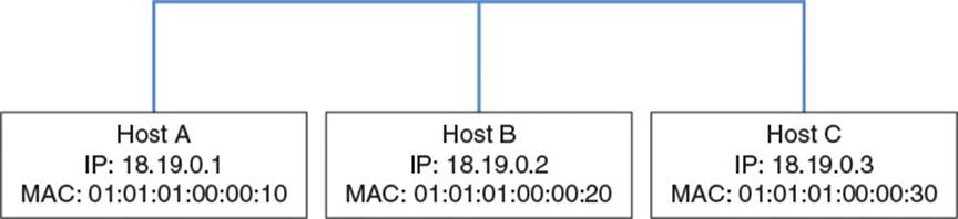
Figure 2.6 Three-host network
The sample network shown in Figure 2.6 contains three hosts, each with a single NIC, all connected by Ethernet. Host A wants to send a network layer packet to Host B at its IP address of 18.19.0.2. So, Host A prepares an IPv4 packet with a source IP address of 18.19.0.1 and a destination IP address of 18.19.0.2. In theory, the network layer should then hand off the packet to the link layer to perform the actual delivery. Unfortunately, the Ethernet module cannot deliver a packet purely by IP address, as IP is a network layer concept. The link layer needs some way to figure out the MAC address which corresponds to IP address 18.19.0.2. Luckily, there is a link layer protocol called the address resolution protocol (ARP), which provides a method for doing just that.
Note
ARP is technically a link layer protocol because it sends out packets directly using link layer style addresses and does not require the routing between networks provided by the network layer. However, because the protocol violates some network layer abstractions by including network layer IP addresses, it can be useful to think of it more as a bridge between the layers than as a solely link layer protocol.
ARP consists of two main parts: a packet structure for querying the MAC address of the NIC associated with a particular IP address, and a table for keeping track of those pairings. A sample ARP table is shown in Table 2.2.
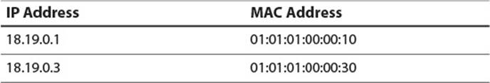
Table 2.2 An ARP Table Mapping from IP Address to MAC Address
When the IP implementation needs to send a packet to a host using the link layer, it must first query the ARP table to fetch the MAC address associated with the destination IP address. If it finds the MAC address in the table, the IP module constructs a link layer frame using that MAC address and passes the frame to the link layer implementation for delivery. However, if the MAC address is not in the table, the ARP module attempts to determine the proper MAC address by sending out an ARP packet (Figure 2.7) to all reachable hosts on the link layer network.
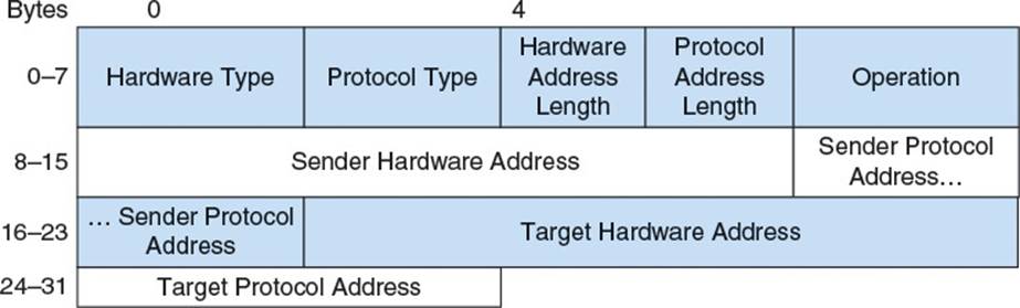
Figure 2.7 ARP packet structure
Hardware type (16 bits) defines the type of hardware on which the link layer is hosted. For Ethernet, this is 1.
Protocol type (16 bits) matches the EtherType value of the network layer protocol being used. For instance, IPv4 is 0×0800.
Hardware address length (8 bits) is the length in bytes of the link layer’s hardware address. In most cases, this would be the MAC address size of 6 bytes.
Protocol address length (8 bits) is the length in bytes of the network layer’s logical address. For IPv4, this is the IP address size of 4 bytes.
Operation (16 bits) is either 1 or 2, specifying whether this packet is a request for information (1) or a response (2).
Sender hardware address (variable length) is the hardware address of the sender of this packet and sender protocol address (variable length) is the network layer address of the sender of this packet. The lengths of these addresses match the lengths specified earlier in the packet.
Target hardware address (variable length) and target protocol address (variable length) are the corresponding addresses of the intended recipient of this packet. In the case of a request, the target hardware address is unknown and ignored by the receiver.
Continuing the previous example, if Host A doesn’t know the MAC address of Host B, it prepares an ARP request packet with 1 in the Operation field, 18.19.0.1 in the sender protocol address field, 01:01:01:00:00:10 in the sender hardware field, and 18.19.0.2 in the target protocol address field. It then wraps this ARP packet in an Ethernet frame, which it sends to the Ethernet broadcast address FF:FF:FF:FF:FF:FF. Recall that this address specifies that the Ethernet frame should be delivered to and examined by each host on the network.
When Host C receives the packet, it does not respond because its IP address does not match the target protocol address in the packet. However, when Host B receives the packet, its IP does, so it responds with its own ARP packet containing its own addresses as the source and Host A’s addresses as the target. When Host A receives the packet, it updates its ARP table with Host B’s MAC address, and then wraps the waiting IP packet in an Ethernet frame and sends it off to Host B’s MAC address.
Note
When Host A broadcasts its initial ARP request to all hosts on the network, it includes both its MAC address and IP address. This gives all the other hosts on the network an opportunity to update their ARP tables with Host A’s information even though they don’t need it yet. This comes in handy if they ever have to talk to Host A, as they won’t have to send out an ARP request packet first.
You may notice this system creates an interesting security vulnerability! A malicious host can send out ARP packets claiming to be any IP at all. Without a way to verify the authenticity of the ARP information, a switch might unintentionally route packets intended for one host to the malicious host. This not only allows sniffing packets, but could prevent intercepted packets from ever arriving at their intended host, thoroughly disrupting traffic on the network.
Subnets and Indirect Routing
Imagine two large companies, Company Alpha and Company Bravo. They each have their own large internal networks, Network Alpha and Network Bravo, respectively. Network Alpha contains 100 hosts, Host A1 to A100, and Network Bravo contains 100 hosts, Host B1 to B100. The two companies would like to connect their networks so they can send occasional messages back and forth, but simply connecting the networks with an Ethernet cable at the link layer presents a couple problems. Remember that an Ethernet packet must travel to each connected host on a network. Connecting Networks Alpha and Bravo at the link layer would cause each Ethernet packet to travel to 200 hosts instead of 100, effectively doubling the traffic on the entire network. It also presents a security risk, as it means all of Network Alpha’s packets travel to Network Bravo, not just the ones intended for Network Bravo’s hosts.
To allow Company Alpha and Company Bravo to connect their networks efficiently, the network layer introduces the ability to route packets between hosts on networks not directly connected at the link layer level. In fact, the Internet itself was originally conceived as a federation of such smaller networks throughout the country, joined by a few long-distance connections between them. The “inter” prefix on Internet, meaning, “between,” represents these connections. It is the network layer’s job to make this interaction between networks possible. Figure 2.8 illustrates a network layer connection between Networks Alpha and Bravo.
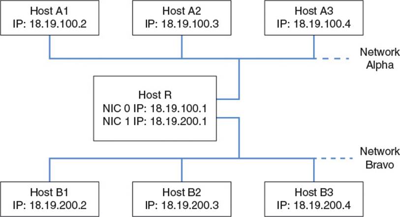
Figure 2.8 Connected networks Alpha and Bravo
Host R is a special type of host known as a router. A router has multiple NICs, each with its own IP address. In this case, one is connected to Network Alpha, and the other is connected to Network Bravo. Notice that all the IP addresses on Network Alpha share the prefix 18.19.100 and all the addresses on Network Bravo share the prefix 18.19.200. To understand why this is useful to our cause, we must now explore the subnet in more detail and define the concept of a subnet mask.
A subnet mask is a 32-bit number, usually written in the four-number, dotted notation typical of IP addresses. Hosts are said to be on the same subnet if their IP addresses, when bitwise ANDed with the subnet mask, yield the same result. For instance, if a subnet is defined as having a mask of 255.255.255.0, then 18.19.100.1 and 18.19.100.2 are both valid IP addresses on that subnet (Table 2.3). However, 18.19.200.1 is not on the subnet because it yields a different result when bitwise ANDed with the subnet mask.
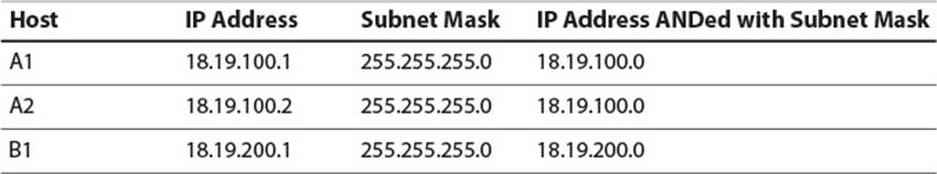
Table 2.3 IP Addresses and Subnet Masks
In binary form, subnet masks are usually a string of 1s followed by a string of 0s, as this makes them easily human readable and human bitwise ANDable. Table 2.4 lists typical subnet masks and the number of unique hosts possible on the subnet. Note that two addresses on a subnet are always reserved and not usable by hosts. One is the network address, which is formed by bitwise ANDing the subnet mask with any IP address on the subnet. The other is the broadcast address, which is formed by bitwise ORing the network address with the bitwise complement of the subnet mask. That is, every bit in the network address that does not define the subnet should be set to 1. Packets addressed to the broadcast address for a subnet should be delivered to every host on the subnet.
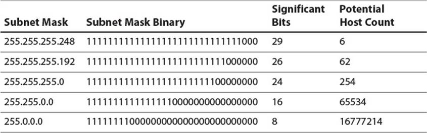
Table 2.4 Sample Subnet Masks
Because a subnet is, by definition, a group of hosts with IP addresses that yield the same result when bitwise ANDed with a subnet mask, a particular subnet can be defined simply by its subnet mask and network address. For instance, the subnet of Network Alpha is defined by network address 18.19.100.0 with subnet mask 255.255.255.0.
There is a common way to abbreviate this information, and that is known as classless inter-domain routing (CIDR) notation. A subnet mask in binary form is typically n ones followed by (32–n) zeroes. Therefore, a subnet can be notated as its network address followed by a forward slash and then the number of significant bits set in its subnet mask. For instance, the subnet of Network Alpha in Figure 2.8 is written using CIDR notation as 18.19.100.0/24.
Note
The “classless” term in CIDR comes from the fact that inter-domain routing and address block assignment used to be based on three specifically sized classes of network. Class A networks had a subnet mask of 255.0.0.0, Class B networks had a subnet mask of 255.255.0.0, and Class C networks had a subnet mask of 255.255.255.0. For more on the evolution to CIDR, see RFC 1518 mentioned in the “Additional Reading” section.
With subnets defined, the IPv4 specification provides a way to move packets between hosts on different networks. This is made possible by the routing table present in the IP module of each host. Specifically, when the IPv4 module of a host is asked to send an IP packet to a remote host, it must decide whether to use the ARP table and direct routing, or some indirect route. To aid in this process, each IPv4 module contains a routing table. For each reachable destination subnet, the routing table contains a row with information on how packets should be delivered to that subnet. For the network in Figure 2.8, potential routing tables for Hosts A1, B1, and R are given in Tables 2.5, 2.6, and 2.7.
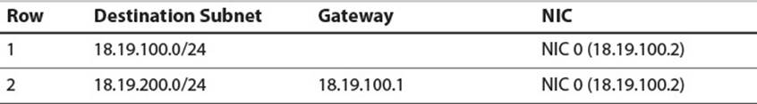
Table 2.5 Host A1 Routing Table
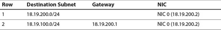
Table 2.6 Host B1 Routing Table
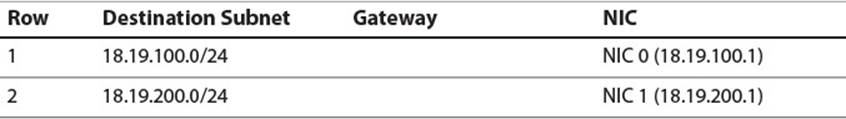
Table 2.7 Host R Routing Table
The destination subnet column refers to the subnet which contains the target IP address. The gateway column refers to the IP address of the next host, on the current subnet, which should be sent this packet via the link layer. It is required that this host be reachable through direct routing. If the gateway field is blank, it means the entire destination subnet is reachable through direct routing and the packet can be sent directly via the link layer. Finally, the NIC column identifies the NIC which should actually forward the packet. This is the mechanism by which a packet can be received from one link layer network and forwarded to another.
When Host A1 at 18.19.100.2 attempts to send a packet to Host B1 at 18.19.200.2, the following process occurs:
1. Host A1 builds an IP packet with source address 18.19.100.2 and destination address 18.19.200.2.
2. Host A1’s IP module runs through the rows of its routing table from top to bottom, until it finds the first one with a destination subnet that contains the IP address 18.19.200.2. In this case, that is row 2. Note that the order of the rows is significant, as multiple rows might match a given address.
3. The gateway listed in row 2 is 18.19.100.1, so Host A1 uses ARP and its Ethernet module to wrap the packet in an Ethernet frame and send it to the MAC address that matches IP address 18.19.100.1. This arrives at Host R.
4. Host R’s Ethernet module, running for its NIC 0 with IP address 18.19.100.1, receives the packet, detects the payload is an IP packet, and passes it up to its IP module.
5. Host R’s IP module sees the packet is addressed to 18.19.200.1, so it attempts to forward the packet to 18.19.200.1.
6. Host R’s IP module runs through its routing table until it finds a row whose destination subnet contains 18.19.200.1. In this case that is row 2.
7. Row 2 has no gateway, which means the subnet is directly routable. However, the NIC column specifies the use of the NIC 1 with IP address 18.19.200.1. This is the NIC connected to Network Bravo.
8. Host R’s IP module passes the packet to the Ethernet module running for Host R’s NIC 1. It uses ARP and the Ethernet module to wrap the packet in an Ethernet frame and send it to the MAC address that matches IP 18.19.200.1.
9. Host B1’s Ethernet module receives the packet, detects the payload is an IP packet, and passes it up to its IP module.
10. Host B1’s IP module sees that the destination IP address is its own. It sends the payload up to the next layer for more processing.
This example shows how two carefully configured networks communicate through indirect routing, but what if these networks need to send packets to the rest of the Internet? In that case, they first need a valid IP address and gateway from an Internet Service Provider (ISP). For our purposes, assume they are assigned an IP address of 18.181.0.29 and a gateway of 18.181.0.1 by the ISP. The network administrator must then install an additional NIC into Host R and configure it with the IP address assigned. Finally, she must update the routing tables on Host R and all hosts on the network. Figure 2.9 shows the new network configuration and Tables 2.8, 2.9, and 2.10 show amended routing tables.
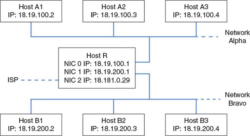
Figure 2.9 Networks Alpha and Bravo connected to the Internet
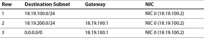
Table 2.8 Host A1 Routing Table with Internet Access
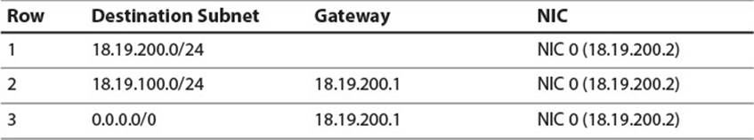
Table 2.9 Host B1 Routing Table with Internet Access
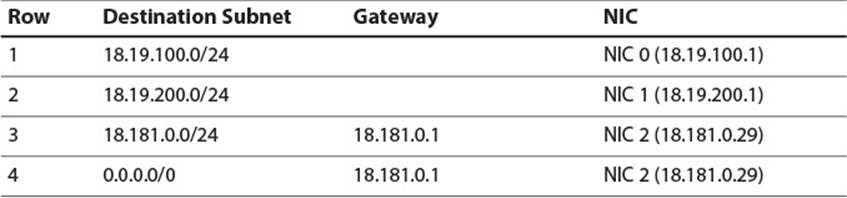
Table 2.10 Host R Routing Table with Internet Access
Note
An ISP is not a special construct as far as the Internet is concerned. It’s just a large organization, with its own very large block of IP addresses. What makes it interesting is that its main job is to take those IP addresses, break them into subnets, and then lease the subnets out to other organizations for use.
The destination 0.0.0.0/0 is known as the default address, because it defines a subnet which contains all IP addresses. If Host R receives a packet for a destination which does not match any of the first three rows, the destination will definitely match the subnet in the final row. In that case, the packet will be forwarded, via the new NIC, to the ISP’s gateway, which should be able to set the packet on a path, from gateway to gateway, which will eventually terminate at the packet’s intended destination. Similarly, Hosts A1 and B1 have new entries with the default address as their destination so that they can route Internet packets to Host R, which can then route them to the ISP.
Each time a packet is sent to a gateway and forwarded, the TTL field in the IPv4 header is decreased. When the TTL reaches 0, the packet is dropped by whichever host’s IP module did the final decrementing. This prevents packets from circling the Internet forever if there happens to be cyclical routing information on the route. Changing the TTL requires recalculating the header checksum, which contributes to the time it takes hosts to process and forward a packet.
A TTL of 0 is not the only reason a packet might be dropped. For instance, if packets arrive at a router’s NIC too rapidly for the NIC to process them, the NIC might just ignore them. Alternatively if packets arrive at a router on several NICs, but all need to be forwarded through a single NIC which isn’t fast enough to handle them, some might be dropped. These are just some of the reasons an IP packet might be dropped on its journey from source to destination. As such, all protocols in the network layer, including IPv4, are unreliable. This means there is no guarantee that IPv4 packets, once sent, will arrive at their intended destination. Even if the packets do arrive, there is no guarantee they will arrive in their intended order, or that they will only arrive once. Network congestion may cause a router to route one packet onto one path and another packet with the same destination onto another path. These paths might be different lengths and thus cause the latter packet to arrive first. Sometimes the same packet might get sent on multiple routes, causing it to arrive once and then arrive again a little later! Unreliability means no guarantee of delivery or delivery order.
Important IP Addresses
There are two special IP addresses worth mentioning. The first is the loopback or localhost address, 127.0.0.1. If an IP module is asked to send a packet to 127.0.0.1, it doesn’t send it anywhere. It instead acts as if it just received the packet, and sends it up to the next layer for processing. Technically, the entire 127.0.0.0/8 address block should loopback, but some operating systems have firewall defaults which allow only packets addressed to 127.0.0.1 to do so completely.
The next is the zero network broadcast address, 255.255.255.255. This indicates the packet should be broadcast to all hosts on the current local link layer network but should not be passed through any routers. This is usually implemented by wrapping the packet in a link layer frame and sending it to the broadcast MAC address FF:FF:FF:FF:FF:FF.
Fragmentation
As mentioned earlier, the MTU, or maximum payload size, of an Ethernet frame is 1500 bytes. However, as noted previously, the maximum size of an IPv4 packet is 65535 bytes. This raises a question: If an IP packet must be transmitted by wrapping it in a link layer frame, how can it ever be larger than the link layer’s MTU? The answer is fragmentation. If an IP module is asked to transmit a packet larger than the MTU of the target link layer, it can break the packet up into as many MTU-sized fragments as necessary.
IP packet fragments are just like regular IP packets, but with some specific values set in their headers. They make use of the fragment identification, fragment flags, and fragment offset fields of the header. When an IP module breaks an IP packet into a group of fragments, it creates a new IP packet for each fragment and sets the fields accordingly.
The fragment identification field (16 bits) holds a number which identifies the originally fragmented packet. Each fragment in a group has the same number in this field.
The fragment offset field (13 bits) specifies the offset, in 8-byte blocks, from the start of the original packet to the location in which this fragment’s data belongs. This is necessarily a different number for each fragment within the group. The crazy numbering scheme is chosen so that any possible offset within a 65535-byte packet can be specified with only 13 bits. This requires that all offsets be even multiples of 8 bytes, because there is no ability to specify an offset with greater precision than that.
The fragment flags field (3 bits) is set to 0x4 for every fragment but the final fragment. This number is called the more fragments flag, representing that there are more fragments in the fragment group. If a host receives a packet with this flag set, it must wait until all fragments in the group are received before passing the reassembled packet up to a higher layer. This flag is not necessary on the final fragment, because it has a nonzero fragment offset field, similarly indicating that it is a member of a fragment group. In fact, the flag must be left off the final fragment to indicate that there are no further fragments in the original packet.
Note
The fragment flags field has one other purpose. The original sender of an IP packet can set this to 0x2, a number known as the do not fragment flag. This specifies that the packet should not be fragmented under any circumstances. Instead, if an IP module must forward the packet on a link with an MTU smaller than the packet size, the packet should be dropped instead of fragmented.
Table 2.11 shows the relevant header fields for a large IP packet and the three packets into which it must be fragmented in order to forward it over an Ethernet link.
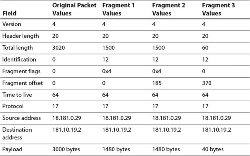
Table 2.11 IPv4 Packet Which Must Be Fragmented
The fragment identification fields are all 12, indicating that the three fragments are all from the same packet. The number 12 is arbitrary, but it’s likely this is the 12th fragmented packet this host has sent. The first fragment has the more fragments flag set and a packet offset of 0, indicating that it contains the initial data from the unfragmented packet. Note that the packet length field indicates a total length of 1500. The IP module usually chooses to create fragments as large as possible to limit the number of fragments. Because the IP header is 20 bytes, this leaves 1480 for the fragment data. That suggests the second fragment’s data should start at an offset of 1480. However, because the fragment offset field is represented in 8-byte blocks, and 1480/8 is 185, the actual number contained there is 185. The more fragments flag is also set on the second fragment. Finally, the third fragment has a data offset of 370 and does not have the more fragments flag set, indicating it is the final fragment. The total length of the third fragment is only 60, as the original packet had 3000 bytes of data inside its total length of 3020. Out of this 1480 bytes are in the first fragment, 1480 are in the second, and 40 are in the third.
After these fragment packets are sent out, it is conceivable that any or all of them could be further fragmented. This would happen if the route to the destination host involves traveling along a link layer with an even smaller MTU.
For the packet to be properly processed by the intended recipient, each of the packet fragments has to arrive at that final host and be reconstructed into the original, unfragmented packet. Because of network congestion, dynamically changing routing tables, or other reasons, it is possible that the packets arrive out of order, potentially interleaved with other packets from the same or other hosts. Whenever the first fragment arrives, the recipient’s IP module has enough information to establish that the fragment is indeed a fragment and not a complete packet: This is evident from either the more fragments flag being set or the nonzero packet offset field. At this point, the recipient’s IP module creates a 64-kB buffer (maximum packet size) and copies data from the fragment into the buffer at the appropriate offset. It tags the buffer with the sender’s IP address and the fragment identification number, so that when future fragments come in with a matching sender and fragment identification, the IP module can fetch the appropriate buffer and copy in the new data. When a fragment arrives without the more fragments flag set, the recipient calculates the total length of the original packet by adding that fragment’s data length to its packet offset. When all data for a packet has arrived, the IP module passes the fully reconstructed packet up to the next layer for further processing.
Tip
Although IP packet fragmentation makes it possible to send giant packets, it introduces two large inefficiencies. First, it actually increases the amount of data which must be sent over the network. Table 2.11 illustrates that a 3020-byte packet gets fragmented into two 1500-bytes packets and a 60-byte packet, for a total of 3060 bytes. This isn’t a terrible amount, but it can add up. Second, if a single fragment is lost in transit, the receiving host must drop the entire packet. This makes it more likely that larger packets with many fragments get dropped. For this reason, it is generally advisable to avoid fragmentation entirely by making sure all IP packets are smaller than the link layer MTU. This is not necessarily easy, because there can be several different link layer protocols in between two hosts: Imagine a packet traveling from New York to Japan. It is very likely that at least one of the link layers between the two hosts will use Ethernet, so game developers make the approximation that the minimum MTU of the entire packet route will be 1500 bytes. This 1500 bytes must encapsulate the 20-byte IP header, the IP payload, and any additional data required by wrapper protocols like VPN or IPSec that may be in use. For this reason, it is wise to limit IP payloads to around 1300 bytes.
At first thought, it may seem better to limit packet size to something even smaller, like 100 bytes. After all, if a 1500-byte packet is unlikely to require fragmentation, a 100-byte packet is even less likely to require it, right? This may be true, but remember that each packet requires a header of 20 bytes. A game sending out packets that are only 100 bytes in length is spending 20% of its bandwidth on just IP headers, which is very inefficient. For this reason, once you’ve decided that there is a very good chance the minimum MTU is 1500, you want to send out packets that are as close to 1500 in size as possible. This would mean that only 1.3% of your bandwidth is wasted on IP headers, which is much better than 20%!
IPv6
IPv4, with its 32-bit addresses, allows for 4 billion unique IP addresses. Thanks to private networks and network address translation (discussed later in this chapter) it is possible for quite a few more hosts than that to actively communicate on the Internet. Nevertheless, due to the way IP addresses are allotted, and the proliferation of PCs, mobile devices, and the Internet of Things, the world is running out of 32-bit IP addresses. IPv6 was created to address both this problem, and some inefficiencies that have become evident throughout the long life of IPv4.
For the next few years, IPv6 will probably remain of low importance to game developers. As of July 2014, Google reports that roughly 4% of its users access its site through IPv6, which is probably a good indication of how many end users in general are using devices connecting to the Internet through IPv6. As such, games still have to handle all the idiosyncrasies and oddities of IPv4 that IPv6 was designed to fix. Nevertheless, as next gen platforms like the Xbox One gain in popularity, IPv6 will eventually replace IPv4, and it is worth briefly exploring what IPv6 is all about.
The most noticeable new feature of IPv6 is its new IP address length of 128 bits. IPv6 addresses are written as eight groups of 4-digit hex numbers, separated by colons. Table 2.12 shows a typical IPv6 address in three accepted forms.
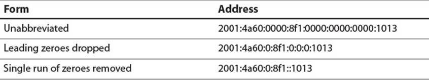
Table 2.12 Typical IPv6 Address Forms
When written, leading zeroes in each hextet may be dropped. Additionally, a single run of zeroes may be abbreviated with a double colon. Because the address is always 16 bytes, it is simple to reconstruct the original form by replacing all missing digits with zeroes.
The first 64 bits of an IPv6 address typically represent the network and are called the network prefix, whereas the final 64 bits represent the individual host and are called the interface identifier. When it is important for a host to have a consistent IP address, such as when acting as a server, a network administrator may manually assign the interface identifier, similar to how IP addresses are manually assigned for IPv4. A host that does not need to be easy to find by remote clients can also chose its interface identifier at random and announce it to the network, as chances of a collision in the 64-bit space are low. Most often, the interface identifier is automatically set to the NIC’s EUI-64, as this is already guaranteed to be unique.
Neighbor discovery protocol (NDP) replaces ARP as well as some of the features of DHCP, as described later in this chapter. Using NDP, routers advertise their network prefixes and routing table information, and hosts query and announce their IP addresses and link layer addresses. More information on NDP can be found in RFC 4861, referenced in the “Additional Reading” section.
Another nice change from IPv4 is that IPv6 no longer supports packet fragmentation at the router level. This enables the removal of all the fragmentation-related fields from the IP header and saves some bandwidth on each packet. If an IPv6 packet reaches a router and is too big for the outgoing link layer, the router simply drops the packet and responds to the sender that the packet was too big. It is up to the sender to try again with a smaller packet.
More information on IPv6 can be found in RFC 2460, referenced in the “Additional Reading” section.
The Transport Layer
While the network layer’s job is to facilitate communication between distant hosts on remote networks, the transport layer’s job is to enable communication between individual processes on those hosts. Because multiple processes can be running on a single host, it is not always enough to know that Host A sent an IP packet to Host B: When Host B receives the IP packet, it needs to know which process should be passed the contents for further processing. To solve this, the transport layer introduces the concept of ports. A port is a 16-bit, unsigned number representing a communication endpoint at a particular host. If the IP address is like a physical street address of a building, a port is a bit like a suite number inside that building. An individual process can then be thought of as a tenant who can fetch the mail from one or more suites inside that building. Using a transport layer module, a process can bind to a specific port, telling the transport layer module that it would like to be passed any communication addressed to that port.
As mentioned, all ports are 16-bit numbers. In theory, a process can bind to any port and use it for any communicative purpose it wants. However, problems arise if two processes on the same host attempt to bind to the same port. Imagine that both a webserver program and an email program bind to port 20. If the transport layer module receives data for port 20, should it deliver that data to both processes? If so, the webserver might interpret incoming email data as a web request, or the email program might interpret an incoming web request as email. This will end up making either a web surfer, or an emailer very confused. For this reason, most implementations require special flags for multiple processes to bind the same port.
To help avoid processes squabbling over ports, a department of the Internet Corporation for Assigned Names and Numbers (ICANN) known as the Internet Assigned Numbers Authority (IANA) maintains a port number registry with which various protocol and application developers can register the ports their applications use. There is only a single registrant per port number per transport layer protocol. Port numbers 1024-49151 are known as the user ports or registered ports. Any protocol and application developer can formally request a port number from this range from IANA, and after a review process, the port registration may be granted. If a user port number is registered with the IANA for a certain application or protocol, then it is considered bad form for any other application or protocol implementation to bind to that port, although most transport layer implementations do not prevent it.
Ports 0 to 1023 are known as the system ports or reserved ports. These ports are similar to the user ports, but their registration with IANA is more restricted and subject to more thorough review. These ports are special because most operating systems allow only root level processes to bind system ports, allowing them to be used for purposes requiring elevated levels of security.
Finally, ports 49152 to 65535 are known as dynamic ports. These are never assigned by IANA and are fair game for any process to use. If a process attempts to bind to a dynamic port and finds that it is in use, it should handle that gracefully by attempting to bind to other dynamic ports until an available one is found. As a good Internet citizen, you should use only dynamic ports while building your multiplayer games, and then register with IANA for a user port assignment if necessary.
Once an application has identified a port to use, it must employ a transport layer protocol to actually send data. Sample transport layer protocols, as well as their IP protocol number, are listed in Table 2.13. As game developers we deal primarily with UDP and TCP.
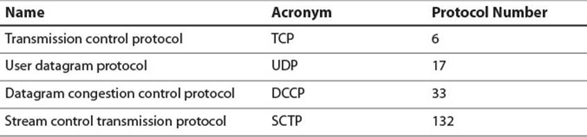
Table 2.13 Examples of Transport Layer Protocols
Tip
IP addresses and ports are often combined with a colon to indicate a complete source or destination address. So, a packet heading to IP 18.19.20.21 and port 80 would have its destination written as 18.19.20.21:80.
UDP
User datagram protocol (UDP) is a lightweight protocol for wrapping data and sending it from a port on one host to a port on another host. A UDP datagram consists of an 8-byte header followed by the payload data. Figure 2.10 shows the format of a UDP header.

Figure 2.10 UDP header
Source port (16 bits) identifies the port from which the datagram originated. This is useful if the recipient of the datagram wishes to respond.
Destination port (16 bits) is the target port of the datagram. The UDP module delivers the datagram to whichever process has bound this port.
Length (16 bits) is the length of the UDP header and payload.
Checksum (16 bits) is an optional checksum calculated based on the UDP header, payload, and certain fields of the IP header. If not calculated, this field is all zeroes. Often this field is ignored because lower layers validate the data.
UDP is very much a no-frills protocol. Each datagram is a self-contained entity, relying on no shared state between the two hosts. It can be thought of as a postcard, dropped in the mail, and then forgotten. UDP provides no effort to limit traffic on a clogged network, deliver data in order, or guarantee that data is delivered at all. This is all very much in contrast to the next transport layer we will explore, TCP.
TCP
Whereas UDP allows the transfer of discreet datagrams between hosts, transmission control protocol (TCP) enables the creation of a persistent connection between two hosts followed by the reliable transfer of a stream of data. The key word here is reliable. Unlike every protocol discussed so far, TCP does its best to ensure all data sent is received, in its intended order, at its intended recipient. To effect this, it requires a larger header than UDP, and nontrivial connection state tracking at each host participating in the connection. This enables recipients to acknowledge received data, and senders to resend any transmissions that are unacknowledged.
A TCP unit of data transmission is called a TCP segment. This refers to the fact that TCP is built for transmitting a large stream of data and each lower layer packet wraps a single segment of that stream. A segment consists of a TCP header followed by the data for that segment. Figure 2.11shows its structure.
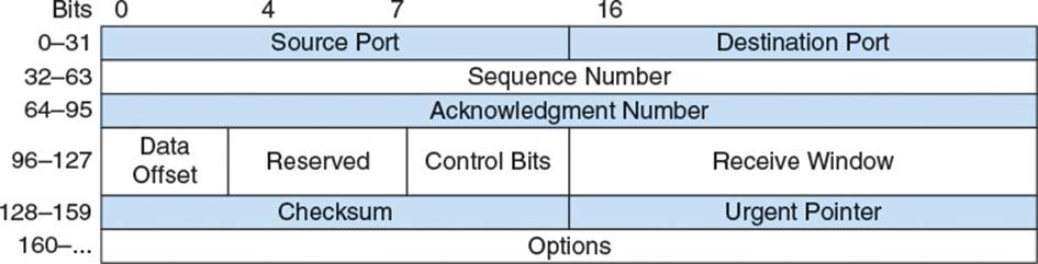
Figure 2.11 TCP header
Source port (16 bits) and destination port (16 bits) are transport layer port numbers.
Sequence number (32-bits) is a monotonically increasing identifier. Each byte transferred via TCP has a consecutive sequence number which serves as a unique identifier of that byte. This way, the sender can label data being sent and the recipient can acknowledge it. The sequence number of a segment is typically the sequence number of the first byte of data in that segment. There is an exception when establishing the initial connection, as explained in the “Three-Way Handshake” section.
Acknowledgment number (32-bits) contains the sequence number of the next byte of data that the sender is expecting to receive. This acts as a de facto acknowledgment for all data with sequence numbers lower than this number: Because TCP guarantees all data is delivered in order, the sequence number of the next byte that a host expects to receive is always one more than the sequence number of the previous byte that it has received. Be careful to remember that the sender of this number is not actually acknowledging receipt of the sequence number with this value, but actually of all sequence numbers lower than this value.
Data offset (4 bits) specifies the length of the header in 32-bit words. TCP allows for some optional header elements at the end of its header, so there can be from 20 to 64 bytes between the start of the header and the data of the segment.
Control bits (9 bits) hold metadata about the header. They are discussed later where relevant.
Receive window (16 bits) conveys the maximum amount of remaining buffer space the sender has for incoming data. This is useful for maintaining flow control, as discussed later.
Urgent pointer (16 bits) holds the delta between the first byte of data in this segment and the first byte of urgent data. This is only relevant if the URG flag is set in the control bits.
Note
Instead of using the loosely defined “byte” to refer to 8 bits, many RFCs, including those that define the major transport layer protocols, unambiguously refer to 8-bit sized chunks of data as octets. Some legacy platforms used bytes that contained more or fewer than 8 bits, and the standardization around an octet of bits helped ensure compatibility between platforms. This is less of an issue these days, as all platforms relevant to game developers treat a byte as 8 bits.
Reliability
Figure 2.12 illustrates the general manner in which TCP brings about reliable data transfer between two hosts. In short, the source host sends a uniquely identified packet to the destination host. It then waits for a response packet from the destination host, acknowledging receipt of the packet. If it does not receive the expected acknowledgment within a certain amount of time, it resends the original packet. This continues until all data has been sent and acknowledged.
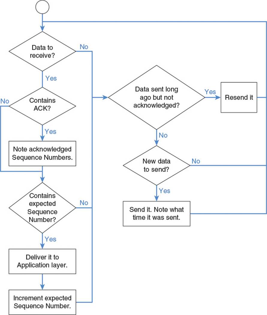
Figure 2.12 TCP reliable data transfer flow chart
The exact details of this process are slightly more complicated, but worth understanding in depth, as they provide an excellent case study of a reliable data transfer system. Because the TCP strategy involves resending data and tracking expected sequence numbers, each host must maintain state for all active TCP connections. Table 2.14 lists some of the state variables they must maintain and their standard abbreviations as defined by RFC 793. The process of initializing that state begins with a three-way handshake between the two hosts.
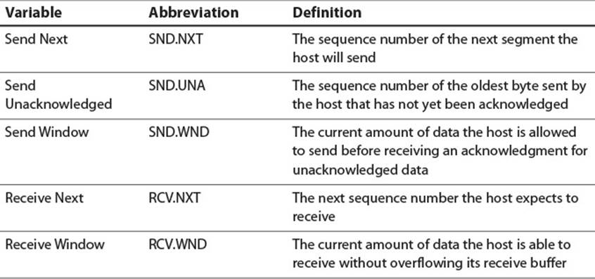
Table 2.14 TCP State Variables
Three-Way Handshake
Figure 2.13 illustrates a three-way handshake between Hosts A and B. In the figure, Host A initiates the connection by sending the first segment. This segment has the SYN flag set and a randomly chosen initial sequence number of 1000. This indicates to Host B that Host A would like to initiate a TCP connection starting at sequence number 1000, and that Host B should initialize resources necessary to maintain the connection state.
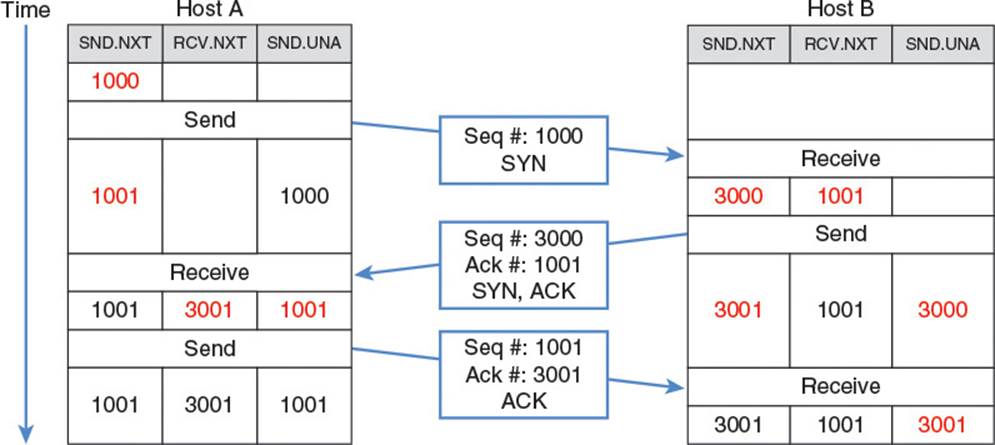
Figure 2.13 TCP three-way handshake
Host B, if it is willing and able to open the connection, then responds with a packet with both the SYN flag, and the ACK flag set. It acknowledges Host A’s sequence number by setting the acknowledgment number on the segment to Host A’s initial sequence number plus 1. This means the next segment Host B is expecting from Host A should have a sequence number one higher than the previous segment. In addition, Host B picks its own random sequence number, 3000, to start its stream of data to Host A. It is important to note that Hosts A and B each picked their own random starting sequence numbers. There are two separate streams of data involved in the connection: One from Host A to Host B, which uses Host A’s numbering, and one from Host B to Host A which uses Host B’s numbering. The presence of the SYN flag in a segment means “Hey you! I’m going to start sending you a stream of data starting with a byte labeled one plus the sequence number mentioned in this segment.” The presence of the ACK flag and the acknowledgment number in the second segment means “Oh by the way, I received all data you sent up until this sequence number, so this sequence number is what I’m expecting in the next segment you send me.” When Host A receives this segment, all that’s left is for it to ACK Host B’s initial sequence number, so it sends out a segment with the ACK flag set and Host B’s sequence number plus 1, 3001, in the acknowledgment field.
Note
When a TCP segment contains a SYN or FIN flag, the sequence number is incremented by an extra byte to represent the presence of the flag. This is sometimes known as the TCP phantom byte.
Reliability is established through the careful sending and acknowledgment of data. If a timeout expires and Host A never receives the SYN-ACK segment, it knows that Host B either never received the SYN segment, or Host B’s response was lost. Either way, Host A can resend the initial segment. If Host B did indeed receive the SYN segment and therefore receives it for a second time, Host B knows it is because Host A did not receive its SYN-ACK response, so it can resend the SYN-ACK segment.
Data Transmission
To transmit data, hosts can include a payload in each outgoing segment. Each segment is tagged with the sequence number of the first byte of data in the sequence. Remember that each byte has a consecutive sequence number, so this effectively means that the sequence number of a segment should be the sequence number of the previous segment plus the amount of data in the previous segment. Meanwhile, each time an incoming data segment arrives at its destination, the receiver sends out an acknowledgment packet with the acknowledgment field set to the next sequence number it expects to receive. This would typically be the sequence number of the most recently received segment plus the amount of data in that segment. Figure 2.14 shows a simple transmission with no dropped segments. Host A sends 100 bytes in its first segment, Host B acknowledges and sends 50 bytes of its own, Host A sends 200 bytes more, and then Host B acknowledges those 200 bytes without sending any additional data.
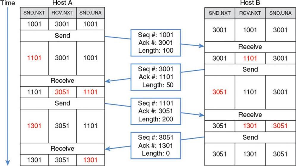
Figure 2.14 TCP transmission with no packet loss
Things get slightly more complicated when a segment gets dropped or delivered out of order. In Figure 2.15, segment 1301 traveling from Host A to Host B is lost. Host A expects to receive an ACK packet with 1301 in the acknowledgment field. When a certain time limit expires and Host A has not received the ACK, it knows something is wrong. Either segment 1301, or the ACK from Host B has been dropped. Either way, it knows it needs to redeliver segment 1301 until it receives an acknowledgment from Host B. To redeliver the segment, Host A needs to have a copy of that segment’s data on hand, and this is a key component of TCP’s operation: The TCP module must store every byte it sends out until that byte is acknowledged by the recipient. Only once an acknowledgment for a segment is received can the TCP module purge that segment’s data from its memory.
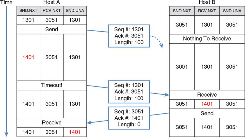
Figure 2.15 TCP packet lost and retransmitted
TCP guarantees that data is delivered in order, so if a host receives a packet with a sequence number it is not yet expecting, it has two options. The simple option is to just drop the packet and wait for it to be resent in order. An alternative option is to buffer it while neither ACKing it nor delivering it to the application layer for processing. Instead, the host copies it into its local stream buffer at the appropriate position based on the sequence number. Then, when all preceding sequence numbers have been delivered, the host can ACK the out of order packet and send it to the application layer for processing without requiring the sender to resend it.
In the preceding examples, Host A always waits for an acknowledgment before sending additional data. This is unusual and contrived just for the purpose of simplifying the examples. There is no requirement that Host A must stall its transmission, waiting for an acknowledgment after each segment it sends. In fact, if there were such a requirement, TCP would be a fairly unusable protocol over long distances.
Recall that the MTU for Ethernet is 1500 bytes. The IPv4 header takes up at least 20 of those bytes and the TCP header takes up at least another 20 bytes, which means the most data that can be sent in an unfragmented TCP segment that travels over Ethernet is 1460 bytes. This is known as the maximum segment size (MSS). If a TCP connection could only have one unacknowledged segment in flight at a time, then its bandwidth would be severely limited. In fact, it would be the MSS divided by the amount of time it takes for the segment to go from sender to receiver plus the time for the acknowledgment to return from receiver to sender (round trip time or RTT). Round trip times across the country can be on the order of 30 ms. This means the maximum cross-country bandwidth achievable with TCP, regardless of intervening link layer speed, would be 1500 bytes/0.03 seconds, or 50 kbps. That might be a decent speed for 1993, but not for today!
To avoid this problem, a TCP connection is allowed to have multiple unacknowledged segments in flight at once. However, it cannot have an unlimited number of segments in flight, as this would present another problem. When transport layer data arrives at a host, it is held in a buffer until the process which has bound the corresponding port consumes it. At that point, it is removed from the buffer. No matter how much memory is available on the host, the buffer itself is of some fixed size. It is conceivable that a complex process on a slow CPU may not consume incoming data as fast as it arrives. Thus, the buffer will fill up and incoming data will be dropped. In the case of TCP, this means the data will not be acknowledged, and the rapidly transmitting sender will then begin rapidly resending the data. In all likelihood, most of this resent data will be dropped as well, because the receiving host still has the same slow CPU and is still running the same complex process. This causes a big traffic jam and is a colossal waste of Internet resources.
To prevent this calamity, TCP implements a process known as flow control. Flow control prevents a rapidly transmitting host from overwhelming a slowly consuming one. Each TCP header contains a receive window field which specifies how much receive buffer space the sender of the packet has available. This equates to telling the other host the maximum amount of data it should send before stopping to wait for an acknowledgment. Figure 2.16 illustrates an exchange of packets between a rapidly transmitting Host A and a slowly consuming Host B.
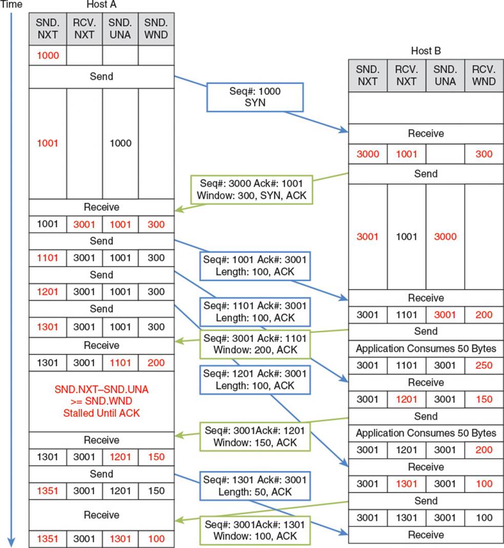
Figure 2.16 TCP flow control
For demonstration purposes, an MSS of 100 bytes is used. Host B’s initial SYN-ACK flag specifies a receive window of 300 bytes, so Host A only sends out three 100-byte segments before pausing to wait for an ACK from Host B. When Host B finally sends an ACK, it knows it now has 100 bytes in its buffer which might not be consumed quickly, so it tells Host A to limit its receive window to 200 bytes. Host A knows 200 more bytes are already on their way to B, so it doesn’t send any more data in response. It must stall until it receives an ACK from Host B. By the time Host B ACKs the second packet, 50 bytes of data from its buffer have been consumed, so it has a total of 150 bytes remaining in its buffer and 150 bytes free. When it sends an ACK to Host A, it tells Host A to limit the receive window to only 150 bytes. Host A knows at this point there are still 100 unacknowledged bytes in flight, but the receive window is 150 bytes, so it sends an additional 50-byte segment off to Host B.
Flow control continues in this way, with Host B always alerting Host A to how much data it can hold so that Host A never sends out more data than Host B can buffer. With that in mind, the theoretical bandwidth limit for a TCP stream of data is given by this equation:
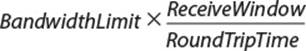
Having too small a receive window can create a bottleneck for TCP transmission. To avoid this, a large enough receive window should be chosen such that the theoretical bandwidth maximum is always greater than the maximum transmission rate of the link layer in between the hosts.
Notice that in Figure 2.16, Host B ends up sending two ACK packets in a row to Host A. This is not a very efficient use of bandwidth, as the acknowledgment number in the second ACK packet sufficiently acknowledges all the bytes that the first ACK packet acknowledges. Due to the IP and TCP headers alone, this wastes 40 bytes of bandwidth from Host B to Host A. When link layer frames are factored in, this wastes even more. To prevent this inefficiency, TCP rules allow for something called a delayed acknowledgment. According to the specification, a host receiving a TCP segment does not have to immediately respond with an acknowledgment. Instead, it can wait up to 500 ms, or until the next segment is received, whichever occurs first. In the previous example, if Host B receives the segment with sequence number 1101 within 500 ms of the segment with sequence number 1001, Host B only has to send an acknowledgment for segment 1101. For heavy data streams, this effectively cuts in half the number of required ACKs, and always gives a receiving host time to consume some data from its buffer and therefore include a larger receive window in its acknowledgments.
Flow control helps TCP protect slow endpoint consumers from being overwhelmed with data, but it does nothing to prevent slow networks and routers from being overwhelmed. Traffic builds up on networks just like it does on highways, with jams getting especially bad at popular routers, much like at popular entrances, exits, and interchanges. To avoid cluttering up networks unnecessarily, TCP implements congestion control, which is very similar to the stop light meters found at many highway entrances. To reduce congestion, the TCP module voluntarily limits the amount of unacknowledged data it will allow in flight. This is similar to what it does for flow control, but instead of setting the limit to a window size dictated by the destination, it calculates the limit itself based on the number of packets that have been acknowledged or dropped. The exact algorithm is implementation dependent, but typically is some sort of additive increase, multiplicative decrease system. That is, when a connection is established, the TCP module sets the congestion avoidance limit to a low multiple of the MSS. Choosing two times the MSS is typical. Then, for every segment acknowledged, it increases the limit by an additional MSS. For an ideal connection, this means that a limit’s worth of packets are acknowledged every RTT period, which causes the limit to double in size. However, if a packet is ever dropped, the TCP module quickly cuts the limit in half, suspecting that the drop was due to network congestion. In this way, an equilibrium is eventually reached such that a sender is transmitting as fast as it can without causing so much traffic that packets begin to drop.
TCP can also reduce network congestion by sending out packets as close in size to the MSS as necessary. Because each packet requires a 40-byte header, sending several small segments is much less efficient than coalescing the segments into a larger chunk and sending it when ready. This means the TCP module needs to keep an outgoing buffer to accumulate data that higher layers attempt to send. Nagle’s algorithm is a set of rules that many TCP implementations use to decide when to accumulate data and when to finally send a segment. Traditionally, if there is already unacknowledged data in flight, it accumulates data until the amount is greater than the MSS or congestion control window, whichever is smaller. At that point it sends the largest segment allowed by those two limits.
Tip
Nagle’s algorithm is the bane of players whose games use TCP as a transport layer protocol. Although it decreases bandwidth used, it can significantly increase the delay before data is sent. If a real-time game needs to send small updates to a server, it might be many frames of gameplay before enough updates accumulate to fill an MSS. This can leave players feeling the game is laggy even though it’s just Nagle’s algorithm at work. For this reason, most TCP implementations provide an option to disable this congestion control feature.
Disconnecting
Shutting down a TCP connection requires a termination request and acknowledgment from each end. When one host has no more data to send, it sends a FIN packet, indicating that it is ready to cease sending data. All data pending in the outdoing buffer, including the FIN packet, will be transmitted and retransmitted until acknowledged. However, the TCP module will accept no new outgoing data from a higher layer. Data can still be received from the other host, though, and all incoming data will be ACK’d. When the other side has no more data to send, it too can send a FIN packet. When a closing host has received a FIN packet from the other host and an ACK packet in response to its own FIN packet, or a timeout for the ACK has been exceeded, then the TCP module fully shuts down and deletes its connection state.
The Application Layer
At the very top of the TCP/IP layer cake is the application layer, and this is where our multiplayer game code lives. The application layer is also home to many fundamental protocols of the Internet that rely on the transport layer for end-to-end communication, and we will explore some here.
DHCP
Assigning unique IPv4 addresses to each host on a private subnet can be an administrative challenge, especially when laptops and smart phones are introduced into the mix. Dynamic host configuration protocol (DHCP) solves this problem by allowing a host to request configuration information automatically when it attaches to the network.
Upon connecting to the network, the host creates a DHCPDISCOVER message containing its own MAC address and broadcasts it using UDP to 255.255.255.255:67. Because this goes to every host on the subnet, any DHCP server present will receive the message. The DHCP server, if it has an IP address to offer the client, prepares a DHCPOFFER packet. This packet contains both the offered IP address and the MAC address of the client to be sent the offer. At this point, the client has no IP address assigned, so the server can’t directly address a packet to it. Instead, the server broadcasts the packet to the entire subnet on UDP port 68. All DHCP clients receive the packet, and each checks the MAC address in the message to determine if it is the intended recipient. When the correct client receives the message, it reads the offered IP address and decides if it would like to accept the offer. If so, it responds, via broadcast, with a DHCPREQUEST message requesting the offered address. If the offer is still available, the server responds, again via broadcast, with a DHCPACK message. This message both confirms to the client that the IP address is assigned, and conveys any additional network information necessary, such as the subnet mask, router address, and any recommended DNS name servers to use.
The exact format of DHCP packets and extended information on DHCP can be found in RFC 2131, referenced in the “Additional Reading” section.
DNS
Domain name system (DNS) protocol enables the translation of domain and subdomain names into IP addresses. When an end user wants to perform a google search, she doesn’t need to type 74.125.224.112 into her web browser, but can instead just type www.google.com. To translate the domain name into an IP address, her web browser sends a DNS query to the IP address of the name server which her computer has been configured to use.
A name server stores mappings from domain names to IP addresses. For instance, one might store that www.google.com should resolve to the IP address 74.125.224.112. There are many thousands of name servers in use on the Internet, and most are only authoritative for a small subset of the Internet’s domains and subdomains. If a name server is queried about a domain for which it is not an authority, it usually has a pointer to a more authoritative name server which it queries in turn. The results of the second query are usually cached so that the next time the name server must answer a query for that domain, it has the answer on hand.
DNS queries and responses are usually sent via UDP on port 53. The format is defined in RFC 1035, referenced in the “Additional Reading” section.
NAT
Until now, every IP address discussed has been publically routable. An IP address qualifies as publically routable if any properly configured router on the Internet can set a packet on a route such that the packet eventually arrives at the host with that IP address. This necessitates that any publically routable address be uniquely assigned to a single host. If two or more hosts shared the same IP address, then a packet addressed to one might end up at another. If one of the hosts made a request to a webserver, the response could end up at the alternate host, thoroughly confusing it.
To keep publically routable addresses unique, ICANN and its subsidiaries allocate distinct blocks of IPs to large institutions like megacorporations, universities, and Internet service providers, who can then hand out those addresses to members and customers, ensuring that each address is assigned uniquely.
Because IPv4 supports only a 32-bit address space, there are a mere 4,294,967,296 potential public IP addresses available. Due to the incredible number of networked devices in use today, and the way IP addresses are distributed by ICANN, they have grown scarce. Oftentimes, a network administrator or user may find herself allocated fewer public IP addresses than she has hosts. For instance, as video game developers, we probably each have at least a smartphone, laptop, and gaming console, yet only pay for a single public IP address from our ISP. How annoying would it be if each device required its own dedicated public IP address? Each time we connected a new gadget to the Internet, we would end up having to fight with other users for a new IP address from our ISP, and then probably pay more for it as well.
Luckily, it is possible to connect an entire subnet of hosts to the Internet through a single shared public IP address. This is made possible by network address translation or NAT. To configure a network for NAT, each host on the network must be assigned a privately routable IP address.Table 2.15 lists some IP address blocks which IANA has reserved for private use, guaranteeing that no address from those blocks will ever be assigned as a public IP address. Thus, any user may set up their own private network using privately routable IP addresses, without checking for uniqueness. Uniqueness between networks is not required because the addresses are not publically routable. That is, no public router on the Internet should have routing information regarding how to reach a private IP address, so it doesn’t matter if multiple private networks employ the same private IP addresses internally.
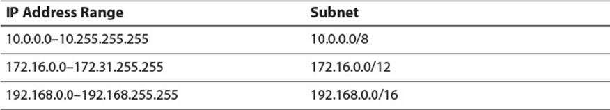
Table 2.15 Private IP Address Blocks
To understand how NAT works, consider the video gamer’s home network in Figure 2.17. The game console, smart phone, and laptop all have internally unique private IP addresses, assigned by the owner of the network, without the need to consult any outside service provider. The router also has a private IP address on its internal facing NIC, and it has a publically routable, ISP-assigned IP address on its outward facing NIC. Because the privately addressed NIC is connected to the local network, it is called a local area network (LAN) port, and because the publically addressable NIC is connected worldwide, it is called the wide area network (WAN) port.
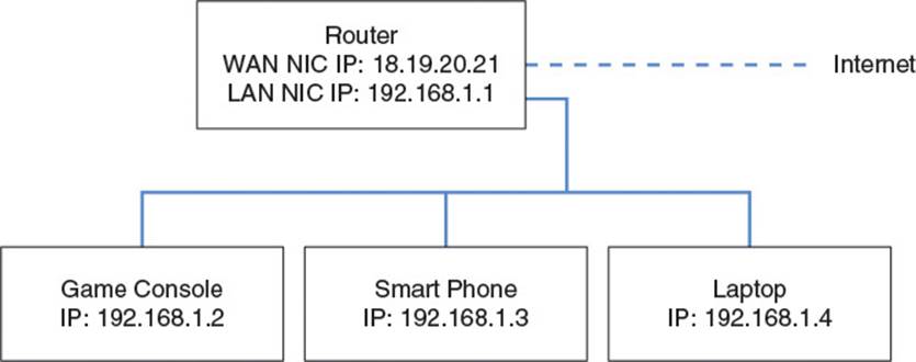
Figure 2.17 Private network behind a NAT
For this example, assume a host at the publically routable IP 12.5.3.2 is running a game server bound to port 200. The game console with private IP 192.168.1.2 is running a game bound to port 100. The game console needs to send a message to the server via UDP, so it builds a datagram as shown in Figure 2.18, with 192.168.1.2:100 as the source, and 12.5.3.2:200 as the destination. Without NAT enabled on the router, the console sends the datagram to the LAN port of the router, which then forwards it from the WAN port to the Internet. The packet eventually arrives at the server. At this point, though, there is a problem. Because the source address on the IP packet is 192.168.1.2, the server is unable to send a packet back in response. Remember that 192.168.1.2 is a private IP address, and thus no public router on the Internet can route to that address. Even if some router did nonsensically have routing information for that IP address, it is unlikely the packet would end up at our game console, as there are many thousands of hosts on the Internet with the private IP address 192.168.1.2.
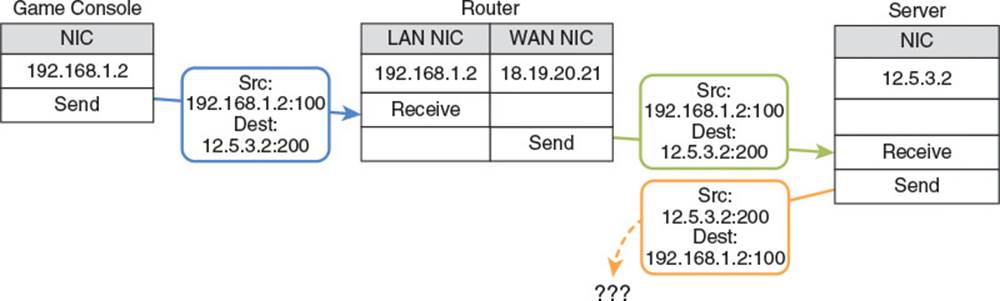
Figure 2.18 Router without NAT
To prevent this issue, the NAT module of the router can actually rewrite the IP packet as it routes it, replacing the private IP address, 192.168.1.2 with the router’s own public IP address, 18.19.20.21. That solves part of the problem but not all of it: Rewriting only the IP address creates the situation depicted in Figure 2.19. The server sees the datagram as coming directly from the router’s public IP address, so it can send a datagram back to the router successfully. However, the router has no record of who sent the original datagram, so it doesn’t know where to direct the response.
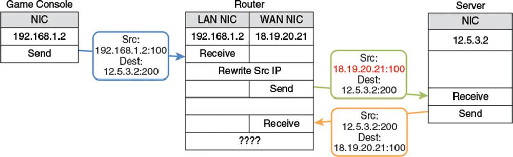
Figure 2.19 NAT router with address rewriting
To be able to return a reply to the proper internal host, the router needs some kind of mechanism to identify the intended internal recipient of an incoming packet. One naïve way is to build a table that records the source IP address of each outgoing packet. Then, when a response is received from an external IP address, the router could look up which internal host sent a packet to that address and then rewrite the packet to use that internal host’s IP address. This would break down, though, if multiple internal hosts sent traffic to the same external host. The router would not be able to identify which incoming traffic is for which internal host.
The solution employed by all modern NAT routers is to violently break the abstraction barrier between the network layer and the transport layer. By rewriting not only the IP addresses in the IP header, but also the port numbers in the transport layer header, the router can create a much more precise mapping and tagging system. It keeps track of these mapping in a NAT table. Consider Figure 2.20, which shows the traffic as a packet travels from the game console to the server and a reply returns successfully to the game console.
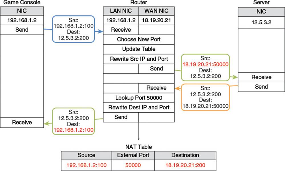
Figure 2.20 NAT router with address and port rewriting
When the game console’s outgoing packet reaches the router, the NAT module records both the source IP address and the source port number into a new row in the NAT table. It then picks a random, previously unused port number that is used to identify that source address and source port combination, and writes that number into the same row. It rewrites the packet to use the router’s own public IP address and the newly chosen port number. The rewritten packet travels to the server, at which point the server sends a response back, addressed to the router’s public IP address and newly chosen port. The NAT module then uses that port number to look up the original source IP address and port. It rewrites the response packet and forwards it to the correct host.
Note
For extra security, many routers add the original destination IP address and port to the NAT table entry. This way, when a response packet comes into the router, the NAT module can first look up the table entry using the source port of the packet and it can then make sure the source IP address and port of the response match the destination IP address and port of the original outgoing packet. If they do not match, something fishy is going on, and the packet is dropped instead of forwarded.
NAT Traversal
NAT is a fantastic boon for Internet users, but it can be a terrible headache for multiplayer game developers. Considering how many users have their own private networks at home and use NAT to connect their computers and game consoles to the Internet, it is not uncommon that the situation in Figure 2.21 arises. Player A owns Host A, behind NAT A. She wants to host a multiplayer game server on Host A. She wants her friend, Player B, to connect to her server. Player B uses Host B, behind NAT B. Because of the NAT, Player B has no way to initiate a connection with Host A. If Host B sends a packet to Host A’s router in an attempt to connect, there will be no entry in Host A’s NAT table, so the packet will simply be dropped.
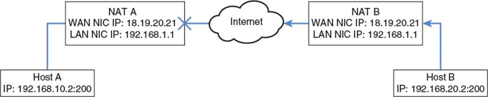
Figure 2.21 Typical user gaming setup
There are a few ways around this problem. One is to require Player A to manually configure port forwarding on her router. This is something that requires a small amount of technical skill and confidence and is not something nice to force players to do. The second way around the problem is much more elegant and much more sneaky. It is known as simple traversal of UDP through NAT or STUN.
When using STUN, hosts communicate with a third-party host, such as an Xbox Live or PlayStation Network server. That third party tells the hosts how to initiate connections with each other such that the required entries are made in their routers’ NAT tables, and they can proceed to communicate directly. Figure 2.22 shows the flow of communication, Figure 2.23 details the packets exchanged, and the NAT tables generated. Let us assume our game runs on UDP port 200 so all communication to and from non-router hosts will be on port 200.
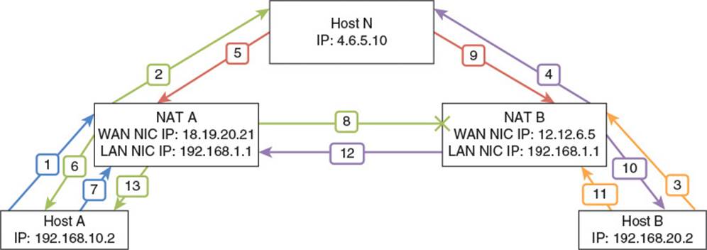
Figure 2.22 STUN data flow
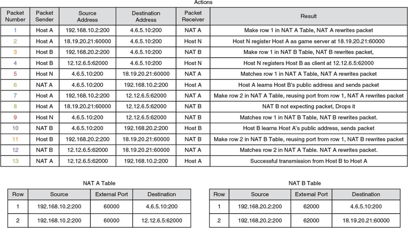
Figure 2.23 STUN packet detail and NAT tables
First, Host A sends a packet from port 200 to the negotiator service at IP 4.6.5.10 (Host N) announcing it would like to be a server. When the packet passes through Router A, Router A makes an entry in its NAT table and rewrites the packet to use its own public IP address as the source and the random number 60000 as a source port. Router A then forwards the packet to Host N. Host N receives the packet and makes note of the fact that Player A, playing on Host A, at address 18.19.20.21:60000 wants to register as a server of a multiplayer game.
Host B then sends a packet to Host N, announcing that Player B would like to connect to Player A’s game. When the packet passes through Router B, the NAT table at Router B is updated and the packet is rewritten, similar to how NAT occurred at Router A. The rewritten packet is then forwarded to Host N, who learns from the packet that Host B at 12.12.6.5:62000 would like to connect to Host A.
At this point, Host N knows Router A’s public IP address, as well as the destination port which will result in Router A forwarding a packet to Host A. It could send this information to Host B in a reply packet, and request that Host B attempt to connect directly using it. However, recall that some routers check the origin of incoming packets to make sure they are expecting packets from that location. Router A is only expecting a packet from Host N. If Host B tries to connect to Host A at this point, Router A will block the packet because Router A is not expecting any response from Host B.
Luckily, Host N also knows Router B’s public IP address and the port number which will cause a packet to be forwarded to Host B. So, it sends this information to Host A. Router A lets this information pass, because its NAT table indicates that Host A is expecting a response from Host N. Host A then sends an outgoing packet to Host B using the connection info received from Host N. This may seem crazy, as it is the server attempting to contact the client, whereas we would expect the reverse. It may seem even crazier, because we know that Router B is not expecting any incoming packets from Host A and will thus not allow the packet through anyway. Why would we waste a packet like that? We do it just to force an entry into Router A’s NAT table!
As the packet travels from Host A to Host B, it passes through Router A. Router A sees in the NAT table that Host A’s address, 192.168.1.2:200, already maps to external port 60000, so it chooses this port for the outgoing packet. It then makes an additional entry stating that 192.168.1.2:200 has sent traffic to 128.127.126.125:62000. This additional entry is the key. The packet will probably never arrive at Host B, but after this has happened, Host N can reply to Host B, telling it to connect directly to Host A at 18.19.20.21:51243. Host B does so, and when the packet arrives at Router A, Router A sees that it is indeed expecting an incoming packet from 128.127.126.125:62000. It rewrites the packet to be targeting 192.168.1.2:200 and sends it to Host A. From that point on, Hosts A and B can communicate directly by using the public IP address and port number they have exchanged.
Note
There are a few more facts about NATs worth mentioning. First, the NAT traversal technique described earlier will not work for all NATs. There are some NATs which do not assign a consistent external port number to an internal host. These are known as symmetric NATs. In a symmetric NAT, each outgoing request receives a unique external port, even if originating from a source IP address and port already in the NAT table. This breaks STUN because Router A will pick a new external port to use when Host A sends its first packet to Host B. When Host B contacts Router A on the original external port that Host A used to reach Host N, it will not match in the NAT table and the packet will be dropped.
Sometimes, less secure symmetric NATs assign external ports in a deterministic order, so clever programs can use port assignment prediction to make STUN-like techniques work on symmetric NATs. More secure symmetric NATs use randomized port assignments that cannot easily be predicted.
The STUN method works only for UDP. As described in Chapter 3, “The Berkeley Sockets,” TCP uses a different system of port assignment and necessarily transmits data on a port different from the one on which it listens for incoming connections. When TCP is in use, there is a technique called TCP hole punching which may work if the NAT router acts in a way which supports it. RFC 5128, referenced in “Additional Reading” gives a good survey of NAT traversal techniques, including TCP hole punching.
Finally, there is yet another popular way to enable traversal of a NAT router. It is called Internet gateway device protocol (IGDP). This is a protocol that some Universal Plug and Play (UPnP) routers employ to allow LAN hosts to manually set up mappings between external and internal ports. It is not always supported and less academically interesting so it is not explained here. Its specification is also referenced in the “Additional Reading” section.
Summary
This chapter provided an overview of the inner workings of the Internet. Packet switching allows multiple transmissions to be sent simultaneously over the same line, giving rise to ARPANET and eventually the Internet. The TCP/IP suite, the layer cake that powers the Internet, consists of five layers, each of which provides a data channel for the layer above it.
The physical layer provides the medium along which the signal travels, and is sometimes considered part of the link layer above it. The link layer provides a method of communication between connected hosts. It requires a hardware addressing system so that each host can be uniquely addressed, and determines the MTU, the maximum amount of data which can be transmitted in a single chunk. There are many protocols which can provide the primary link layer services, but this chapter explored Ethernet in great depth, as it is the one most important to game developers.
The network layer, which provides a logical addressing system on top of the link layer’s hardware addresses, allows hosts on different link layer networks to communicate. IPv4, the primary network layer protocol of the day, provides direct and indirect routing systems, and fragments packets too large for the link layer. IPv6, rising in prominence, solves the problem of a limited address space and optimizes several of the biggest bottlenecks in IPv4 data transmission.
The transport layer and its ports provide end-to-end communication between processes on remote hosts. TCP and UDP are the primary protocols in the transport layer, and fundamentally different: UDP is lightweight, connectionless, and unreliable, whereas TCP has a heavier footprint, requires stateful connections, and guarantees reliable, in-order delivery of all data. TCP implements flow control and congestion control mechanisms to decrease packet loss.
At the top of the cake is the application layer, containing DHCP, DNS, and your game code.
To facilitate the creation of private networks with minimal oversight, NAT allows a single public IP address to be shared by an entire network. A drawback of NAT is that it blocks unsolicited incoming connections that a server might desire, but there are techniques such as STUN and TCP hole punching which provide workarounds for this.
This chapter has provided a theoretical basis for the workings of the Internet. This will prove useful in Chapter 3, which covers the functions and data structures used to write code that actually communicates between hosts.
Review Questions
1. List the five layers of the TCP/IP stack and briefly describe each. Which layer is not considered a separate layer in some models?
2. For what is ARP used? How does it work?
3. Explain how a host with multiple NICs (i.e., a router) routes packets between different subnets. Explain how a routing table works.
4. What does MTU stand for? What does it mean? What is the MTU of Ethernet?
5. Explain how packet fragmentation works. Assuming a link layer with an MTU of 400, give the header of a packet which would be fragmented into two fragments, and then give the headers of those fragments.
6. Why is it good to avoid IP fragmentation?
7. Why is it good to send packets that are as large as possible without fragmenting?
8. What is the difference between unreliable and reliable data transfer?
9. Describe the TCP handshake process to establish a connection. What important pieces of data are exchanged?
10. Describe how TCP effects reliable data transfer.
11. What is the difference between a publically routable IP address and a privately routable one?
12. What is NAT? What are some benefits of using a NAT? What are some costs?
13. Explain how a client behind a NAT can send a packet to a publically routable server and receive a response.
14. What is STUN? Why would you need it? How does it work?
Additional Readings
Bell, Gordon. (1980, September). The Ethernet—A Local Area Network. Retrieved from http://research.microsoft.com/en-us/um/people/gbell/ethernet_blue_book_1980.pdf. Accessed September 12, 2015.
Braden, R. (Ed). (1989, October). Requirements for Internet Hosts—Application and Support. Retrieved from http://tools.ietf.org/html/rfc1123. Accessed September 12, 2015.
Braden, R. (Ed). (1989, October). Requirements for Internet Hosts—Communication Layers. Retrieved from http://tools.ietf.org/html/rfc1122. Accessed September 12, 2015.
Cotton, M., L. Eggert, J. Touch, M. Westerlund, and S. Cheshire. (2011, August). Internet Assigned Numbers Authority (IANA) Procedures for the Management of the Service Name and Transport Protocol Port Number Registry. Retrieved from http://tools.ietf.org/html/rfc6335. Accessed September 12, 2015.
Deering, S., and R. Hinden. (1998, December). Internet Protocol, Version 6 (IPv6) Specification. Retrieved from https://www.ietf.org/rfc/rfc2460.txt. Accessed September 12, 2015.
Drom, R. (1997, March). Dynamic Host Configuration Protocol. Retrieved from http://tools.ietf.org/html/rfc2131. Accessed September 12, 2015.
Google IPv6 Statistics. (2014, August 9). Retrieved from https://www.google.com/intl/en/ipv6/statistics.html. Accessed September 12, 2015.
Information Sciences Institute. (1981, September). Transmission Control Protocol. Retrieved from http://www.ietf.org/rfc/rfc793.txt. Accessed September 12, 2015.
Internet Gateway Device Protocol. (2010, December). Retrieved from http://upnp.org/specs/gw/igd2/. Accessed September 12, 2015.
Mockapetris, P. (1987, November). Domain Names—Concepts and Facilities. Retrieved from http://tools.ietf.org/html/rfc1034. Accessed September 12, 2015.
Mockapetris, P. (1987, November). Domain Names—Implementation and Specification. Retrieved from http://tools.ietf.org/html/rfc1035. Accessed September 12, 2015.
Nagle, John. (1984, January 6). Congestion Control in IP/TCP Internetworks. Retrieved from http://tools.ietf.org/html/rfc896. Accessed September 12, 2015.
Narten, T., E. Nordmark, W. Simpson, and H. Soliman. (2007, September). Neighbor Discovery for IP version 6 (IPv6). Retrieved from http://tools.ietf.org/html/rfc4861. Accessed September 12, 2015.
Nichols, K., S. Blake, F. Baker, and D. Black. (1998, December). Definition of the Differentiated Services Field (DS Field) in the IPv4 and IPv6 Headers. Retrieved from http://tools.ietf.org/html/rfc2474. Accessed September 12, 2015.
Port Number Registry. (2014, September 3). Retrieved from http://www.iana.org/assignments/service-names-port-numbers/service-names-port-numbers.xhtml. Accessed September 12, 2015.
Postel, J., and R. Reynolds. (1988, February). A Standard for the Transmission of IP Datagrams over IEEE 802 Networks. Retrieved from http://tools.ietf.org/html/rfc1042. Accessed September 12, 2015.
Ramakrishnan, K., S. Floyd, and D. Black. (September 2001). The Addition of Explicit Congestion Notification (ECN) to IP. Retrieved from http://tools.ietf.org/html/rfc3168. Accessed September 12, 2015.
Rekhter, Y., and T. Li. (1993, September ). An Architecture for IP Address Allocation with CIDR. Retrieved from http://tools.ietf.org/html/rfc1518. Accessed September 12, 2015.
Rosenberg, J., J. Weinberger, C. Huitema, and R. Mahy. (2003, March). STUN—Simple Traversal of User Datagram Protocol (UDP). Retrieved from http://tools.ietf.org/html/rfc3489. Accessed September 12, 2015.
Socolofsky, T., and C. Kale. (1991, January). A TCP/IP Tutorial. Retrieved from http://tools.ietf.org/html/rfc1180. Accessed September 12, 2015.
All materials on the site are licensed Creative Commons Attribution-Sharealike 3.0 Unported CC BY-SA 3.0 & GNU Free Documentation License (GFDL)
If you are the copyright holder of any material contained on our site and intend to remove it, please contact our site administrator for approval.
© 2016-2026 All site design rights belong to S.Y.A.