From Mathematics to Generic Programming (2015)
4. Euclid's Algorithm
The whole structure of number theory rests on a single foundation,
namely the algorithm for finding the greatest common divisor.
Dirichlet, Lectures on Number Theory
In the previous chapter, we met Pythagoras and the secretive order he founded to study astronomy, geometry, number theory, and music. While the Pythagoreans’ failure to find a common measure of the side and the diagonal of a square ended the dream of reducing the world to numbers, the idea of a greatest common measure (GCM) turned out to be an important one for mathematics—and eventually for programming. In this chapter, we’ll introduce an ancient algorithm for GCM that we’ll be exploring throughout the rest of the book.
4.1 Athens and Alexandria
To set the stage for the discovery of this algorithm, we now turn to one of the most amazing times and places in history: Athens in the 5th century BC. For 150 years following the miraculous defeat of the invading Persians in the battles of Marathon, Salamis, and Platea, Athens became the center of culture, learning, and science, laying the foundations for much of Western civilization.
It was in the middle of this period of Athenian cultural dominance that Plato founded his famous Academy. Although we think of Plato today as a philosopher, the center of the Academy’s program was the study of mathematics. Among Plato’s discoveries were what we now call the fivePlatonic solids—the only three-dimensional shapes in which every face is an identical regular polygon.
Plato (429 BC–347 BC)
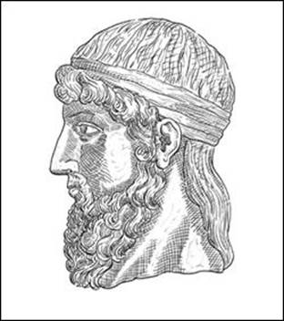
Plato was born into one of the ancient noble families of Athens. As a young man, he became a follower of Socrates, one of the founders of philosophy, who taught and learned by questioning, especially examining one’s own life and assumptions.
Socrates was ugly, bug-eyed, shabbily dressed, old, and only a lowly stonemason by trade, but his ideas were revolutionary. At the time, self-proclaimed wise men (“Sophists”) promised to teach their students to take any side of an argument and manipulate the voters. Socrates challenged the Sophists, questioning their supposed wisdom and making them look foolish. While the Sophists charged substantial fees to share their knowledge, Socrates’ followers received his training for free. To this day, the technique Socrates introduced of asking questions to get at the truth is known as the Socratic method. Although Socrates was admired by some, and some of his followers went on to be prominent leaders, he was generally considered to be a notorious troublemaker, and was publicly ridiculed in Aristophanes’ famous play Clouds. Eventually, in 399 BC, Socrates was put on trial for corrupting the city’s youth, and was condemned to death by poisoning.
Plato was profoundly influenced by Socrates, and most of his own writings take the form of dialogues between Socrates and various opponents. Plato was devastated by Socrates’ execution, and by the fact that a society would destroy its wisest and most just member. He left Athens in despair, studying for a while with the priests in Egypt, and later learning mathematics from the Pythagoreans in southern Italy. A decade or so later, he returned to Athens and founded what is essentially the world’s first university at a place called the Academy, named after an ancient hero Academus. Unlike the secret teachings of the Pythagoreans, the Academy’s program of study was public and available to everyone: men and women, Greeks and barbarians, free and slave.
Many of Plato’s dialogues, such as Apology, Phaedo, and Symposium, are as beautifully written as any poetry. Although Plato’s best-known works today are concerned with a variety of ethical and metaphysical issues, mathematics played a central role in the curriculum of the Academy. In fact, Plato had the inscription “Let no one ignorant of geometry enter” written over the entrance. He gathered many top mathematicians of the time to teach at the Academy and develop a uniform course of study. While Plato did not leave us any mathematical works, many mathematical ideas are spread throughout his dialogues, and one of them, Meno, is designed to demonstrate that mathematical reasoning is innate.
On several occasions, Plato traveled to Syracuse to influence the local ruler to introduce a just society. He was unsuccessful; in fact, one of the trips annoyed the ruler so much that he arranged for Plato to be sold into slavery. Fortunately, the philosopher was quickly ransomed by an admirer.
It is hard to exaggerate the influence of Plato on European thought. As the prominent British philosopher Whitehead said, “The safest general characterization of the European philosophical tradition is that it consists of a series of footnotes to Plato.”
Athenian culture spread throughout the Mediterranean, especially during the reign of Alexander the Great. Among his achievements, Alexander founded the Egyptian city of Alexandria (named for himself), which became the new center of research and learning. More than a thousand scholars worked in what we would now think of as a research institute, the Mouseion—the “Institution of the Muses”—from which we get our word “museum.” The scholars’ patrons were the Greek kings of Egypt, the Ptolemys, who paid their salaries and provided free room and board. Part of the Mouseion was the Library of Alexandria, which was given the task of collecting all the world’s knowledge. Supposedly containing 500,000 scrolls, the library kept a large staff of scribes busy copying, translating, and editing scrolls.
* * *
It was during this period that Euclid, one of the scholars at the Mouseion, wrote his Elements, one of the most important books in the history of mathematics. Elements includes derivations of fundamental results in geometry and number theory, as well as the ruler-and-compass constructions that students still learn today.
Euclid (flourished ca. 300 BC)
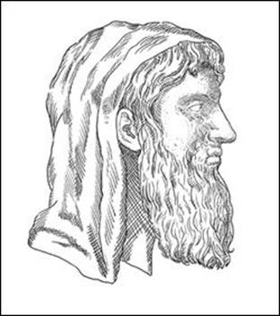
We know very little about Euclid—not even exactly when he lived. What we do know is that he took geometry very seriously. According to a story told by the philosopher Proclus Diadochus, one of Plato’s later successors as head of the Academy: “Ptolemy [the king of Egypt] once asked Euclid whether there was any shorter way to a knowledge of geometry than by study of the Elements, whereupon Euclid answered that there was no royal road to geometry.” It is probable that Euclid studied at the Academy some time after Plato’s death and brought the mathematics he learned to Alexandria.
Although we know almost nothing else about Euclid’s life, we do know about his work. His Elements incorporated mathematical results and proofs from several existing texts. A careful reading reveals some of these layers; for example, since ancient times the work on the theory of proportions in Book V has generally been believed to be based on the work of Plato’s student, Eudoxus. But it was Euclid who wove these ideas together to form a carefully crafted coherent story. In Book I, he starts with the fundamental tools for geometric construction with ruler and compass and ends with what we now call the Pythagorean Theorem (Proposition I, 47). In the 13th and final book, he shows how to construct the five Platonic solids, and proves that they are the only regular polyhedra (bodies whose faces are congruent, regular polygons) that exist.
Euclid’s Elements shows a sense of purpose unique in the history of mathematics. Each proposition and proof is there for a reason; no unnecessary results are presented. However beautiful, no theorem is presented unless it is needed for the larger story. Euclid also prefers proofs that construct as many useful results as possible with the fewest ruler-and-compass operations. His approach is reminiscent of a modern programmer striving for minimal elegant algorithms.
From its publication around 300 BC until the beginning of the 20th century, Euclid’s Elements was used as the basis of mathematical education. It was not only scientists and mathematicians who studied Euclid; great political leaders such as Thomas Jefferson and Abraham Lincoln also admired and studied Elements throughout their lives. Even now, many people believe that students would still benefit from this approach.
4.2 Euclid’s Greatest Common Measure Algorithm
Book X of Euclid’s Elements contained a concise treatment of incommensurable quantities:
Proposition 2. If, when the less of two unequal magnitudes is continually subtracted in turn from the greater, that which is left never measures the one before it, then the two magnitudes are incommensurable.
Essentially, Euclid is saying what we observed earlier in the chapter: if our procedure for computing greatest common measure never terminates, then there is no common measure.
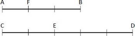
Euclid then goes on to explicitly describe the algorithm and prove that it computes the GCM. This diagram may be useful in following the proof:
Since this is the first algorithm termination proof in history, we’re including the entire text, using Sir Thomas Heath’s translation:
Proposition 3. Given two commensurable magnitudes, to find their greatest common measure.
Proof.
Let the two given commensurable magnitudes be AB, CD of which AB is the less; thus it is required to find the greatest common measure of AB, CD.
Now the magnitude AB either measures CD or it does not.
If then it measures it—and it measures itself also—AB is a common measure of AB, CD.
And it is manifest that it is also the greatest; for a greater magnitude than the magnitude AB will not measure AB.
Next, let AB not measure CD.
Then, if the less be continually subtracted in turn from the greater, that which is left over will sometime measure the one before it, because AB, CD are not incommensurable; [cf. X. 2] let AB, measuring ED, leave EC less than itself, let EC, measuring FB, leave AF less than itself, and let AF measure CE.
Since, then, AF measures CE, while CE measures FB, therefore AF will also measure FB.
But it measures itself also; therefore AF will also measure the whole AB.
But AB measures DE; therefore AF will also measure ED.
But it measures CE also; therefore it also measures the whole CD.
Therefore AF is a common measure of AB, CD.
I say next that it is also the greatest.
For, if not, there will be some magnitude greater than AF which will measure AB, CD.
Let it be G.
Since then G measures AB, while AB measures ED, therefore G will also measure ED.
But it measures the whole CD also; therefore G will also measure the remainder CE.
But CE measures FB; therefore G will also measure FB.
But it measures the whole AB also, and it will therefore measure the remainder AF, the greater [measuring] the less: which is impossible.
Therefore no magnitude greater than AF will measure AB, CD; therefore AF is the greatest common measure of AB, CD.
Therefore the greatest common measure of the two given commensurable magnitudes AB, CD has been found.
![]()
This “continual subtraction” approach to GCM is known as Euclid’s algorithm (or sometimes the Euclidean algorithm). It’s an iterative version of the gcm function we saw in Chapter 3. As we did before, we will use C++-like notation to show its implementation:
line_segment gcm0(line_segment a, line_segment b) {
while (a != b) {
if (b < a) a = a - b;
else b = b - a;
}
return a;
}
In Euclid’s world, segments cannot be zero, so we do not need this as a precondition.
Exercise 4.1. gcm0 is inefficient when one segment is much longer than the other. Come up with a more efficient implementation. Remember you can’t introduce operations that couldn’t be done by ruler-and-compass construction.
Exercise 4.2. Prove that if a segment measures two other segments, then it measures their greatest common measure.
To work toward a more efficient version of line_segment_gcm, we’ll start by rearranging, checking for b < a as long as we can:
line_segment gcm1(line_segment a, line_segment b) {
while (a != b) {
while (b < a) a = a - b;
std::swap(a, b);
}
return a;
}
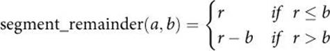
We could avoid a swap in the case where a = b, but that would require an extra test, and we’re not quite ready to optimize the code anyway. Instead, we observe that the inner while loop is computing the remainder of a and b. Let’s factor out that piece of functionality:
line_segment segment_remainder(line_segment a, line_segment b) {
while (b < a) a = a - b;
return a;
}
How do we know the loop will terminate? It’s not as obvious as it might appear. For example, if our definition of line_segment included the half line starting at a point and continuing infinitely in one direction, the code would not terminate. The required assumptions are encapsulated in the following axiom:
Axiom of Archimedes: For any quantities a and b, there is a natural number n such that a ≤ nb.
Essentially, what this says is that there are no infinite quantities.
* * *
Now we can rewrite our GCM function with a call to segment_remainder:
line_segment gcm(line_segment a, line_segment b) {
while (a != b) {
a = segment_remainder(a, b);
std::swap(a, b);
}
return a;
}
So far we have refactored our code but not improved its performance. Most of the work is done in segment_remainder. To speed up that function, we will use the same idea as in Egyptian multiplication—doubling and halving our quantities. This requires knowing something about the relationship of doubled segments to remainder:
Lemma 4.1 (Recursive Remainder Lemma): If r = segment_remainder(a, 2b), then
Suppose, for example, that we wanted to find the remainder of some number n divided by 10. We’ll try to take the remainder of n divided by 20. If the result is less than 10, we’re done. If the result is between 11 and 20, we’ll take away 10 from the result and get the remainder that way.
Using this strategy, we can write our faster function:
line_segment fast_segment_remainder(line_segment a,
line_segment b) {
if (a <= b) return a;
if (a - b <= b) return a - b;
a = fast_segment_remainder(a, b + b);
if (a <= b) return a;
return a - b;
}
It’s recursive, but it’s a less intuitive form of upward recursion. In most recursive programs, we go down from n to n – 1 when we recurse; here, we’re making our argument bigger every time, going from n to 2n. It’s not obvious where the work is done, but it works.
Let’s look at an example. Suppose we have a segment a of length 45 and a segment b of length 6, and we want to find the remainder of a divided by b:
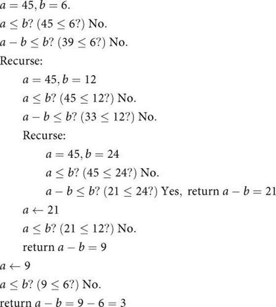
Remember that since the Greeks had no notion of a zero-length segment, their remainders were in the range [1, n].
We still have the overhead of recursion, so we’ll eventually want to come up with an iterative solution, but we’ll put that aside for now.
Finally, we can plug this code into our GCM function, providing a solution to Exercise 4.1:
line_segment fast_segment_gcm(line_segment a, line_segment b) {
while (a != b) {
a = fast_segment_remainder(a, b);
std::swap(a, b);
}
return a;
}
Of course, no matter how fast it is, this code will still never terminate if a and b do not have a common measure.
4.3 A Millennium without Mathematics
As we have seen, ancient Greece was a source of several centuries of astonishing mathematical developments. By the 3rd century BC, mathematics was a flourishing field of study, with Archimedes (best known today for a story about discovering the principle of buoyancy in his bathtub) its most dominant figure. Unfortunately, the rise of Roman power led to a stagnation in Western mathematics that would last for almost 1500 years. While the Romans built great works of engineering, they were generally uninterested in advancing the mathematics that made these structures possible. As the great Roman statesman Cicero said in his Tusculan Disputations:
Among the Greeks geometry was held in highest honor; nothing could outshine mathematics. But we have limited the usefulness of this art to measuring and calculating.
While there were Greek mathematicians working in Roman times, it is a remarkable fact that there is no record of any original mathematical text written in Latin (the language of ancient Rome) at that time.
The period of history that followed was not kind to the formerly great societies of Europe. In Byzantium, the Greek-speaking Eastern remnant of the former Roman Empire, mathematics was still studied, but innovation declined. By the 6th to 7th centuries, scholars still read Euclid, but usually just the first book of Elements; Latin translations didn’t even bother to include the proofs. By the end of the first millennium, if you were a European who wanted to study mathematics, you had to go to cities like Cairo, Baghdad, or Cordoba in the realm of the Arabs.
Other Mathematical Traditions
Throughout ancient times, mathematics developed in many parts of the world. Civilization depends on mathematics. All major civilizations developed number systems, which were a fundamental requirement for two critical civic activities: collecting taxes and computing calendars to determine cultivation dates.
Furthermore, all major civilizations developed common mathematical concepts, such as Pythagorean triples (sets of three integers a, b, c where a2+b2 = c2). While some have argued that this implies a common Neolithic source of mathematical knowledge that spread throughout the world, there is no evidence for this claim. Today it seems more likely that this is simply the mathematical equivalent of convergent evolution in biology, where the same characteristics evolve independently in unrelated species. The fact that these same mathematical ideas were rediscovered independently suggests their fundamental nature.
Many civilizations developed important mathematical traditions at some point in their history. For example, in China, 3rd-century mathematician and poet Liu Hui wrote important commentaries on an earlier book, Nine Chapters on the Mathematical Art, and extended the work. Among other discoveries, he demonstrated that the value of π must be greater than 3, and provided several geometric techniques for surveying. In India, 5th-century mathematician and astronomer Aryabhata wrote a foundational text called the Aryabhatiya, which included algorithms for computing square and cube roots, as well as geometric techniques. Ideas of Indian mathematics were further developed by Arab, Persian, and Jewish scholars, all writing in Arabic, who in turn heavily influenced the rebirth of European mathematics in the early 13th century.
Computer science emerged from this reinvigorated European mathematics, so this is what we are focusing on. As programmers, we are all heirs of this tradition.
4.4 The Strange History of Zero
The next development in the history of Euclid’s algorithm required something the Greeks didn’t have: zero. You may have heard that ancient societies had no notion of zero, and that it was invented by Indians or Arabs, but this is only partially correct. In fact, Babylonian astronomers were using zero as early as 1500 BC, together with a positional number system. However, their number system used base 60. The rest of their society used base 10—for example, in commerce—without either zero or positional notation. Amazingly, this state of affairs persisted for centuries. Greek astronomers eventually learned the Babylonian system and used it (still in base 60) for their trigonometric computations, but again, this approach was used only for this one application and was unknown to the rest of society. (It was also these Greek astronomers who started using the Greek letter omicron, which looks just like our letter “O,” to represent zero.)
What is particularly surprising about the lack of zero outside of astronomy is that it persisted despite the fact that the abacus was well known and commonly used for commerce in nearly every ancient civilization. Abaci consist of stones or beads arranged in columns; the columns correspond to 1s, 10s, 100s, and so on, and each bead represents one unit of a given power of 10. In other words, ancient societies used a device that represented numbers in base 10 positional notation, yet there was no commonly used written representation of zero until 1000 years later.
The unification of a written form of zero with a decimal positional notation is due to early Indian mathematicians sometime around the 6th century AD. It then spread to Persia between the 6th and 9th centuries AD. Arab scholars learned the technique and spread it across their empire, from Baghdad in the east to Cordoba in the west. There is no evidence that zero was known anywhere in Europe outside this empire (even in the rest of Spain); 300 years would pass before this innovation crossed from one culture to the other.
The breakthrough came in 1203 when Leonardo Pisano, also known as Fibonacci, published Liber Abaci (“The Book of Calculation”). In addition to introducing zero and positional decimal notation, this astonishing book described to Europeans, for the first time, the standard algorithms for doing arithmetic that we are now taught in elementary school: long addition, long subtraction, long multiplication, and long division. With one stroke, Leonardo brought mathematics back to Europe.
Leonardo Pisano (1170–ca. 1240)
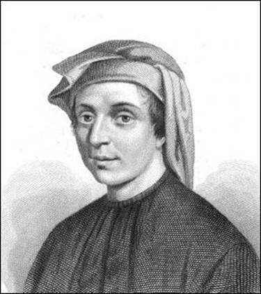
The Italian city of Pisa, which today is landlocked, was a major port and naval power in the 12th and 13th century. It competed with Venice as the dominant trading center in the Mediterranean. Thousands of Pisan traders crisscrossed the sea routes to the Middle East, Byzantium, North Africa, and Spain, and the Pisan government sent trade representatives to major cities to ensure their success. One of these representatives, Guglielmo Bonacci, was posted to Algeria. He decided to bring his son Leonardo along, a decision that changed the course of mathematical history.
Leonardo learned “Hindu digits” from the Arabs, and continued his studies during business trips to Egypt, Syria, Sicily, Greece, and Provence. In his book Liber Abaci, he would go on to introduce their innovations (including zero) to Europe. But Liber Abaci was not just a translation of other people’s work: it was a first-class mathematical treatise with many fundamental new contributions. Leonardo would go on to write several more books on various branches of mathematics, including some of the most important mathematical developments in centuries.
He called himself Leonardo Pisano (“Leonardo the Pisan”), although since the 19th century he has usually been known as Fibonacci, an abbreviation of filius Bonacci (“son of Bonacci”).
Leonardo’s fame reached the Holy Roman Emperor, Frederick II, a great intellectual conversant in many languages and a patron of science and mathematics, whose court was in Palermo, Sicily. Frederick came to Pisa and organized a challenge to Leonardo by his court mathematicians. Leonardo performed well and impressed the visiting dignitaries. Toward the end of his life, the city of Pisa gave him a salary as a reward for his great contributions.
Leonardo Pisano’s later work Liber Quadratorum (“The Book of Squares”), published in 1225, is probably the greatest work on number theory in the time span between Diophantus 1000 years earlier and the great French mathematician Pierre de Fermat 400 years later. Here is one of the problems from the book:
Exercise 4.3 (easy). Prove that ![]() .
.
Why was a problem like this difficult for the Greeks? They had no terminating procedure for computing cube roots (in fact, it was later proven that no such process exists). So from their perspective, the problem starts out: “First, execute a nonterminating procedure....”
Leonardo’s insight will be familiar to any middle-school algebra student, but it was revolutionary in the 13th century. Basically, what he said was, “Even though I don’t know how to compute ![]() , I’ll just pretend I do and assign it an arbitrary symbol.”
, I’ll just pretend I do and assign it an arbitrary symbol.”
Here’s another example of the kind of problem Leonardo solved:
Exercise 4.4. Prove the following proposition from Liber Quadratorum: For any odd square number x, there is an even square number y, such that x + y is a square number.
Exercise 4.5 (hard). Prove the following proposition from Liber Quadratorum: If x and y are both sums of two squares, then so is their product xy. (This is an important result that Fermat builds on.)
4.5 Remainder and Quotient Algorithms
Once zero was widely used in mathematics, it actually took centuries longer before it occurred to anyone that a segment could have zero length—specifically, the segment ![]() .
.
Zero-length segments force us to rethink our GCM and remainder procedures, because Archimedes’ axiom no longer holds—we can add a zero-length segment forever, and we’ll never exceed a nonzero segment. So we’ll allow the first argument a to be zero, but we need a precondition to ensure that the second argument b is not zero. Having zero also lets us shift our remainders to the range [0, n – 1], which will be crucial for modular arithmetic and other developments. Here’s the code:
line_segment fast_segment_remainder1(line_segment a,
line_segment b) {
// precondition: b != 0
if (a < b) return a;
if (a - b < b) return a - b;
a = fast_segment_remainder1(a, b + b);
if (a < b) return a;
return a - b;
}
The only thing we’ve changed are the conditions; everywhere we used to say a <= b, we now check a < b.
Let’s see if we can get rid of the recursion. Every time we recurse down, we double b, so in the iterative version, we’d like to precompute the maximum amount of doubling we’ll need. We can define a function that finds the first repeated doubling of b that exceeds the difference a – b:
line_segment largest_doubling(line_segment a, line_segment b) {
// precondition: b != 0
while (a - b >= b) b = b + b;
return b;
}
Now we need our iterative function to do the same computation that happens on the way out of the recursion. Each time it returns, the value of b has the value it had before the most recent recursive call (i.e., the most recent doubling). So to simulate this, the iterative version needs to repeatedly “undouble” the value, which it will do by calling a function half. Remember, we’re still “computing” with ruler and compass. Fortunately, there is a Euclidean procedure for “halving” a segment,1 so we can use a half function. Now we can write an iterative version of remainder:
line_segment remainder(line_segment a, line_segment b) {
// precondition: b != 0
if (a < b) return a;
line_segment c = largest_doubling(a, b);
a = a - c;
while (c != b) {
c = half(c);
if (c <= a) a = a - c;
}
return a;
}
1 Draw a circle with the center at one end of the segment and radius equal to the segment; repeat for the other end. Use ruler to connect the two points where the circles intersect. The resulting line will bisect the original segment.
The first part of the function, which finds the largest doubling value, does what the “downward” recursion does, while the last part does what happens on the way back up out of the recursive calls. Let’s look again at our example of finding the remainder of 45 divided by 6, this time with the new remainder function:
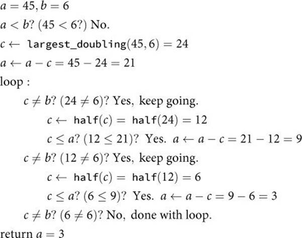
Notice that the successive values of c in the iterative implementation are the same as the values of b following each recursive call in the recursive implementation. Also, compare this to the trace of our earlier version of the algorithm at the end of Section 4.2. Observe how the results of the first part (c = 24 and a = 21) here are the same as the innermost recursion in the old example.
This is an extremely efficient algorithm, nearly as fast as the hardware implemented remainder operation in modern processors.
* * *
What if we wanted to compute quotient instead of remainder? It turns out that the code is almost the same. All we need are a couple of minor modifications, shown in bold:
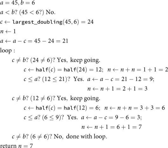
integer quotient(line_segment a, line_segment b) {
// Precondition: b > 0
if (a < b) return integer(0);
line_segment c = largest_doubling(a, b);
integer n(1);
a = a - c;
while (c != b) {
c = half(c); n = n + n;
if (c <= a) { a = a - c; n = n + 1; }
}
return n;
}
Quotient is the number of times one line segment fits into another, so we use the type integer to represent this count. Basically, we are going to count multiples of b. If a < b, then we don’t have any multiples of b and we return 0. But if a ≥ b, we initialize the counter to 1, then double it each time we halve c, adding one more multiple for each iteration when it fits. Again, let’s work through an example. This time, instead of finding the remainder of 45 divided by 6, we’ll find the quotient of 45 divided by 6.
Essentially, this is the Egyptian multiplication algorithm in reverse. And Ahmes knew it: a primitive variant of this algorithm, known to the Greeks as Egyptian division, appears in the Rhind papyrus.
4.6 Sharing the Code
Since the majority of the code is shared between quotient and remainder, it would make much more sense to combine them into a single function that returns both values; the complexity of the combined function is the same as either individual function. Note that C++11 allows us to use initializer list syntax {x, y} to construct the pair that the function returns:
std::pair<integer, line_segment>
quotient_remainder(line_segment a, line_segment b) {
// Precondition: b > 0
if (a < b) return {integer(0), a};
line_segment c = largest_doubling(a, b);
integer n(1);
a = a - c;
while (c != b) {
c = half(c); n = n + n;
if (c <= a) { a = a - c; n = n + 1; }
}
return {n, a};
}
In fact, any quotient or remainder function does nearly all the work of the other.
Programming Principle: The Law of Useful Return
Our quotient_remainder function illustrates an important programming principle, which we call the law of useful return:
If you’ve already done the work to get some useful result, don’t throw it away. Return it to the caller.
This may allow the caller to get some extra work done “for free” (as in the quotient_remainder case) or to return data that can be used in future invocations of the function.
Unfortunately, this principle is not always followed. For example, the C and C++ programming languages have separate quotient and remainder operators; there is no way for a programmer to get both results with one call—despite the fact that many processors have an instruction that returns both.
Most computing architectures, whether ruler-and-compass or modern CPUs, provide an easy way to compute half; for us, it’s just a 1-bit right shift. However, if you should happen to be working with an architecture that doesn’t support this functionality, there is a remarkable version of the remainder function developed by Robert Floyd and Donald Knuth that does not require halving. It’s based on the idea of the Fibonacci sequence—another of Leonardo Pisano’s inventions, which we will discuss more in Chapter 7. Instead of the next number being double the previous one, we’ll make the next number be the sum of the two previous ones:2
line_segment remainder_fibonacci(line_segment a, line_segment b) {
// Precondition: b > 0
if (a < b) return a;
line_segment c = b;
do {
line_segment tmp = c; c = b + c; b = tmp;
} while (a >= c);
do {
if (a >= b) a = a - b;
line_segment tmp = c - b; c = b; b = tmp;
} while (b < c);
return a;
}
2 Note that this sequence starts at b, so the values will not be the same as the traditional Fibonacci sequence.
The first loop is equivalent to computing largest_doubling in our previous algorithm. The second loop corresponds to the “halving” part of the code. But instead of halving, we use subtraction to get back the earlier number in the Fibonacci sequence. This works because we always keep one previous value around in a temporary variable.
Exercise 4.6. Trace the remainder_fibonacci algorithm as it computes the remainder of 45 and 6, in the way we traced the remainder algorithm in Section 4.5.
Exercise 4.7. Design quotient_fibonacci and quotient_remainder_fibonacci.
Now that we have an efficient implementation of the remainder function, we can return to our original problem, the greatest common measure. Using our new remainder function from p. 54, we can rewrite Euclid’s algorithm like this:
line_segment gcm_remainder(line_segment a, line_segment b) {
while (b != line_segment(0)) {
a = remainder(a, b);
std::swap(a, b);
}
return a;
}
Since we now allow remainder to return zero, the termination condition for the main loop is when b (the previous iteration’s remainder) is zero, instead of comparing a and b as we did originally.
We will use this algorithm for the next few chapters, leaving its structure intact but exploring how it applies to different types. We will leave our ruler-and-compass constructions behind and implement the algorithm with a digital computer in mind. For example, for integers, the equivalent function is the greatest common divisor (GCD):
integer gcd(integer a, integer b) {
while (b != integer(0)) {
a = a % b;
std::swap(a, b);
}
return a;
}
The code is identical, except that we have replaced line_segment with integer and used the modulus operator % to compute the remainder. Since computers have instructions to compute the integer remainder (as invoked by the C++ modulus operator), it’s better to use them than to rely on doubling and halving.
4.7 Validating the Algorithm
How do we know that the integer GCD algorithm works? We need to show two things: first, that the algorithm terminates, and second, that it computes the GCD.
To prove that the algorithm terminates, we rely on the fact that
0 ≤ (a mod b) < b
Therefore, in each iteration, the remainder gets smaller. Since any decreasing sequence of positive integers is finite, the algorithm must terminate.
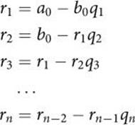
To prove that the algorithm computes the GCD, we start by observing that in each iteration, the algorithm computes a remainder of a and b, which by definition is
r = a – bq
where q is the integer quotient of a divided by b. Since gcd(a, b) by definition divides a and also divides b (and therefore bq), it must also divide r. We can rewrite the remainder equation as follows:
a = bq + r
By the same reasoning, since gcd(b, r) by definition divides b (and therefore bq), and also divides r, it must also divide a. Since pairs (a, b) and (b, r) have the same common divisors, they have the same greatest common divisor. Therefore we have shown that
![]()
At each iteration, the algorithm replaces gcd(a, b) with gcd(b, r) by taking the remainder and swapping the arguments. Here is the list of remainders, starting with a0 and b0, the initial arguments to the function:
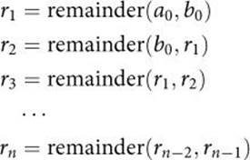
Using the definition of remainder, we rewrite the sequence computed by the algorithm like this:
What Equation 4.1 guarantees is that the GCD stays the same each time. In other words:
gcd(a0, b0) = gcd(b0, r1) = gcd(r1, r2) = ··· = gcd(rn–1, rn)
But we know that the remainder of rn-1 and rn is 0, because that’s what triggers the termination of the algorithm. And gcd(x, 0) = x. So
gcd(a0, b0) = ··· = gcd(rn–1, rn) = gcd(rn, 0) = rn
which is the value returned by the algorithm. Therefore, the algorithm computes the GCD of its original arguments.
4.8 Thoughts on the Chapter
We’ve seen how an ancient algorithm for computing the greatest common measure of two line segments could be turned into a modern function for computing the GCD of integers. We’ve looked at variants of the algorithm and seen its relationship to functions for finding the quotient and the remainder. Does the GCD algorithm work for other things besides line segments and integers? In other words, is there a way to make the algorithm more general? We’ll come back to that question later in the book.