OpenGL ES 3.0: Programming Guide, Second Edition (2014)
Chapter 14. Advanced Programming with OpenGL ES 3.0
In this chapter, we put together many of the techniques you have learned throughout this book to discuss some advanced uses of OpenGL ES 3.0. A large number of advanced rendering techniques can be accomplished with the programmable flexibility of OpenGL ES 3.0. In this chapter, we cover the following techniques:
• Per-fragment lighting
• Environment mapping
• Particle system with point sprites
• Particle system with transform feedback
• Image postprocessing
• Projective texturing
• Noise using a 3D texture
• Procedural textures
• Terrain rendering with vertex texture fetch
• Shadows using a depth texture
Per-Fragment Lighting
In Chapter 8, “Vertex Shaders,” we covered the lighting equations that can be used in the vertex shader to calculate per-vertex lighting. Commonly, to achieve higher-quality lighting, we seek to evaluate the lighting equations on a per-fragment basis. In this section, we provide an example of evaluating ambient, diffuse, and specular lighting on a per-fragment basis. This example is a PVRShaman workspace that can be found in Chapter_14/PVR_PerFragmentLighting, as pictured in Figure 14-1. Several of the examples in this chapter make use of PVRShaman, a shader development integrated development environment (IDE) that is part of the Imagination Technologies PowerVR SDK (downloadable from http://powervrinsider.com/).
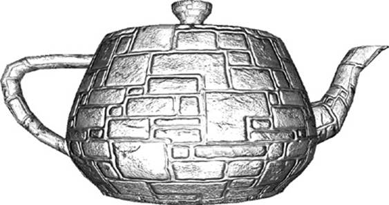
Figure 14-1 Per-Fragment Lighting Example
Lighting with a Normal Map
Before we get into the details of the shaders used in the PVRShaman workspace, we need to discuss the general approach that is used in the example. The simplest way to do lighting per-fragment would be to use the interpolated vertex normal in the fragment shader and then move the lighting computations into the fragment shader. However, for the diffuse term, this would really not yield much better results than doing the lighting on a per-vertex basis. There would be the advantage that the normal vector could be renormalized, which would remove artifacts due to linear interpolation, but the overall quality would be only minimally better. To really take advantage of the ability to do computations on a per-fragment basis, we need to use a normal map to store per-texel normals—a technique that can provide significantly more detail.
A normal map is a 2D texture that stores a normal vector at each texel. The red channel represents the x component, the green channel the y component, and the blue channel the z component. For a normal map stored as GL_RGB8 with GL_UNSIGNED_BYTE data, the values will all be in the range [0, 1]. To represent a normal, these values need to be scaled and biased in the shader to remap to [−1, 1]. The following block of fragment shader code shows how you would go about fetching from a normal map:
// Fetch the tangent space normal from normal map
vec3 normal = texture(s_bumpMap, v_texcoord).xyz;
// Scale and bias from [0, 1] to [−1, 1] and normalize
normal = normalize(normal * 2.0 − 1.0);
As you can see, this small bit of shader code will fetch the color value from a texture map and then multiply the results by 2 and subtract 1. The result is that the values are rescaled into the [−1, 1] range from the [0, 1] range. We could actually avoid this scale and bias in the shader code by using a signed texture format such as GL_RGB8_SNORM, but for the purposes of demonstration we are showing how to use a normal map stored in an unsigned format. In addition, if the data in your normal map are not normalized, you will need to normalize the results in the fragment shader. This step can be skipped if your normal map contains all unit vectors.
The other significant issue to tackle with per-fragment lighting has to do with the space in which the normals in the texture are stored. To minimize computations in the fragment shader, we do not want to have to transform the result of the normal fetched from the normal map. One way to accomplish this would be to store world-space normals in your normal map. That is, the normal vectors in the normal map would each represent a world-space normal vector. Then, the light and direction vectors could be transformed into world space in the vertex shader and could be directly used with the value fetched from the normal map. However, some significant issues arise when storing normal maps in world space. Most importantly, the object must be assumed to be static because no transformation can happen on the object. In addition, the same surface oriented in different directions in space would not be able to share the same texels in the normal map, which can result in much larger maps.
A better solution than using world-space normal maps is to store normal maps in tangent space. The idea behind tangent space is that we define a space for each vertex using three coordinate axes: the normal, binormal, and tangent. The normals stored in the texture map are then all stored in this tangent space. Then, when we want to compute any lighting equations, we transform our incoming lighting vectors into the tangent space and those light vectors can then be used directly with the values in the normal map. The tangent space is typically computed as a preprocess and the binormal and tangent are added to the vertex attribute data. This work is done automatically by PVRShaman, which computes a tangent space for any model that has a vertex normal and texture coordinates.
Lighting Shaders
Once we have tangent space normal maps and tangent space vectors set up, we can proceed with per-fragment lighting. First, let’s look at the vertex shader in Example 14-1.
Example 14-1 Per-Fragment Lighting Vertex Shader
#version 300 es
uniform mat4 u_matViewInverse;
uniform mat4 u_matViewProjection;
uniform vec3 u_lightPosition;
uniform vec3 u_eyePosition;
in vec4 a_vertex;
in vec2 a_texcoord0;
in vec3 a_normal;
in vec3 a_binormal;
in vec3 a_tangent;
out vec2 v_texcoord;
out vec3 v_viewDirection;
out vec3 v_lightDirection;
void main( void )
{
// Transform eye vector into world space
vec3 eyePositionWorld =
(u_matViewInverse * vec4(u_eyePosition, 1.0)).xyz;
// Compute world−space direction vector
vec3 viewDirectionWorld = eyePositionWorld − a_vertex.xyz;
// Transform light position into world space
vec3 lightPositionWorld =
(u_matViewInverse * vec4(u_lightPosition, 1.0)).xyz;
// Compute world−space light direction vector
vec3 lightDirectionWorld = lightPositionWorld − a_vertex.xyz;
// Create the tangent matrix
mat3 tangentMat = mat3( a_tangent,
a_binormal,
a_normal );
// Transform the view and light vectors into tangent space
v_viewDirection = viewDirectionWorld * tangentMat;
v_lightDirection = lightDirectionWorld * tangentMat;
// Transform output position
gl_Position = u_matViewProjection * a_vertex;
// Pass through texture coordinate
v_texcoord = a_texcoord0.xy;
}
Note that the vertex shader inputs and uniforms are set up automatically by PVRShaman by setting semantics in the PerFragmentLighting.pfx file. We have two uniform matrices that we need as input to the vertex shader: u_matViewInverse and u_matViewProjection. Theu_matViewInverse matrix contains the inverse of the view matrix. This matrix is used to transform the light vector and the eye vector (which are in view space) into world space. The first four statements in main perform this transformation and compute the light vector and view vector in world space. The next step in the shader is to create a tangent matrix. The tangent space for the vertex is stored in three vertex attributes: a_normal, a_binormal, and a_tangent. These three vectors define the three coordinate axes of the tangent space for each vertex. We construct a 3 × 3 matrix out of these vectors to form the tangent matrix tangentMat.
The next step is to transform the view and direction vectors into tangent space by multiplying them by the tangentMat matrix. Remember, our purpose here is to get the view and direction vectors into the same space as the normals in the tangent-space normal map. By doing this transformation in the vertex shader, we avoid performing any transformations in the fragment shader. Finally, we compute the final output position and place it in gl_Position and pass the texture coordinate along to the fragment shader in v_texcoord.
Now we have the view and direction vector in view space and a texture coordinate passed as out variables to the fragment shader. The next step is to actually light the fragments using the fragment shader, as shown in Example 14-2.
Example 14-2 Per-Fragment Lighting Fragment Shader
#version 300 es
precision mediump float;
uniform vec4 u_ambient;
uniform vec4 u_specular;
uniform vec4 u_diffuse;
uniform float u_specularPower;
uniform sampler2D s_baseMap;
uniform sampler2D s_bumpMap;
in vec2 v_texcoord;
in vec3 v_viewDirection;
in vec3 v_lightDirection;
layout(location = 0) out vec4 fragColor;
void main( void )
{
// Fetch base map color
vec4 baseColor = texture(s_baseMap, v_texcoord);
// Fetch the tangent space normal from normal map
vec3 normal = texture(s_bumpMap, v_texcoord).xyz;
// Scale and bias from [0, 1] to [−1, 1] and
// normalize
normal = normalize(normal * 2.0 − 1.0);
// Normalize the light direction and view
// direction
vec3 lightDirection = normalize(v_lightDirection);
vec3 viewDirection = normalize(v_viewDirection);
// Compute N.L
float nDotL = dot(normal, lightDirection);
// Compute reflection vector
vec3 reflection = (2.0 * normal * nDotL) −
lightDirection;
// Compute R.V
float rDotV =
max(0.0, dot(reflection, viewDirection));
// Compute ambient term
vec4 ambient = u_ambient * baseColor;
// Compute diffuse term
vec4 diffuse = u_diffuse * nDotL * baseColor;
// Compute specular term
vec4 specular = u_specular *
pow(rDotV, u_specularPower);
// Output final color
fragColor = ambient + diffuse + specular;
}
The first part of the fragment shader consists of a series of uniform declarations for the ambient, diffuse, and specular colors. These values are stored in the uniform variables u_ambient, u_diffuse, and u_specular, respectively. The shader is also configured with two samplers,s_baseMap and s_bumpMap, which are bound to a base color map and the normal map, respectively.
The first part of the fragment shader fetches the base color from the base map and the normal values from the normal map. As described earlier, the normal vector fetched from the texture map is scaled and biased and then normalized so that it is a unit vector with components in the [−1, 1] range. Next, the light vector and view vector are normalized and stored in lightDirection and viewDirection. Normalization is necessary because of the way fragment shader input variables are interpolated across a primitive. The fragment shader input variables are linearly interpolated across the primitive. When linear interpolation is done between two vectors, the results can become denormalized during interpolation. To compensate for this artifact, the vectors must be normalized in the fragment shader.
Lighting Equations
At this point in the fragment shader, we now have a normal, light vector, and direction vector all normalized and in the same space. This gives us the inputs needed to compute the lighting equations. The lighting computations performed in this shader are as follows:
Ambient = kAmbient × CBase
Diffuse = kDiffuse × N • L × CBase
Specular = kSpecular × pow(max(R • V, 0.0), kSpecular Power
The k constants for ambient, diffuse, and specular colors come from the u_ambient, u_diffuse, and u_specular uniform variables. The CBase is the base color fetched from the base texture map. The dot product of the light vector and the normal vector, N • L, is computed and stored in the nDotL variable in the shader. This value is used to compute the diffuse lighting term. Finally, the specular computation requires R, which is the reflection vector computed from the equation
R = 2 × N × (N • L) − L
Notice that the reflection vector also requires N • L, so the computation used for the diffuse lighting term can be reused in the reflection vector computation. Finally, the lighting terms are stored in the ambient, diffuse, and specular variables in the shader. These results are summedand finally stored in the fragColor output variable. The result is a per-fragment lit object with normal data coming from the normal map.
Many variations are possible on per-fragment lighting. One common technique is to store the specular exponent in a texture along with a specular mask value. This allows the specular lighting to vary across a surface. The main purpose of this example is to give you an idea of the types of computations that are typically done for per-fragment lighting. The use of tangent space, along with the computation of the lighting equations in the fragment shader, is typical of many modern games. Of course, it is also possible to add more lights, more material information, and much more.
Environment Mapping
The next rendering technique we cover—related to the previous technique—is performing environment mapping using a cubemap. The example we cover is the PVRShaman workspace Chapter_14/PVR_EnvironmentMapping. The results are shown in Figure 14-2.
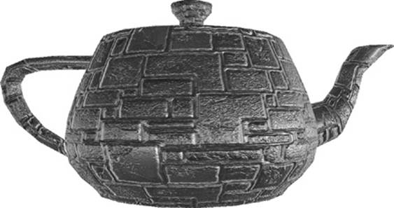
Figure 14-2 Environment Mapping Example
The concept behind environment mapping is to render the reflection of the environment on an object. In Chapter 9, “Texturing,” we introduced cubemaps, which are commonly used to store environment maps. In the PVRShaman example workspace, the environment of a mountain scene is stored in a cubemap. The way such cubemaps can be generated is by positioning a camera at the center of a scene and rendering along each of the positive and negative major axis directions using a 90-degree field of view. For reflections that change dynamically, we can render such a cubemap using a framebuffer object dynamically for each frame. For a static environment, this process can be done as a preprocess and the results stored in a static cubemap.
The vertex shader for the environment mapping example is provided in Example 14-3.
Example 14-3 Environment Mapping Vertex Shader
#version 300 es
uniform mat4 u_matViewInverse;
uniform mat4 u_matViewProjection;
uniform vec3 u_lightPosition;
in vec4 a_vertex;
in vec2 a_texcoord0;
in vec3 a_normal;
in vec3 a_binormal;
in vec3 a_tangent;
out vec2 v_texcoord;
out vec3 v_lightDirection;
out vec3 v_normal;
out vec3 v_binormal;
out vec3 v_tangent;
void main( void )
{
// Transform light position into world space
vec3 lightPositionWorld =
(u_matViewInverse * vec4(u_lightPosition, 1.0)).xyz;
// Compute world−space light direction vector
vec3 lightDirectionWorld = lightPositionWorld − a_vertex.xyz;
// Pass the world−space light vector to the fragment shader
v_lightDirection = lightDirectionWorld;
// Transform output position
gl_Position = u_matViewProjection * a_vertex;
// Pass through other attributes
v_texcoord = a_texcoord0.xy;
v_normal = a_normal;
v_binormal = a_binormal;
v_tangent = a_tangent;
}
The vertex shader in this example is very similar to the previous per-fragment lighting example. The primary difference is that rather than transforming the light direction vector into tangent space, we keep the light vector in world space. The reason we must do this is because we ultimately want to fetch from the cubemap using a world-space reflection vector. As such, rather than transforming the light vectors into tangent space, we will transform the normal vector from tangent space into world space. To do so, the vertex shader passes the normal, binormal, and tangent as varyings into the fragment shader so that a tangent matrix can be constructed.
The fragment shader listing for the environment mapping sample is provided in Example 14-4.
Example 14-4 Environment Mapping Fragment Shader
#version 300 es
precision mediump float;
uniform vec4 u_ambient;
uniform vec4 u_specular;
uniform vec4 u_diffuse;
uniform float u_specularPower;
uniform sampler2D s_baseMap;
uniform sampler2D s_bumpMap;
uniform samplerCube s_envMap;
in vec2 v_texcoord;
in vec3 v_lightDirection;
in vec3 v_normal;
in vec3 v_binormal;
in vec3 v_tangent;
layout(location = 0) out vec4 fragColor;
void main( void )
{
// Fetch base map color
vec4 baseColor = texture( s_baseMap, v_texcoord );
// Fetch the tangent space normal from normal map
vec3 normal = texture( s_bumpMap, v_texcoord ).xyz;
// Scale and bias from [0, 1] to [−1, 1]
normal = normal * 2.0 − 1.0;
// Construct a matrix to transform from tangent to
// world space
mat3 tangentToWorldMat = mat3( v_tangent,
v_binormal,
v_normal );
// Transform normal to world space and normalize
normal = normalize( tangentToWorldMat * normal );
// Normalize the light direction
vec3 lightDirection = normalize( v_lightDirection );
// Compute N.L
float nDotL = dot( normal, lightDirection );
// Compute reflection vector
vec3 reflection = ( 2.0 * normal * nDotL ) − lightDirection;
// Use the reflection vector to fetch from the environment
// map
vec4 envColor = texture( s_envMap, reflection );
// Output final color
fragColor = 0.25 * baseColor + envColor;
}
In the fragment shader, you will notice that the normal vector is fetched from the normal map in the same way as in the per-fragment lighting example. The difference in this example is that rather than leaving the normal vector in tangent space, the fragment shader transforms the normal vector into world space. This is done by constructing the tangentToWorld matrix out of the v_tangent, v_binormal, and v_normal varying vectors and then multiplying the fetched normal vector by this new matrix. The reflection vector is then calculated using the light direction vector and normal, both in world space. The result of the computation is a reflection vector that is in world space, exactly what we need to fetch from the cubemap as an environment map. This vector is used to fetch into the environment map using the texture function with thereflection vector as a texture coordinate. Finally, the resultant fragColor is written as a combination of the base map color and the environment map color. The base color is attenuated by 0.25 for the purposes of this example so that the environment map is clearly visible.
This example demonstrates the basics of environment mapping. The same basic technique can be used to produce a large variety of effects. For example, the reflection may be attenuated using a fresnel term to more accurately model the reflection of light on a given material. As mentioned earlier, another common technique is to dynamically render a scene into a cubemap so that the environment reflection varies as an object moves through a scene and the scene itself changes. Using the basic technique shown here, you can extend the technique to accomplish more advanced reflection effects.
Particle System with Point Sprites
The next example we cover is rendering a particle explosion using point sprites. This example demonstrates how to animate a particle in a vertex shader and how to render particles using point sprites. The example we cover is the sample program in Chapter_14/ParticleSystem, the results of which are pictured in Figure 14-3.
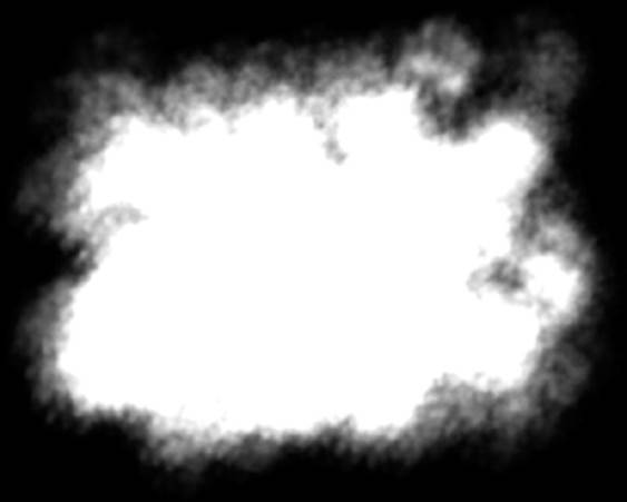
Figure 14-3 Particle System Sample
Particle System Setup
Before diving into the code for this example, it’s helpful to cover at a high level the approach this sample uses. One of the goals here is to show how to render a particle explosion without having any dynamic vertex data modified by the CPU. That is, with the exception of uniform variables, there are no changes to any of the vertex data as the explosion animates. To accomplish this goal, a number of inputs are fed into the shaders.
At initialization time, the program initializes the following values in a vertex array, one for each particle, based on a random value:
• Lifetime—The lifetime of a particle in seconds.
• Start position—The start position of a particle in the explosion.
• End position—The final position of a particle in the explosion (the particles are animated by linearly interpolating between the start and end position).
In addition, each explosion has several global settings that are passed in as uniforms:
• Center position—The center of the explosion (the per-vertex positions are offset from this center).
• Color—An overall color for the explosion.
• Time—The current time in seconds.
Particle System Vertex Shader
With this information, the vertex and fragment shaders are completely responsible for the motion, fading, and rendering of the particles. Let’s begin by looking at the vertex shader code for the sample in Example 14-5.
Example 14-5 Particle System Vertex Shader
#version 300 es
uniform float u_time;
uniform vec3 u_centerPosition;
layout(location = 0) in float a_lifetime;
layout(location = 1) in vec3 a_startPosition;
layout(location = 2) in vec3 a_endPosition;
out float v_lifetime;
void main()
{
if ( u_time <= a_lifetime )
{
gl_Position.xyz = a_startPosition +
(u_time * a_endPosition);
gl_Position.xyz += u_centerPosition;
gl_Position.w = 1.0;
}
else
{
gl_Position = vec4( −1000, −1000, 0, 0 );
}
v_lifetime = 1.0 − ( u_time / a_lifetime );
v_lifetime = clamp ( v_lifetime, 0.0, 1.0 );
gl_PointSize = ( v_lifetime * v_lifetime ) * 40.0;
}
The first input to the vertex shader is the uniform variable u_time. This variable is set to the current elapsed time in seconds by the application. The value is reset to 0.0 when the time exceeds the length of a single explosion. The next input to the vertex shader is the uniform variableu_centerPosition. This variable is set to the center location of the explosion at the start of a new explosion. The setup code for u_time and u_centerPosition appears in the Update function in the C code of the example program, which is provided in Example 14-6.
Example 14-6 Update Function for Particle System Sample
void Update (ESContext *esContext, float deltaTime)
{
UserData *userData = esContext−>userData;
userData−>time += deltaTime;
glUseProgram ( userData−>programObject );
if(userData−>time >= l.Of)
{
float centerPos[3];
float color[4] ;
userData−>time = O.Of;
// Pick a new start location and color
centerPos[0] = ((float)(rand() % 10000)/10000.0f)−0.5f;
centerPos[l] = ((float)(rand() % 10000)/10000.0f)−0.5f;
centerPos[2] = ((float)(rand() % 10000)/10000.0f)−0.5f;
glUniform3fv(userData−>centerPositionLoc, 1,
¢erPos[0]);
// Random color
color[0] = ((float)(rand() % 10000) / 20000.Of) + 0.5f;
color[l] = ((float)(rand() % 10000) / 20000.Of) + 0.5f;
color[2] = ((float)(rand() % 10000) / 20000.Of) + 0.5f;
color[3] = 0.5;
glUniform4fv(userData−>colorLoc, 1, &color[0]);
}
// Load uniform time variable
glUniformlf(userData−>timeLoc, userData−>time);
}
As you can see, the Update function resets the time after 1 second elapses and then sets up a new center location and time for another explosion. The function also keeps the u_time variable up-to-date in each frame.
The vertex inputs to the vertex shader are the particle lifetime, particle start position, and end position. These variables are all initialized to randomly seeded values in the Init function in the program. The body of the vertex shader first checks whether a particle’s lifetime has expired. If so, the gl_Position variable is set to the value (−1000, −1000), which is just a quick way of forcing the point to be off the screen. Because the point will be clipped, all of the subsequent processing for the expired point sprites can be skipped. If the particle is still alive, its position is set to be a linear interpolated value between the start and end positions. Next, the vertex shader passes the remaining lifetime of the particle down into the fragment shader in the varying variable v_lifetime. The lifetime will be used in the fragment shader to fade the particle as it ends its life. The final piece of the vertex shader causes the point size to be based on the remaining lifetime of the particle by setting the gl_Pointsize built-in variable. This has the effect of scaling the particles down as they reach the end of their life.
Particle System Fragment Shader
The fragment shader code for the example program is provided in Example 14-7.
Example 14-7 Particle System Fragment Shader
#version 300 es
precision mediump float;
uniform vec4 u_color;
in float v_lifetime;
layout(location = 0) out vec4 fragColor;
uniform sampler2D s_texture;
void main()
{
vec4 texColor;
texColor = texture( s_texture, gl_PointCoord );
fragColor = vec4( u_color ) * texColor;
fragColor.a *= v_lifetime;
}
The first input to the fragment shader is the u_color uniform variable, which is set at the beginning of each explosion by the Update function. Next, the v_lifetime input variable set by the vertex shader is declared in the fragment shader. In addition, a sampler is declared to which a 2D texture image of smoke is bound.
The fragment shader itself is relatively simple. The texture fetch uses the gl_PointCoord variable as a texture coordinate. This special variable for point sprites is set to fixed values for the corners of the point sprite (this process was described in Chapter 7, “Primitive Assembly and Rasterization,” in the discussion of drawing primitives). One could also extend the fragment shader to rotate the point sprite coordinates if rotation of the sprite was required. This requires extra fragment shader instructions, but increases the flexibility of the point sprite.
The texture color is attenuated by the u_color variable, and the alpha value is attenuated by the particle lifetime. The application also enables alpha blending with the following blend function:
glEnable ( GL_BLEND );
glBlendFunc ( GL_SRC_ALPHA, GL_ONE );
As a consequence of this code, the alpha produced in the fragment shader is modulated with the fragment color. This value is then added into whatever values are stored in the destination of the fragment. The result is an additive blend effect for the particle system. Note that various particle effects will use different alpha blending modes to accomplish the desired effect.
The code to actually draw the particles is shown in Example 14-8.
Example 14-8 Draw Function for Particle System Sample
void Draw ( ESContext *esContext )
{
UserData *userData = esContext−>userData;
// Set the viewport
glViewport ( 0, 0, esContext−>width, esContext−>height );
// Clear the color buffer
glClear ( GL_COLOR_BUFFER_BIT );
// Use the program object
glUseProgram ( userData−>programObject );
// Load the vertex attributes
glVertexAttribPointer ( ATTRIBUTE_LIFETIME_LOC, 1,
GL_FLOAT, GL_FALSE,
PARTICLE_SIZE * sizeof(GLfloat),
userData−>particleData );
glVertexAttribPointer ( ATTRIBUTE_ENDPOSITION_LOC, 3,
GL_FLOAT, GL_FALSE,
PARTICLE_SIZE * sizeof(GLfloat),
&userData−>particleData[1] );
glVertexAttribPointer ( ATTRIBUTE_STARTPOSITION_LOC, 3,
GL_FLOAT, GL_FALSE,
PARTICLE_SIZE * sizeof(GLfloat),
&userData−>particleData[4] );
glEnableVertexAttribArray ( ATTRIBUTE_LIFETIME_LOC );
glEnableVertexAttribArray ( ATTRIBUTE_ENDPOSITION_LOC );
glEnableVertexAttribArray ( ATTRIBUTE_STARTPOSITION_LOC );
// Blend particles
glEnable ( GL_BLEND );
glBlendFunc ( GL_SRC_ALPHA, GL_ONE );
// Bind the texture
glActiveTexture ( GL_TEXTURE0 );
glBindTexture ( GL_TEXTURE_2D, userData−>textureId );
// Set the sampler texture unit to 0
glUniform1i ( userData−>samplerLoc, 0 );
glDrawArrays( GL_POINTS, 0, NUM_PARTICLES );
}
The Draw function begins by setting the viewport and clearing the screen. It then selects the program object to use and loads the vertex data using glVertexAttribPointer. Note that because the values of the vertex array never change, this example could have used vertex buffer objects rather than client-side vertex arrays. In general, this approach is recommended for any vertex data that does not change because it reduces the vertex bandwidth used. Vertex buffer objects were not used in this example merely to keep the code a bit simpler. After setting the vertex arrays, the function enables the blend function, binds the smoke texture, and then uses glDrawArrays to draw the particles.
Unlike with triangles, there is no connectivity for point sprites, so using glDrawElements does not really provide any advantage for rendering point sprites in this example. However, often particle systems need to be sorted by depth from back to front to achieve proper alpha blending results. In such cases, one potential approach is to sort the element array to modify the draw order. This technique is very efficient, because it requires minimal bandwidth across the bus per frame (only the index data need be changed, and they are almost always smaller than the vertex data).
This example has demonstrated a number of techniques that can be useful in rendering particle systems using point sprites. The particles were animated entirely on the GPU using the vertex shader. The sizes of the particles were attenuated based on particle lifetime using thegl_PointSize variable. In addition, the point sprites were rendered with a texture using the gl_PointCoord built-in texture coordinate variable. These are the fundamental elements needed to implement a particle system using OpenGL ES 3.0.
Particle System Using Transform Feedback
The previous example demonstrated one technique for animating a particle system in the vertex shader. Although it included an efficient method for animating particles, the result was severely limited compared to a traditional particle system. In a typical CPU-based particle system, particles are emitted with different initial parameters such as position, velocity, and acceleration and the paths are animated over the particle’s lifetime. In the previous example, all of the particles were emitted simultaneously and the paths were limited to a linear interpolation between the start and end positions.
We can build a much more general-purpose GPU-based particle system by using the transform feedback feature of OpenGL ES 3.0. To review, transform feedback allows the outputs of the vertex shader to be stored in a buffer object. As a consequence, we can implement a particle emitter completely in a vertex shader on the GPU, store its output into a buffer object, and then use that buffer object with another shader to draw the particles. In general, transform feedback allows you to implement render to vertex buffer (sometimes referred to by the shorthand R2VB), which means that a wide range of algorithms can be moved from the CPU to the GPU.
The example we cover in this section is found in Chapter_14/ParticleSystemTransformFeedback. It demonstrates emitting particles for a fountain using transform feedback, as shown in Figure 14-4.

Figure 14-4 Particle System with Transform Feedback
Particle System Rendering Algorithm
This section provides a high-level overview of how the transform feedback-based particle system works. At initialization time, two buffer objects are allocated to hold the particle data. The algorithm ping-pongs (switches back and forth) between the two buffers, each time switching which buffer is the input or output for particle emission. Each particle contains the following information: position, velocity, size, current time, and lifetime.
The particle system is updated with transform feedback and then rendered in the following steps:
• In each frame, one of the particle VBOs is selected as the input and bound as a GL_ARRAY_BUFFER. The output is bound as a GL_TRANSFORM_FEEDBACK_BUFFER.
• GL_RASTERIZER_DISCARD is enabled so that no fragments are drawn.
• The particle emission shader is executed using point primitives (each particle is one point). The vertex shader outputs new particles to the transform feedback buffer and copies existing particles to the transform feedback buffer unchanged.
• GL_RASTERIZER_DISCARD is disabled, so that the application can draw the particles.
• The buffer that was rendered to for transform feedback is now bound as a GL_ARRAY_BUFFER. Another vertex/fragment shader is bound to draw the particles.
• The particles are rendered to the framebuffer.
• In the next frame, the input/output buffer objects are swapped and the same process continues.
Particle Emission with Transform Feedback
Example 14-9 shows the vertex shader that is used for emitting particles. All of the output variables in this shader are written to a transform feedback buffer object. Whenever a particle’s lifetime has expired, the shader will make it a potential candidate for emission as a new active particle. If a new particle is generated, the shader uses a randomValue function (shown in the vertex shader code in Example 14-9) that generates a random value to initialize the new particle’s velocity and size. The random number generation is based on using a 3D noise texture and using thegl_VertexID built-in variable to select a unique texture coordinate for each particle. The details of creating and using a 3D Noise texture are described in the Noise Using a 3D Texture section later in this chapter.
Example 14-9 Particle Emission Vertex Shader
#version 300 es
#define NUM_PARTICLES 200
#define ATTRIBUTE_POSITION 0
#define ATTRIBUTE_VELOCITY 1
#define ATTRIBUTE_SIZE 2
#define ATTRIBUTE_CURTIME 3
#define ATTRIBUTE_LIFETIME 4
uniform float u_time;
uniform float u_emissionRate;
uniform sampler3D s_noiseTex;
layout(location = ATTRIBUTE_POSITION) in vec2 a_position;
layout(location = ATTRIBUTE_VELOCITY) in vec2 a_velocity;
layout(location = ATTRIBUTE_SIZE) in float a_size;
layout(location = ATTRIBUTE_CURTIME) in float a_curtime;
layout(location = ATTRIBUTE_LIFETIME) in float a_lifetime;
out vec2 v_position;
out vec2 v_velocity;
out float v_size;
out float v_curtime;
out float v_lifetime;
float randomValue( inout float seed )
{
float vertexId = float( gl_VertexID ) /
float( NUM_PARTICLES );
vec3 texCoord = vec3( u_time, vertexId, seed );
seed += 0.1;
return texture( s_noiseTex, texCoord ).r;
}
void main()
{
float seed = u_time;
float lifetime = a_curtime − u_time;
if( lifetime <= 0.0 && randomValue(seed) < u_emissionRate )
{
// Generate a new particle seeded with random values for
// velocity and size
v_position = vec2( 0.0, −1.0 );
v_velocity = vec2( randomValue(seed) * 2.0 − 1.00,
randomValue(seed) * 0.4 + 2.0 );
v_size = randomValue(seed) * 20.0 + 60.0;
v_curtime = u_time;
v_lifetime = 2.0;
}
else
{
// This particle has not changed; just copy it to the
// output
v_position = a_position;
v_velocity = a_velocity;
v_size = a_size;
v_curtime = a_curtime;
v_lifetime = a_lifetime;
}
}
To use the transform feedback feature with this vertex shader, the output variables must be tagged as being used for transform feedback before linking the program object. This is done in the InitEmitParticles function in the example code, where the following snippet shows how the program object is set up for transform feedback:
char* feedbackVaryings[5] =
{
"v_position",
"v_velocity",
"v_size",
"v_curtime",
"v_lifetime"
};
// Set the vertex shader outputs as transform
// feedback varyings
glTransformFeedbackVaryings ( userData−>emitProgramObject, 5,
feedbackVaryings,
GL_INTERLEAVED_ATTRIBS );
// Link program must occur after calling
// glTransformFeedbackVaryings
glLinkProgram( userData−>emitProgramObject );
The call to glTransformFeedbackVaryings ensures that the passed-in output variables are used for transform feedback. The GL_INTERLEAVED_ATTRIBS parameter specifies that the output variables will be interleaved in the output buffer object. The order and layout of the variables must match the expected layout of the buffer object. In this case, our vertex structure is defined as follows:
typedef struct
{
float position[2];
float velocity[2];
float size;
float curtime;
float lifetime;
} Particle;
This structure definition matches the order and type of the varyings that are passed in to glTransformFeedbackVaryings.
The code used to emit the particles is provided in the EmitParticles function shown in Example 14-10.
Example 14-10 Emit Particles with Transform Feedback
void EmitParticles ( ESContext *esContext, float deltaTime )
{
UserData userData = (UserData) esContext−>userData;
GLuint srcVBO =
userData−>particleVBOs[ userData−>curSrcIndex ];
GLuint dstVBO =
userData−>particleVBOs[(userData−>curSrcIndex+1) % 2];
glUseProgram( userData−>emitProgramObject );
// glVertexAttribPointer and glEnableVeretxAttribArray
// setup
SetupVertexAttributes(esContext, srcVBO);
// Set transform feedback buffer
glBindBufferBase(GL_TRANSFORM_FEEDBACK_BUFFER, 0, dstVBO);
// Turn off rasterization; we are not drawing
glEnable(GL_RASTERIZER_DISCARD);
// Set uniforms
glUniform1f(userData−>emitTimeLoc, userData−>time);
glUniform1f(userData−>emitEmissionRateLoc, EMISSION_RATE);
// Bind the 3D noise texture
glActiveTexture(GL_TEXTURE0);
glBindTexture(GL_TEXTURE_3D, userData−>noiseTextureId);
glUniform1i(userData−>emitNoiseSamplerLoc, 0);
// Emit particles using transform feedback
glBeginTransformFeedback(GL_POINTS);
glDrawArrays(GL_POINTS, 0, NUM_PARTICLES);
glEndTransformFeedback();
// Create a sync object to ensure transform feedback
// results are completed before the draw that uses them
userData−>emitSync = glFenceSync(
GL_SYNC_GPU_COMMANDS_COMPLETE, 0 );
// Restore state
glDisable(GL_RASTERIZER_DISCARD);
glUseProgram(0);
glBindBufferBase(GL_TRANSFORM_FEEDBACK_BUFFER, 0, 0);
glBindTexture(GL_TEXTURE_3D, 0);
// Ping−pong the buffers
userData−>curSrcIndex = ( userData−>curSrcIndex + 1 ) % 2;
}
The destination buffer object is bound to the GL_TRANSFORM_FEEDBACK_BUFFER target using glBindBufferBase. Rasterization is disabled by enabling GL_RASTERIZER_DISCARD because we will not actually draw any fragments; instead, we simply want to execute the vertex shader and output to the transform feedback buffer. Finally, before the glDrawArrays call, we enable transform feedback rendering by calling glBeginTransformFeedback(GL_POINTS). Subsequent calls to glDrawArrays using GL_POINTS will then be recorded in the transform feedback buffer until glEndTransformFeedback is called. To ensure transform feedback results are completed before the draw call that uses them, we create a sync object and insert a fence command immediately after the glEndTransformFeedback is called. Prior to the draw call execution, we will wait on the sync object using the glWaitSync call. After executing the draw call and restoring state, we ping-pong between the buffers so that the next time EmitShaders is called, it will use the previous frame’s transform feedback output as the input.
Rendering the Particles
After emitting the transform feedback buffer, that buffer is bound as a vertex buffer object from which to render the particles. The vertex shader used for particle rendering with point sprites is provided in Example 14-11.
Example 14-11 Particle Rendering Vertex Shader
#version 300 es
#define ATTRIBUTE_POSITION 0
#define ATTRIBUTE_VELOCITY 1
#define ATTRIBUTE_SIZE 2
#define ATTRIBUTE_CURTIME 3
#define ATTRIBUTE_LIFETIME 4
layout(location = ATTRIBUTE_POSITION) in vec2 a_position;
layout(location = ATTRIBUTE_VELOCITY) in vec2 a_velocity;
layout(location = ATTRIBUTE_SIZE) in float a_size;
layout(location = ATTRIBUTE_CURTIME) in float a_curtime;
layout(location = ATTRIBUTE_LIFETIME) in float a_lifetime;
uniform float u_time;
uniform vec2 u_acceleration;
void main()
{
float deltaTime = u_time − a_curtime;
if ( deltaTime <= a_lifetime )
{
vec2 velocity = a_velocity + deltaTime * u_acceleration;
vec2 position = a_position + deltaTime * velocity;
gl_Position = vec4( position, 0.0, 1.0 );
gl_PointSize = a_size * ( 1.0 − deltaTime / a_lifetime );
}
else
{
gl_Position = vec4( −1000, −1000, 0, 0 );
gl_PointSize = 0.0;
}
}
This vertex shader uses the transform feedback outputs as input variables. The current age of each particle is computed based on the timestamp that was stored at particle creation for each particle in the a_curtime attribute. The particle’s velocity and position are updated based on this time. Additionally, the size of the particle is attenuated over the particle’s life.
This example has demonstrated how to generate and render a particle system entirely on the GPU. While the particle emitter and rendering were relatively simple here, the same basic model can be used to create more complex particle systems with more involved physics and properties. The primary takeaway message is that transform feedback allows us to generate new vertex data on the GPU without the need for any CPU code. This powerful feature can be used for many algorithms that require generating vertex data on the GPU.
Image Postprocessing
The next example covered in this chapter involves image postprocessing. Using a combination of framebuffer objects and shaders, it is possible to perform a wide variety of image postprocessing techniques. The first example presented here is the simple blur effect in the PVRShaman workspace in Chapter_14/PVR_PostProcess, results of which are pictured in Figure 14-5.
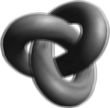
Figure 14-5 Image Postprocessing Example
Render-to-Texture Setup
This example renders a textured knot into a framebuffer object and then uses the color attachment as a texture in a subsequent pass. A full-screen quad is drawn to the screen using the rendered texture as a source. A fragment shader is run over the full-screen quad, which performs a blur filter. In general, many types of postprocessing techniques can be accomplished using this pattern:
1. Render the scene into an off-screen framebuffer object (FBO).
2. Bind the FBO texture as a source and render a full-screen quad to the screen.
3. Execute a fragment shader that performs filtering across the quad.
Some algorithms require performing multiple passes over an image; others require more complicated inputs. However, the general idea is to use a fragment shader over a full-screen quad that performs a postprocessing algorithm.
Blur Fragment Shader
The fragment shader used on the full-screen quad in the blurring example is provided in Example 14-12.
Example 14-12 Blur Fragment Shader
#version 300 es
precision mediump float;
uniform sampler2D renderTexture;
uniform float u_blurStep;
in vec2 v_texCoord;
layout(location = 0) out vec4 outColor;
void main(void)
{
vec4 sample0,
sample1,
sample2,
sample3;
float fStep = u_blurStep / 100.0;
sample0 = texture2D ( renderTexture,
vec2 ( v_texCoord.x − fStep, v_texCoord.y − fStep ) );
sample1 = texture2D ( renderTexture,
vec2 ( v_texCoord.x + fStep, v_texCoord.y + fStep ) );
sample2 = texture2D ( renderTexture,
vec2 ( v_texCoord.x + fStep, v_texCoord.y − fStep ) );
sample3 = texture2D ( renderTexture,
vec2 ( v_texCoord.x − fStep, v_texCoord.y + fStep) );
outColor = (sample0 + sample1 + sample2 + sample3) / 4.0;
}
This shader begins by computing the fStep variable, which is based on the u_blurstep uniform variable. The fStep variable is used to determine how much to offset the texture coordinate when fetching samples from the image. A total of four different samples are taken from the image and then averaged together at the end of the shader. The fStep variable is used to offset the texture coordinate in four directions such that four samples in each diagonal direction from the center are taken. The larger the value of fStep, the more the image is blurred. One possible optimization to this shader would be to compute the offset texture coordinates in the vertex shader and pass them into varyings in the fragment shader. This approach would reduce the amount of computation done per fragment.
Light Bloom
Now that we have looked at a simple image postprocessing technique, let’s consider a slightly more complicated one. Using the blurring technique we introduced in the previous example, we can implement an effect known as light bloom. Light bloom is what happens when the eye views a bright light contrasted with a darker surface—that is, the light color bleeds into the darker surface. As you can see from the screenshot in Figure 14-6, the car model color bleeds over the background. The algorithm works as follows:
1. Clear an off-screen render target (rt0) and draw the object in black.
2. Blur the off-screen render target (rt0) into another render target (rtl) using a blur step of 1.0.
3. Blur the off-screen render target (rt1) back into the original render target (rt0) using a blur step of 2.0.
Note
For more blur, repeat steps 2 and 3 for the amount of blur, increasing the blur step each time.
4. Render the object to the back buffer.
5. Blend the final render target with the back buffer.
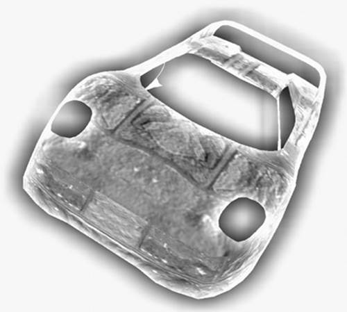
Figure 14-6 Light Bloom Effect
The process this algorithm uses is illustrated in Figure 14-7, which shows each of the steps that goes into producing the final image. As you can see in this figure, the object is first rendered in black to the render target. That render target is then blurred into a second render target in the next pass. The blurred render target is then blurred again, with an expanded blur kernel going back into the original render target. At the end, that blurred render target is blended with the original scene. The amount of bloom can be increased by ping-ponging the blur targets over and over. The shader code for the blur steps is the same as in the previous example; the only difference is that the blur step is being increased for each pass.
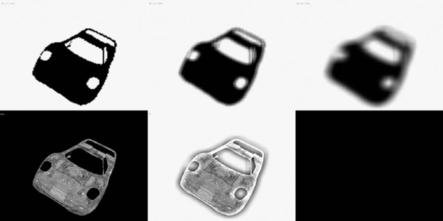
Figure 14-7 Light Bloom Stages
A large variety of other image postprocessing algorithms can be performed using a combination of FBOs and shaders. Some other common techniques include tone mapping, selective blurring, distortion, screen transitions, and depth of field. Using the techniques shown here, you can start to implement other postprocessing algorithms using shaders.
Projective Texturing
A technique that is used to produce many effects, such as shadow mapping and reflections, is projective texturing. To introduce the topic of projective texturing, we provide an example of rendering a projective spotlight. Most of the complexity in using projective texturing derives from the mathematics that goes into calculating the projective texture coordinates. The method shown here could also be used to produce texture coordinates for shadow mapping or reflections. The example offered here is found in the projective spotlight PVRShaman workspace inChapter_14/PVR_ProjectiveSpotlight, the results of which are pictured in Figure 14-8.
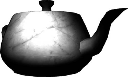
Figure 14-8 Projective Spotlight Example
Projective Texturing Basics
The example uses the 2D texture image pictured in Figure 14-9 and applies it to the surface of a teapot using projective texturing. Projective spotlights were a very common technique used to emulate per-pixel spotlight falloff before shaders were introduced to GPUs. Projective spotlights can still provide an attractive solution because of their high level of efficiency. Applying the projective texture takes just a single texture fetch instruction in the fragment shader and some setup in the vertex shader. In addition, the 2D texture image that is projected can contain really any picture, so many different effects can be achieved.
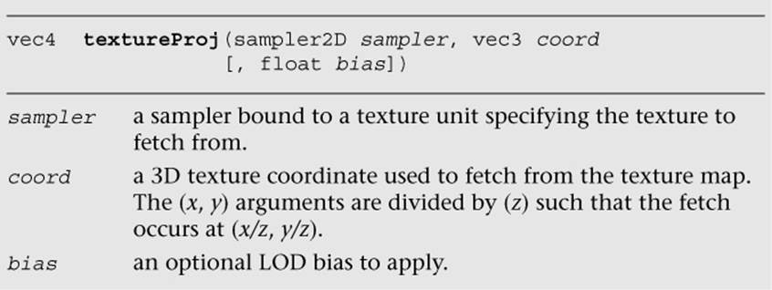

Figure 14-9 2D Texture Projected onto Object
What, exactly, do we mean by projective texturing? At its most basic, projective texturing is the use of a 3D texture coordinate to look up into a 2D texture image. The (s, t) coordinates are divided by the (r) coordinate such that a texel is fetched using (s/r, t/r). The OpenGL ES Shading Language provides a special built-in function to do projective texturing called textureProj.
The idea behind projective lighting is to transform the position of an object into the projective view space of a light. The projective light space position, after application of a scale and bias, can then be used as a projective texture coordinate. The vertex shader in the PVRShaman example workspace does the work of transforming the position into the projective view space of a light.
Matrices for Projective Texturing
There are three matrices that we need to transform the position into projective view space of the light and get a projective texture coordinate:
• Light projection—projection matrix of the light source using the field of view, aspect ratio, and near and far planes of the light.
• Light view—The view matrix of the light source. This would be constructed just as if the light were a camera.
• Bias matrix—A matrix that transforms the light-space projected position into a 3D projective texture coordinate.
The light projection matrix would be constructed just like any other projection matrix, using the light’s parameters for field of view (FOV), aspect ratio (aspect), and near (zNear) and far plane (zFar) distances.
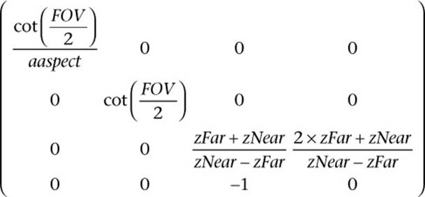
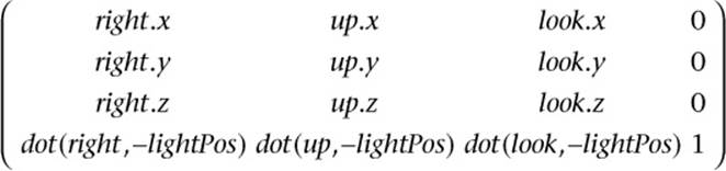
The light view matrix is constructed by using the three primary axis directions that define the light’s view axes and the light’s position. We refer to the axes as the right, up, and look vectors.
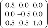
After transforming the object’s position by the view and projection matrices, we must then turn the coordinates into projective texture coordinates. This is accomplished by using a 3 × 3 bias matrix on the (x, y, z) components of the position in projective light space. The bias matrix does a linear transformation to go from the [−1, 1] range to the [0, 1] range. Having the coordinates in the [0, 1] range is necessary for the values to be used as texture coordinates.
Typically, the matrix to transform the position into a projective texture coordinate would be computed on the CPU by concatenating the projection, view, and bias matrices together (using a 4 × 4 version of the bias matrix). The result would then be loaded into a single uniform matrix that could transform the position in the vertex shader. However, in the example, we perform this computation in the vertex shader for illustrative purposes.
Projective Spotlight Shaders
Now that we have covered the basic mathematics, we can examine the vertex shader in Example 14-13.
Example 14-13 Projective Texturing Vertex Shader
#version 300 es
uniform float u_time_0_X;
uniform mat4 u_matProjection;
uniform mat4 u_matViewProjection;
in vec4 a_vertex;
in vec2 a_texCoord0;
in vec3 a_normal;
out vec2 v_texCoord;
out vec3 v_projTexCoord;
out vec3 v_normal;
out vec3 v_lightDir;
void main( void )
{
gl_Position = u_matViewProjection * a_vertex;
v_texCoord = a_texCoord0.xy;
// Compute a light position based on time
vec3 lightPos;
lightPos.x = cos(u_time_0_X);
lightPos.z = sin(u_time_0_X);
lightPos.xz = 200.0 * normalize(lightPos.xz);
lightPos.y = 200.0;
// Compute the light coordinate axes
vec3 look = −normalize( lightPos );
vec3 right = cross( vec3( 0.0, 0.0, 1.0), look );
vec3 up = cross( look, right );
// Create a view matrix for the light
mat4 lightView = mat4( right, dot( right, −lightPos ),
up, dot( up, −lightPos ),
look, dot( look, −lightPos),
0.0, 0.0, 0.0, 1.0 );
// Transform position into light view space
vec4 objPosLight = a_vertex * lightView;
// Transform position into projective light view space
objPosLight = u_matProjection * objPosLight;
// Create bias matrix
mat3 biasMatrix = mat3( 0.5, 0.0, 0.5,
0.0, −0.5, 0.5,
0.0, 0.0, 1.0 );
// Compute projective texture coordinates
v_projTexCoord = objPosLight.xyz * biasMatrix;
v_lightDir = normalize(a_vertex.xyz − lightPos);
v_normal = a_normal;
}
The first operation this shader does is to transform the position by the u_matViewProjection matrix and output the texture coordinate for the base map to the v_texCoord output variable. Next, the shader computes a position for the light based on time. This bit of the code can really be ignored, but it was added to animate the light in the vertex shader. In a typical application, this step would be done on the CPU and not in the shader.
Based on the position of the light, the vertex shader then computes the three coordinate axis vectors for the light and places the results into the look, right, and up variables. Those vectors are used to create a view matrix for the light in the lightView variable using the equations previously described. The input position for the object is then transformed by the lightView matrix, which transforms the position into light space. The next step is to use the perspective matrix to transform the light space position into projected light space. Rather than creating a new perspective matrix for the light, this example uses the u_matProjection matrix for the camera. Typically, a real application would want to create its own projection matrix for the light based on how big the cone angle and falloff distance are.
Once the position is transformed into projective light space, a biasMatrix is created to transform the position into a projective texture coordinate. The final projective texture coordinate is stored in the vec3 output variable v_projTexCoord. In addition, the vertex shader passes the light direction and normal vectors into the fragment shader in the v_lightDir and v_normal variables. These vectors will be used to determine whether a fragment is facing the light source so as to mask off the projective texture for fragments facing away from the light.
The fragment shader performs the actual projective texture fetch that applies the projective spotlight texture to the surface (Example 14-14).
Example 14-14 Projective Texturing Fragment Shader
#version 300 es
precision mediump float;
uniform sampler2D baseMap;
uniform sampler2D spotLight;
in vec2 v_texCoord;
in vec3 v_projTexCoord;
in vec3 v_normal;
in vec3 v_lightDir;
out vec4 outColor;
void main( void )
{
// Projective fetch of spotlight
vec4 spotLightColor =
textureProj( spotLight, v_projTexCoord );
// Base map
vec4 baseColor = texture( baseMap, v_texCoord );
// Compute N.L
float nDotL = max( 0.0, −dot( v_normal, v_lightDir ) );
outColor = spotLightColor * baseColor * 2.0 * nDotL;
}
The first operation that the fragment shader performs is the projective texture fetch using textureProj. As you can see, the projective texture coordinate that was computed during the vertex shader and passed in the input variable v_projTexCoord is used to perform the projective texture fetch. The wrap modes for the projective texture are set to GL_CLAMP_TO_EDGE and the minification/magnification filters are both set to GL_LINEAR. The fragment shader then fetches the color from the base map using the v_texCoord variable. Next, the shader computes the dot product of the light direction and the normal vector; this result is used to attenuate the final color so that the projective spotlight is not applied to fragments that are facing away from the light. Finally, all of the components are multiplied together (and scaled by 2.0 to increase the brightness). This gives us the final image of the teapot lit by the projective spotlight (refer back to Figure 14-7).
As mentioned at the beginning of this section, the key takeaway lesson from this example is the set of computations that go into computing a projective texture coordinate. The computation shown here is the exact same computation that you would use to produce a coordinate to fetch from a shadow map. Similarly, rendering reflections with projective texturing requires that you transform the position into the projective view space of the reflection camera. You would do the same thing we have done here, but substitute the light matrices for the reflection camera matrices. Projective texturing is a very powerful tool in creating advanced effects, and you should now understand the basics of how to use it.
Noise Using a 3D Texture
The next rendering technique we cover is using a 3D texture for noise. In Chapter 9, “Texturing,” we introduced the basics of 3D textures. As you will recall, a 3D texture is essentially a stack of 2D texture slices representing a 3D volume. 3D textures have many possible uses, one of which is the representation of noise. In this section, we show an example of using a 3D volume of noise to create a wispy fog effect. This example builds on the linear fog example from Chapter 10, “Fragment Shaders.” The example is found in Chapter_14/Noise3D, the results of which are shown in Figure 14-10.

Figure 14-10 Fog Distorted by 3D Noise Texture
Generating Noise
The application of noise is a very common technique that plays a role in a large variety of 3D effects. The OpenGL Shading Language (not OpenGL ES Shading Language) included functions for computing noise in one, two, three, and four dimensions. These functions return a pseudorandom continuous noise value that is repeatable based on the input value. Unfortunately, the functions are expensive to implement. Most programmable GPUs did not implement noise functions natively in hardware, which meant the noise computations had to be implemented using shader instructions (or worse, in software on the CPU). It takes a lot of shader instructions to implement these noise functions, so the performance was too slow to be used in most real-time fragment shaders. Recognizing this problem, the OpenGL ES working group decided to drop noise from the OpenGL ES Shading Language (although vendors are still free to expose it through an extension).
Although computing noise in the fragment shader is prohibitively expensive, we can work around the problem using a 3D texture. It is possible to easily produce acceptable-quality noise by precomputing the noise and placing the results in a 3D texture. A number of algorithms can be used to generate noise. The list of references and links described at the end of this chapter can be used to obtain more information about the various noise algorithms. Here, we discuss a specific algorithm that generates a lattice-based gradient noise. Ken Perlin’s noise function (Perlin, 1985) is a lattice-based gradient noise and a widely used method for generating noise. For example, a lattice-based gradient noise is implemented by the noise function in the Renderman shading language.
The gradient noise algorithm takes a 3D coordinate as input and returns a floating-point noise value. To generate this noise value given an input (x, y, z), we map the x, y, and z values to appropriate integer locations in a lattice. The number of cells in a lattice is programmable and for our implementation is set to 256 cells. For each cell in the lattice, we need to generate and store a pseudorandom gradient vector. Example 14-15 describes how these gradient vectors are generated.
Example 14-15 Generating Gradient Vectors
// permTable describes a random permutation of
// 8−bit values from 0 to 255
static unsigned char permTable[256] = {
0xE1, 0x9B, 0xD2, 0x6C, 0xAF, 0xC7, 0xDD, 0x90,
0xCB, 0x74, 0x46, 0xD5, 0x45, 0x9E, 0x21, 0xFC,
0x05, 0x52, 0xAD, 0x85, 0xDE, 0x8B, 0xAE, 0x1B,
0x09, 0x47, 0x5A, 0xF6, 0x4B, 0x82, 0x5B, 0xBF,
0xA9, 0x8A, 0x02, 0x97, 0xC2, 0xEB, 0x51, 0x07,
0x19, 0x71, 0xE4, 0x9F, 0xCD, 0xFD, 0x86, 0x8E,
0xF8, 0x41, 0xE0, 0xD9, 0x16, 0x79, 0xE5, 0x3F,
0x59, 0x67, 0x60, 0x68, 0x9C, 0x11, 0xC9, 0x81,
0x24, 0x08, 0xA5, 0x6E, 0xED, 0x75, 0xE7, 0x38,
0x84, 0xD3, 0x98, 0x14, 0xB5, 0x6F, 0xEF, 0xDA,
0xAA, 0xA3, 0x33, 0xAC, 0x9D, 0x2F, 0x50, 0xD4,
0xB0, 0xFA, 0x57, 0x31, 0x63, 0xF2, 0x88, 0xBD,
0xA2, 0x73, 0x2C, 0x2B, 0x7C, 0x5E, 0x96, 0x10,
0x8D, 0xF7, 0x20, 0x0A, 0xC6, 0xDF, 0xFF, 0x48,
0x35, 0x83, 0x54, 0x39, 0xDC, 0xC5, 0x3A, 0x32,
0xD0, 0x0B, 0xF1, 0x1C, 0x03, 0xC0, 0x3E, 0xCA,
0x12, 0xD7, 0x99, 0x18, 0x4C, 0x29, 0x0F, 0xB3,
0x27, 0x2E, 0x37, 0x06, 0x80, 0xA7, 0x17, 0xBC,
0x6A, 0x22, 0xBB, 0x8C, 0xA4, 0x49, 0x70, 0xB6,
0xF4, 0xC3, 0xE3, 0x0D, 0x23, 0x4D, 0xC4, 0xB9,
0x1A, 0xC8, 0xE2, 0x77, 0x1F, 0x7B, 0xA8, 0x7D,
0xF9, 0x44, 0xB7, 0xE6, 0xB1, 0x87, 0xA0, 0xB4,
0x0C, 0x01, 0xF3, 0x94, 0x66, 0xA6, 0x26, 0xEE,
0xFB, 0x25, 0xF0, 0x7E, 0x40, 0x4A, 0xA1, 0x28,
0xB8, 0x95, 0xAB, 0xB2, 0x65, 0x42, 0x1D, 0x3B,
0x92, 0x3D, 0xFE, 0x6B, 0x2A, 0x56, 0x9A, 0x04,
0xEC, 0xE8, 0x78, 0x15, 0xE9, 0xD1, 0x2D, 0x62,
0xC1, 0x72, 0x4E, 0x13, 0xCE, 0x0E, 0x76, 0x7F,
0x30, 0x4F, 0x93, 0x55, 0x1E, 0xCF, 0xDB, 0x36,
0x58, 0xEA, 0xBE, 0x7A, 0x5F, 0x43, 0x8F, 0x6D,
0x89, 0xD6, 0x91, 0x5D, 0x5C, 0x64, 0xF5, 0x00,
0xD8, 0xBA, 0x3C, 0x53, 0x69, 0x61, 0xCC, 0x34,
};
#define NOISE_TABLE_MASK 255
// lattice gradients 3D noise
static float gradientTable[256*3];
#define FLOOR(x) ((int)(x) − ((x) < 0 && (x) != (int)(x)))
#define smoothstep(t) (t * t * (3.0f − 2.0f * t))
#define lerp(t, a, b) (a + t * (b − a))
void initNoiseTable()
{
int i;
float a;
float x, y, z, r, theta;
float gradients[256*3];
unsigned int *p, *psrc;
srandom(0);
// build gradient table for 3D noise
for (i=0; i<256; i++)
{
/*
* calculate 1 − 2 * random number
*/
a = (random() % 32768) / 32768.0f;
z = (1.0f − 2.0f * a);
r = sqrtf(1.0f − z * z); // r is radius of circle
a = (random() % 32768) / 32768.0f;
theta = (2.0f * (float)M_PI * a);
x = (r * cosf(a));
y = (r * sinf(a));
gradients[i*3] = x;
gradients[i*3+1] = y;
gradients[i*3+2] = z;
}
// use the index in the permutation table to load the
// gradient values from gradients to gradientTable
p = (unsigned int *)gradientTable;
psrc = (unsigned int *)gradients;
for (i=0; i<256; i++)
{
int indx = permTable[i];
p[i*3] = psrc[indx*3];
p[i*3+1] = psrc[indx*3+1];
p[i*3+2] = psrc[indx*3+2];
}
}
Example 14-16 shows how the gradient noise is calculated using the pseudorandom gradient vectors and an input 3D coordinate.
Example 14-16 3D Noise
//
// generate the value of gradient noise for a given lattice
// point
//
// (ix, iy, iz) specifies the 3D lattice position
// (fx, fy, fz) specifies the fractional part
//
static float
glattice3D(int ix, int iy, int iz, float fx, float fy,
float fz)
{
float *g;
int indx, y, z;
z = permTable[iz & NOISE_TABLE_MASK];
y = permTable[(iy + z) & NOISE_TABLE_MASK];
indx = (ix + y) & NOISE_TABLE_MASK;
g = &gradientTable[indx*3];
return (g[0]*fx + g[l]*fy + g[2]*fz);
}
//
// generate the 3D noise value
// f describes input (x, y, z) position for which the noise value
// needs to be computed. noise3D returns the scalar noise value
//
float
noise3D(float *f)
{
int ix, iy, iz;
float fxO, fxl, fyO, fyl, fzO, fzl;
float wx, wy, wz;
float vxO, vxl, vyO, vyl, vzO, vzl;
ix = FLOOR(f[0]);
fxO = f[0] − ix;
fxl = fxO − 1;
wx = smoothstep(fxO);
iy = FLOOR(f[1]);
fyO = f[1] − iy;
fyl = fyO − 1;
wy = smoothstep(fyO);
iz = FLOOR(f[2]);
fzO = f[2] − iz;
fzl = fzO − 1;
wz = smoothstep(fzO);
vxO = glattice3D(ix, iy, iz, fxO, fyO, fzO);
vxl = glattice3D(ix+1, iy, iz, fxl, fyO, fzO);
vyO = lerp(wx, vxO, vxl);
vxO = glattice3D(ix, iy+1, iz, fxO, fyl, fzO);
vxl = glattice3D(ix+1, iy+1, iz, fxl, fyl, fzO);
vyl = lerp(wx, vxO, vxl);
vzO = lerp(wy, vyO, vyl);
vxO = glattice3D(ix, iy, iz+1, fxO, fyO, fzl);
vxl = glattice3D(ix+1, iy, iz+1, fxl, fyO, fzl);
vyO = lerp(wx, vxO, vxl);
vxO = glattice3D(ix, iy+1, iz+1, fxO, fyl, fzl);
vxl = glattice3D(ix+1, iy+1, iz+1, fxl, fyl, fzl);
vyl = lerp(wx, vxO, vxl);
vzl = lerp(wy, vyO, vyl);
return lerp(wz, vzO, vzl);;
}
The noise3D function returns a value between −1.0 and 1.0. The value of gradient noise is always 0 at the integer lattice points. For points in between, trilinear interpolation of gradient values across the eight integer lattice points that surround the point is used to generate the scalar noisevalue. Figure 14-11 shows a 2D slice of the gradient noise using the preceding algorithm.
Figure 14-11 2D Slice of Gradient Noise
Using Noise
Once we have created a 3D noise volume, it is very easy to use it to produce a variety of effects. In the case of the wispy fog effect, the idea is simple: Scroll the 3D noise texture in all three dimensions based on time and use the value from the texture to distort the fog factor. Let’s take a look at the fragment shader in Example 14-17.
Example 14-17 Noise-Distorted Fog Fragment Shader
#version 300 es
precision mediump float;
uniform sampler3D s_noiseTex;
uniform float u_fogMaxDist;
uniform float u_fogMinDist;
uniform vec4 u_fogColor;
uniform float u_time;
in vec4 v_color;
in vec2 v_texCoord;
in vec4 v_eyePos;
layout(location = 0) out vec4 outColor;
float computeLinearFogFactor()
{
float factor;
// Compute linear fog equation
float dist = distance( v_eyePos,
vec4( 0.0, 0.0, 0.0, 1.0 ) );
factor = (u_fogMaxDist − dist) /
(u_fogMaxDist − u_fogMinDist );
// Clamp in the [0, 1] range
factor = clamp( factor, 0.0, 1.0 );
return factor;
}
void main( void )
{
float fogFactor = computeLinearFogFactor();
vec3 noiseCoord =
vec3( v_texCoord.xy + u_time, u_time );
fogFactor −=
texture(s_noiseTex, noiseCoord).r * 0.25;
fogFactor = clamp(fogFactor, 0.0, 1.0);
vec4 baseColor = v_color;
outColor = baseColor * fogFactor +
u_fogColor * (1.0 − fogFactor);
}
This shader is very similar to our linear fog example in Chapter 10, “Fragment Shaders.” The primary difference is that the linear fog factor is distorted by the 3D noise texture. The shader computes a 3D texture coordinate based on time and places it in noiseCoord. The u_time uniform variable is tied to the current time and is updated each frame. The 3D texture is set up with s, t, and r wrap modes of GL_MIRRORED_REPEAT so that the noise volume scrolls smoothly on the surface. The (s, t) coordinates are based on the coordinates for the base texture and scroll in both directions. The r-coordinate is based purely on time; thus it is continuously scrolled.
The 3D texture is a single-channel (GL_R8) texture, so only the red component of the texture is used (the green and blue channels have the same value as the red channel). The value fetched from the volume is subtracted from the computed fogFactor and then used to linearly interpolate between the fog color and base color. The result is a wispy fog that appears to roll in from a distance. Its speed can be increased easily by applying a scale to the u_time variable when scrolling the 3D texture coordinates.
You can achieve a number of different effects by using a 3D texture to represent noise. For example, you can use noise to represent dust in a light volume, add a more natural appearance to a procedural texture, and simulate water waves. Applying a 3D texture is a great way to economize on performance, yet still achieve high-quality visual effects. It is unlikely that you can expect handheld devices to compute noise functions in the fragment shader and have enough performance to run at a high frame rate. As such, having a precomputed noise volume will be a very valuable trick to have in your toolkit for creating effects.
Procedural Texturing
The next topic we cover is the generation of procedural textures. Textures are typically described as a 2D image, a cubemap, or a 3D image. These images store color or depth values. Built-in functions defined in the OpenGL ES Shading Language take a texture coordinate, a texture object referred to as a sampler, and return a color or depth value. Procedural texturing refers to textures that are described as a procedure instead of as an image. The procedure describes the algorithm that will generate a texture color or depth value given a set of inputs.
The following are some of the benefits of procedural textures:
• They provide much more compact representation than a stored texture image. All you need to store is the code that describes the procedural texture, which will typically be much smaller in size than a stored image.
• Procedural textures, unlike stored images, have no fixed resolution. As a consequence, they can be applied to the surface without loss of detail. Thus we will not see problematic issues such as reduced detail as we zoom onto a surface that uses a procedural texture. We will, however, encounter these issues when using a stored texture image because of its fixed resolution.
The disadvantages of procedural textures are as follows:
• Although the procedural texture might have a smaller footprint than a stored texture, it might take a lot more cycles to execute the procedural texture versus doing a lookup in the stored texture. With procedural textures, you are dealing with instruction bandwidth, versus memory bandwidth for stored textures. Both the instruction and memory bandwidth are at a premium on handheld devices, and a developer must carefully choose which approach to take.
• Procedural textures can lead to serious aliasing artifacts. Although most of these artifacts can be resolved, they result in additional instructions to the procedural texture code, which can impact the performance of a shader.
The decision whether to use a procedural texture or a stored texture should be based on careful analysis of the performance and memory bandwidth requirements of each.
A Procedural Texture Example
We now look at a simple example that demonstrates procedural textures. We are familiar with how to use a checkerboard texture image to draw a checkerboard pattern on an object. We now look at a procedural texture implementation that renders a checkerboard pattern on an object. The example we cover is the Checker.pod PVRShaman workspace in Chapter_14/PVR_ProceduralTextures. Examples 14-18 and 14-19 describe the vertex and fragment shaders that implement the checkerboard texture procedurally.
Example 14-18 Checker Vertex Shader
#version 300 es
uniform mat4 mvp_matrix; // combined model−view
// + projection matrix
in vec4 a_position; // input vertex position
in vec2 a_st; // input texture coordinate
out vec2 v_st; // output texture coordinate
void main()
{
v_st = a_st;
gl_Position = mvp_matrix * a_position;
}
The vertex shader code in Example 14-18 is really straightforward. It transforms the position using the combined model–view and projection matrix and passes the texture coordinate (a_st) to the fragment shader as a varying variable (v_st).
The fragment shader code in Example 14-19 uses the v_st texture coordinate to draw the texture pattern. Although easy to understand, the fragment shader might yield poor performance because of the multiple conditional checks done on values that can differ over fragments being executed in parallel. This can diminish performance, as the number of vertices or fragments executed in parallel by the GPU is reduced. Example 14-20 is a version of the fragment shader that omits any conditional checks.
Figure 14-12 shows the checkerboard image rendered using the fragment shader in Example 14-17 with u_frequency = 10.
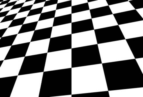
Figure 14-12 Checkerboard Procedural Texture
Example 14-19 Checker Fragment Shader with Conditional Checks
#version 300 es
precision mediump float;
// frequency of the checkerboard pattern
uniform int u_frequency;
in vec2 v_st;
layout(location = 0) out vec4 outColor;
void main()
{
vec2 tcmod = mod(v_st * float(u_frequency), 1.0);
if(tcmod.s < 0.5)
{
if(tcmod.t < 0.5)
outColor = vec4(1.0);
else
outColor = vec4(0.0);
}
else
{
if(tcmod.t < 0.5)
outColor = vec4(0.0);
else
outColor = vec4(1.0);
}
}
Example 14-20 Checker Fragment Shader without Conditional Checks
#version 300 es
precision mediump float;
// frequency of the checkerboard pattern
uniform int u_frequency;
in vec2 v_st;
layout(location = 0) out vec4 outColor;
void
main()
{
vec2 texcoord = mod(floor(v_st * float(u_frequency * 2)),2.0);
float delta = abs(texcoord.x − texcoord.y);
outColor = mix(vec4(1.0), vec4(0.0), delta);
}
As you can see, this was really easy to implement. We do see quite a bit of aliasing, which is never acceptable. With a texture checkerboard image, aliasing issues are overcome by using mipmapping and applying preferably a trilinear or bilinear filter. We now look at how to render an anti-aliased checkerboard pattern.
Anti-Aliasing of Procedural Textures
In Advanced RenderMan: Creating CGI for Motion Pictures, Anthony Apodaca and Larry Gritz give a very thorough explanation of how to implement analytic anti-aliasing of procedural textures. We use the techniques described in this book to implement our anti-aliased checker fragment shader. Example 14-21 describes the anti-aliased checker fragment shader code from the CheckerAA.rfx PVR_Shaman workspace in Chapter_14/PVR_ProceduralTextures.
Example 14-21 Anti-Aliased Checker Fragment Shader
#version 300 es
precision mediump float;
uniform int u_frequency;
in vec2 v_st;
layout(location = 0) out vec4 outColor;
void main()
{
vec4 color;
vec4 color0 = vec4(0.0);
vec4 color1 = vec4(1.0);
vec2 st_width;
vec2 fuzz;
vec2 check_pos;
float fuzz_max;
// calculate the filter width
st_width = fwidth(v_st);
fuzz = st_width * float(u_frequency) * 2.0;
fuzz_max = max(fuzz.s, fuzz.t);
// get the place in the pattern where we are sampling
check_pos = fract(v_st * float(u_frequency));
if (fuzz_max <= 0.5)
{
// if the filter width is small enough, compute
// the pattern color by performing a smooth interpolation
// between the computed color and the average color
vec2 p = smoothstep(vec2(0.5), fuzz + vec2(0.5),
check_pos) + (1.0 − smoothstep(vec2(0.0), fuzz,
check_pos));
color = mix(color0, color1,
p.x * p.y + (1.0 − p.x) * (1.0 − p.y));
color = mix(color, (color0 + color1)/2.0,
smoothstep(0.125, 0.5, fuzz_max));
}
else
{
// filter is too wide; just use the average color
color = (color0 + color1)/2.0;
}
outColor = color;
}
Figure 14-13 shows the checkerboard image rendered using the anti-aliased fragment shader in Example 14-18 with u_frequency = 10.

Figure 14-13 Anti-aliased Checkerboard Procedural Texture
To anti-alias the checkerboard procedural texture, we need to estimate the average value of the texture over an area covered by the pixel. Given a function g(v) that represents a procedural texture, we need to calculate the average value of (v) of the region covered by this pixel. To determine this region, we need to know the rate of change of g(v). The OpenGL ES Shading Language 3.00 contains derivative functions we can use to compute the rate of change of g(v) in x and y using the functions dFdx and dFdy. The rate of change, called the gradient vector, is given by [dFdx(g(v)), dFdy(g(v))]. The magnitude of the gradient vector is computed as sqrt ((dFdx(g(v))2 + dFdx(g(v))2). This value can also be approximated by abs(dFdx(g(v)))+abs(dFdy(g(v))). The function fwidth can be used to compute the magnitude of this gradient vector. This approach works well if g(v) is a scalar expression. If g(v) is a point, however, we need to compute the cross-product of dFdx(g(v)) and dFdy(g(v)). In the case of the checkerboard texture example, we need to compute the magnitude of thev_st.x and v_st.y scalar expressions and, therefore, the function fwidth can be used to compute the filter widths for v_st.x and v_st.y.
Let w be the filter width computed by fwidth. We need to know two additional things about the procedural texture:
• The smallest value of filter width k such that the procedural texture g(v) will not show any aliasing artifacts for filter widths less than k/2.
• The average value of the procedural texture g(v) over very large widths.
If w < k/2, we should not see any aliasing artifacts. If w > k/2 (i.e., the filter width is too large), aliasing will occur. We use the average value of g(v) in this case. For other values of w, we use a smoothstep to fade between the true function and average values. The full definition of the smoothstep built-in function is provided in Appendix B.
This discussion should have provided you with good insight into how to use procedural textures and how to resolve aliasing artifacts that become apparent when you are using procedural textures. The generation of procedural textures for many different applications is a very broad subject. The following list of references is a good place to start if you are interested in finding more information about procedural texture generation.
Further Reading on Procedural Textures
1. Anthony A. Apodaca and Larry Gritz. Advanced Renderman: Creating CGI for Motion Pictures (Morgan Kaufmann, 1999).
2. David S. Ebert, F. Kenton Musgrave, Darwyn Peachey, Ken Perlin, and Steven Worley. Texturing and Modeling: A Procedural Approach, 3rd ed. (Morgan Kaufmann, 2002).
3. K. Perlin. An image synthesizer. Computer Graphics (SIGGRAPH 1985 Proceedings, pp. 287–296, July 1985).
4. K. Perlin. Improving noise. Computer Graphics (SIGGRAPH 2002 Proceedings, pp. 681–682).
5. K. Perlin. Making noise. noisemachine.com/talkl/.
6. Pixar. The Renderman interface specification, version 3.2. July 2000. renderman.pixar.com/products/rispec/index.htm.
7. Randi J. Rost. OpenGL Shading Language, 2nd ed. (Addison-Wesley Professional, 2006).
Rendering Terrain with Vertex Texture Fetch
The next topic we cover is rendering terrain with the vertex texture fetch feature in OpenGL ES 3.0. In this example, we show how to render a terrain using a height map, as shown in Figure 14-14.
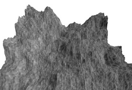
Figure 14-14 Terrain Rendered with Vertex Texture Fetch
Our terrain rendering example consists of two steps:
1. Generate a square grid for the terrain base.
2. Compute a vertex normal and fetch height values from the height map in the vertex shader.
Generating a Square Terrain Grid
The code in Example 14-22 generates a square triangle grid that we use as the base terrain.
Example 14-22 Terrain Rendering Flat Grid Generation
int ESUTIL_API esGenSquareGrid ( int size, GLfloat **vertices,
GLuint **indices )
{
int i, j;
int numIndices = (size−1) * (size−1) * 2 * 3;
// Allocate memory for buffers
if ( vertices != NULL )
{
int numVertices = size * size;
float stepSize = (float) size − 1;
*vertices = malloc ( sizeof(GLfloat) * 3 * numVertices );
for ( i = 0; i < size; ++i ) // row
{
for ( j = 0; j < size; ++j ) // column
{
(*vertices)[ 3 * (j + i*size) ] = i / stepSize;
(*vertices)[ 3 * (j + i*size) + 1 ] = j / stepSize;
(*vertices)[ 3 * (j + i*size) + 2 ] = 0.0f;
}
}
}
// Generate the indices
if ( indices != NULL )
{
*indices = malloc ( sizeof(GLuint) * numIndices );
for ( i = 0; i < size − 1; ++i )
{
for ( j = 0; j < size − 1; ++j )
{
// two triangles per quad
(*indices)[ 6*(j+i*(size−1)) ] = j+(i) *(size) ;
(*indices)[ 6*(j+i*(size−1))+1 ] = j+(i) *(size)+1 ;
(*indices)[ 6*(j+i*(size−1))+2 ] = j+(i+1)*(size)+1 ;
(*indices)[ 6*(j+i*(size−1))+3 ] = j+(i) *(size) ;
(*indices)[ 6*(j+i*(size−1))+4 ] = j+(i+1)*(size)+1 ;
(*indices)[ 6*(j+i*(size−1))+5 ] = j+(i+1)*(size) ;
}
}
}
return numIndices;
}
First, we generate the vertex position as a regularly spaced xy-coordinate in the [0, 1] range. The same xy-value can also be used as the vertex texture coordinate to look up the height value from the height map.
Second, we generate a list of indices for GL_TRIANGLES. A better method is to generate a list of indices for GL_TRIANGLE_STRIP, as you can improve the rendering performance by improving the vertex cache locality in the GPU.
Computing Vertex Normal and Fetching Height Value in Vertex Shader
Example 14-23 shows how to compute vertex normals and fetch height values from a height map in a vertex shader.
Example 14-23 Terrain Rendering Vertex Shader
#version 300 es
uniform mat4 u_mvpMatrix;
uniform vec3 u_lightDirection;
layout(location = 0) in vec4 a_position;
uniform sampler2D s_texture;
out vec4 v_color;
void main()
{
// compute vertex normal from height map
float hxl = textureOffset( s_texture,
a_position.xy, ivec2(−1, 0) ).w;
float hxr = textureOffset( s_texture,
a_position.xy, ivec2( 1, 0) ).w;
float hyl = textureOffset( s_texture,
a_position.xy, ivec2( 0, −1) ).w;
float hyr = textureOffset( s_texture,
a_position.xy, ivec2( 0, 1) ).w;
vec3 u = normalize( vec3(0.05, 0.0, hxr−hxl) );
vec3 v = normalize( vec3(0.0, 0.05, hyr−hyl) );
vec3 normal = cross( u, v );
// compute diffuse lighting
float diffuse = dot( normal, u_lightDirection );
v_color = vec4( vec3(diffuse), 1.0 );
// get vertex position from height map
float h = texture ( s_texture, a_position.xy ).w;
vec4 v_position = vec4 ( a_position.xy,
h/2.5,
a_position.w );
gl_Position = u_mvpMatrix * v_position;
}
The example provided in the Chapter_14/TerrainRendering folder shows a simple way of rendering terrain using a height map. If you are interested in finding out more about this topic, you can find many advanced techniques for efficiently rendering a large terrain model using the following list of references.
Further Reading on Large Terrain Rendering
1. Marc Duchaineau et al. ROAMing Terrain: Real-Time Optimally Adapting Meshes (IEEE Visualization, 1997).
2. Peter Lindstorm et al. Real-Time Continuous Level of Detail Rendering of Height Fields (Proceedings of SIGGRAPH, 1996).
3. Frank Losasso and Hugues Hoppe. Geometry Clipmaps: Terrain Rendering Using Nested Regular Grids, ACM Trans. Graphics (SIGGRAPH, 2004).
4. Krzystof Niski, Budirijanto Purnomo, and Jonathan Cohen. Multi-grained Level of Detail Using Hierarchical Seamless Texture Atlases (ACM SIGGRAPH I3D, 2007).
5. Filip Strugar. Continuous distance-dependent level of detail for rendering heightmaps ( Journal of Graphics, GPU and Game Tools, vol. 14, issue 4, 2009).
Shadows Using a Depth Texture
The next topic we cover is rendering shadows using a depth texture in OpenGL ES 3.0 using a two-rendering-pass algorithm:
1. In the first rendering pass, we draw the scene from the point of view of the light. We record the fragment depth value into a texture.
2. In the second rendering pass, we render the scene from the point of view of the eye position. In the fragment shader, we perform a depth test that determines whether the fragment is in the shadow by sampling the depth texture.
In addition, we use the percentage closer filtering (PCF) technique to sample the depth texture to generate soft shadows.
The result of executing the shadow rendering example from Chapter_14/Shadows is shown in Figure 14-15.
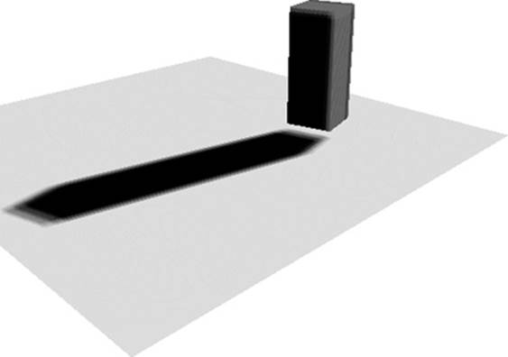
Figure 14-15 Shadow Rendering with a Depth Texture and 6 × 6 PCF
Rendering from the Light Position Into a Depth Texture
We render the scene from the point of view of the light into a depth texture using the following steps:
1. Set up a MVP matrix using the light position.
Example 14-24 shows the MVP transformation matrix generated by concatenating orthographic projection, model, and view transformation matrices.
Example 14-24 Set up a MVP Matrix from the Light Position
// Generate an orthographic projection matrix
esMatrixLoadIdentity ( &ortho );
esOrtho ( &ortho, −10, 10, −10, 10, −30, 30 );
// Generate a model matrix
esMatrixLoadIdentity ( &model );
esTranslate ( &model, −2.0f, −2.0f, 0.0f );
esScale ( &model, 10.0f, 10.0f, 10.0f );
esRotate ( &model, 90.0f, 1.0f, 0.0f, 0.0f );
// Generate a view−matrix transformation
// from the light position
esMatrixLookAt ( &view,
userData−>lightPosition[0],
userData−>lightPosition[1],
userData−>lightPosition[2],
0.0f, 0.0f, 0.0f,
0.0f, 1.0f, 0.0f );
esMatrixMultiply ( &modelview, &model, &view );
// Compute the final MVP
esMatrixMultiply ( &userData−>groundMvpLightMatrix,
&modelview, &ortho );
2. Create a depth texture and attach it to a framebuffer object.
Example 14-25 shows how to create a 1024 × 1024 16-bit depth texture to store the shadow map. The shadow map is set with a GL_LINEAR texture filter. When it is used with a sampler2Dshadow sampler type, we gain a hardware-based PCF, as the hardware will perform four depth comparisons in a single tap. We then show how to render into a framebuffer object with a depth texture attachment (recall that this topic was discussed in Chapter 12, “Framebuffer Objects”).
Example 14-25 Create a Depth Texture and Attach It to a Framebuffer Object
int InitShadowMap ( ESContext *esContext )
{
UserData userData = (UserData) esContext−>userData;
GLenum none = GL_NONE;
// use 1K x 1K texture for shadow map
userData−>shadowMapTextureWidth = 1024;
userData−>shadowMapTextureHeight = 1024;
glGenTextures ( 1, &userData−>shadowMapTextureId );
glBindTexture ( GL_TEXTURE_2D, userData−>shadowMapTextureId);
glTexParameteri ( GL_TEXTURE_2D, GL_TEXTURE_MAG_FILTER,
GL_NEAREST );
glTexParameteri ( GL_TEXTURE_2D, GL_TEXTURE_MIN_FILTER,
GL_LINEAR );
glTexParameteri ( GL_TEXTURE_2D, GL_TEXTURE_WRAP_S,
GL_CLAMP_TO_EDGE );
glTexParameteri ( GL_TEXTURE_2D, GL_TEXTURE_WRAP_T,
GL_CLAMP_TO_EDGE );
// set up hardware comparison
glTexParameteri( GL_TEXTURE_2D, GL_TEXTURE_COMPARE_MODE,
GL_COMPARE_REF_TO_TEXTURE );
glTexParameteri( GL_TEXTURE_2D, GL_TEXTURE_COMPARE_FUNC,
GL_LEQUAL );
glTexImage2D ( GL_TEXTURE_2D, 0, GL_DEPTH_COMPONENT16,
userData−>shadowMapTextureWidth,
userData−>shadowMapTextureHeight,
0, GL_DEPTH_COMPONENT, GL_UNSIGNED_SHORT,
NULL );
glBindTexture ( GL_TEXTURE_2D, 0 );
GLint defaultFramebuffer = 0;
glGetIntegerv ( GL_FRAMEBUFFER_BINDING,
&defaultFramebuffer );
// set up fbo
glGenFramebuffers ( 1, &userData−>shadowMapBufferId );
glBindFramebuffer ( GL_FRAMEBUFFER,
userData−>shadowMapBufferId );
glDrawBuffers ( 1, &none );
glFramebufferTexture2D ( GL_FRAMEBUFFER, GL_DEPTH_ATTACHMENT,
GL_TEXTURE_2D,
userData−>shadowMapTextureId, 0 );
glActiveTexture ( GL_TEXTURE0 );
glBindTexture ( GL_TEXTURE_2D, userData−>shadowMapTextureId);
if ( GL_FRAMEBUFFER_COMPLETE !=
glCheckFramebufferStatus ( GL_FRAMEBUFFER ) )
{
return FALSE;
}
glBindFramebuffer ( GL_FRAMEBUFFER, defaultFramebuffer );
return TRUE;
}
3. Render the scene using a pass-through vertex and fragment shader.
Example 14-26 provides the vertex and fragment shaders used to render the scene to the depth texture from the point of view of the light. Both shaders are very simple, as we need simply to record the fragment depth value into the shadow map texture.
Example 14-26 Rendering to Depth Texture Shaders
// vertex shader
#version 300 es
uniform mat4 u_mvpLightMatrix;
layout(location = 0) in vec4 a_position;
out vec4 v_color;
void main()
{
gl_Position = u_mvpLightMatrix * a_position;
}
// fragment shader
#version 300 es
precision lowp float;
void main()
{
}
To use these shaders, in the host code prior to rendering the scene, we clear the depth buffer and disable color rendering. To avoid the creation of a shadow rendering artifact due to a precision problem, we can use a polygon offset command to increase the depth values written to the texture.
// clear depth buffer
glClear( GL_DEPTH_BUFFER_BIT );
// disable color rendering; only write to depth buffer
glColorMask ( GL_FALSE, GL_FALSE, GL_FALSE, GL_FALSE );
// reduce shadow rendering artifact
glEnable ( GL_POLYGON_OFFSET_FILL );
glPolygonOffset( 4.0f, 100.0f );
Rendering from the Eye Position with the Depth Texture
We render the scene from the point of view of the light into a depth texture using the following steps:
1. Set up a MVP matrix using the eye position.
The MVP matrix setup consists of the same code as in Example 14-24, with the exception that we create the view transformation matrix by passing the eye position to the esMatrixLookAt call as follows:
// create a view−matrix transformation
esMatrixLookAt ( &view,
userData−>eyePosition[0],
userData−>eyePosition[1],
userData−>eyePosition[2],
0.0f, 0.0f, 0.0f,
0.0f, 1.0f, 0.0f );
2. Render the scene using the shadow map created in the first rendering pass.
Example 14-27 shows the vertex and fragment shaders that we use to render the scene from the eye position.
Example 14-27 Rendering from the Eye Position Shaders
// vertex shader
#version 300 es
uniform mat4 u_mvpMatrix;
uniform mat4 u_mvpLightMatrix;
layout(location = 0) in vec4 a_position;
layout(location = 1) in vec4 a_color;
out vec4 v_color;
out vec4 v_shadowCoord;
void main()
{
v_color = a_color;
gl_Position = u_mvpMatrix * a_position;
v_shadowCoord = u_mvpLightMatrix * a_position;
// transform from [−1,1] to [0,1];
v_shadowCoord = v_shadowCoord * 0.5 + 0.5;
}
// fragment shader
#version 300 es
precision lowp float;
uniform lowp sampler2DShadow s_shadowMap;
in vec4 v_color;
in vec4 v_shadowCoord;
layout(location = 0) out vec4 outColor;
float lookup ( float x, float y )
{
float pixelSize = 0.002; // 1/500
vec4 offset = vec4 ( x * pixelSize * v_shadowCoord.w,
y * pixelSize * v_shadowCoord.w,
0.0, 0.0 );
return textureProj ( s_shadowMap, v_shadowCoord + offset );
}
void main()
{
// 3x3 kernel with 4 taps per sample, effectively 6x6 PCF
float sum = 0.0;
float x, y;
for ( x = −2.0; x <= 2.0; x += 2.0 )
for ( y = −2.0; y <= 2.0; y += 2.0 )
sum += lookup ( x, y );
// divide sum by 9.0
sum = sum * 0.11;
outColor = v_color * sum;
}
In the vertex shader, we transform the vertex position twice: (1) using the MVP matrix created from the eye position and (2) using the MVP matrix created from the light position. The former result is recorded into gl_Position, while the latter result is recorded into v_shadowCoord. Note that the v_shadowCoord result is exactly the same vertex position result when we render to the shadow map. Armed with this knowledge, we can use the v_shadowCoord as the texture coordinate to sample into the shadow map by first transforming the coordinate from homogeneous coordinate [–1, 1] space into [0, 1] space in the vertex shader. Alternatively, we can avoid performing these calculations in the vertex shader by pre-multiplying the MVP matrix from the light position with the following bias matrix in the host code:
0.5, 0.0, 0.0, 0.0,
0.0, 0.5, 0.0, 0.0,
0.0, 0.0, 0.5, 0.0,
0.5, 0.5, 0.5, 1.0
In the fragment shader, we check the current fragment to determine whether it is in the shadow by sampling the shadow map using the v_shadowCoord and textureProj call. We perform 3 × 3 kernel filtering to further increase the effect of PCF (effectively 6 × 6 PCF when combined with four hardware depth comparisons per tap). Then we average the shadow map sample result to modulate the fragment color. When the fragment is in shadow, the sample result will be zero and the fragment will be rendered in black.
Summary
This chapter explored how many of the OpenGL ES 3.0 features presented throughout this book can be applied to achieve various rendering techniques. This chapter covered rendering techniques that made use of features including cubemaps, normal maps, point sprites, transform feedback, image postprocessing, projective texturing, framebuffer objects, vertex texture fetch, shadow maps, and many shading techniques. Next, we will return to the API to discuss the functions your application can use to query OpenGL ES 3.0 for information.
All materials on the site are licensed Creative Commons Attribution-Sharealike 3.0 Unported CC BY-SA 3.0 & GNU Free Documentation License (GFDL)
If you are the copyright holder of any material contained on our site and intend to remove it, please contact our site administrator for approval.
© 2016-2026 All site design rights belong to S.Y.A.