The Essential Guide to SAS Dates and Times, Second Edition (2014)

Chapter 6. Deeper into Dates and Times with SAS

6.1 Macro Variables and Dates

There is a high potential for confusion when it comes to the subject of macro variables and dates. Although you have access to dates and times in the SAS macro language with the automatic macro variables &SYSDATE, &SYSDATE9, &SYSDAY, and &SYSTIME, the display of these values is fixed, and therefore they do not give you the power of SAS formats, or of SAS date and time functions.

6.1.1 Automatic Macro Variables

None of these automatic macro variables can be assigned values with %LET or CALL SYMPUT(), or by any other means. They are read-only and work by reading the operating system clock when a SAS session is started. This means that they do not change within a given SAS session.

&SYSDATE

&SYSDATE cannot be modified and displays the system date as a SAS date value formatted with the DATE7. format. If the date according to the operating system when the SAS session starts is July 17, 2014, then &SYSDATE would be equal to "17JUL14."

&SYSDATE9

&SYSDATE9 is identical to &SYSDATE, except that it formats the system date with the DATE9. format and is therefore Y2K-compliant. If the operating system date is November 22, 2015, then &SYSDATE9 would be equal to "22NOV2015."

&SYSDAY

&SYSDAY displays the name of the day that the SAS session began (according to the operating system). If you started a SAS job or session on Monday, April 14, 2014, &SYSDAY would be equal to "Monday."

&SYSTIME

&SYSTIME displays the system time (according to the operating system) in TIME5. format. If the system time is 3:36 p.m. when you start SAS, then &SYSTIME would be equal to "15:36."

6.1.2 Putting Dates into Titles

One of the prime uses of dates in macro variables is for custom titles and footnotes. To use a macro variable in a title, you just need to enclose the TITLE or FOOTNOTE statement that contains the macro variable with double quotation marks like this:

TITLE "Today's Date is &SYSDATE9";

To see this in context, look at the following program:

Example 6.1: Using Automatic Macro Variables in a Title

TITLE "This is how to put a macro variable in a title: Today's Date is &SYSDATE9";

ODS RTF FILE="examples\title.rtf";

PROC PRINT DATA=sashelp.company (OBS=5);

ID job1;

VAR depthead;

RUN;

ODS RTF CLOSE;

Here is the resulting output:

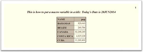
While the automatic macro variables &SYSDATE, &SYSDATE9, &SYSDAY, and &SYSTIME might give you the information that you need, their formats are fixed and cannot be changed. Given the multiple ways that dates, times, and datetimes can be displayed, it would be good if you could use the formats and functions to get the display of dates and times that you want in your titles.

6.1.3 Using %SYSFUNC() to Create Dates, Times, and Datetimes in Macro Variables

Many of the date and time functions, as well as formats, are available in the SAS macro language through the %QSYSFUNC() and %SYSFUNC() macro functions. When you are using one of these macro functions with dates and times, you can use two arguments: The first is the date, time, or datetime function that you wish to use. The second argument is optional, but you can specify the format that should be applied to the result.

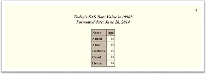
Example 6.2: Date Functions with %SYSFUNC()

This example puts the formatted value of today's date into the macro variable &DATE and demonstrates the difference between unformatted and formatted dates in macro variables. The date value in &RAWDATE is stored in macro space as a text string and will need to be converted if you want to use it for any calculations. &DATE is also a text string in macro space, but it shows that the WORDDATE. format has been applied to the value.

%LET rawdate=%SYSFUNC(DATE());

%LET date=%SYSFUNC(DATE(),WORDDATE32.);

TITLE "Today's SAS Date Value is &rawdate";

TITLE2 "Formatted date: &date";

ODS RTF FILE="c:\book\2ndEd\examples\title2.rtf";

PROC PRINT DATA=sashelp.class (OBS=5);

ID name;

VAR age;

RUN;

ODS RTF CLOSE;

Now you can use the result in a title or footnote.

You can also use this as a part of an output file name or Excel worksheet name.

Example 6.3: Putting a Date Value into an Output File Name

%LET filedate=%SYSFUNC(DATE(),yymmddd10.);

ODS RTF FILE="Car_Report_&filedate..rtf";

PROC PRINT DATA=sashelp.cars NOOBS LABEL;

RUN;

ODS RTF CLOSE;

When you try this at home, you will see that you have generated an RTF file named "Car_report_yyyy-mm-dd.rtf."

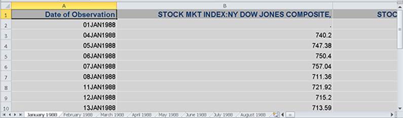
Example 6.4: Naming Worksheets with the Date

In this example, we create a custom format to display dates as the full month name and 4-digit year and apply it to a copy of the date variable in the data set. Then we use that variable as the BY variable in the PRINT procedure. Not only does this put the name on each worksheet, but it also filters the dates into their correct worksheet without much extra coding required. There are many other ways that you can accomplish this task, but this is straightforward and simple. If you have a great deal of data, you might want to investigate a more efficient method than creating an additional variable in a data set. Lines 1–5 create the format using the PICTURE statement in PROC FORMAT and date directives discussed in section 2.6, and lines 6–13 create our duplicate variable with our custom format and also subset the data set. Note the date literals used as values in the BETWEEN operator in line 10. We remove the default BY line from the output in line 14. The SHEET_NAME option allows us to use the BY value token (#BYVAL1) as the name of the worksheet.

1 PROC FORMAT;

2 PICTURE namefmt

3 LOW-HIGH='%B %Y' (DATATYPE=date)

4 ;

5 RUN;

6 PROC SQL;

7 CREATE TABLE subset AS

8 SELECT date as sheet_date FORMAT=namefmt15., *

9 FROM sashelp.citiday

10 WHERE date BETWEEN '01JAN1988'd AND '31AUG1988'd

11 ORDER BY DATE

12 ;;;;

13 QUIT;

14 OPTIONS NOBYLINE;

15 ODS TAGSETS.EXCELXP FILE="ex6.1.4.xml" OPTIONS (SHEET_NAME="#BYVAL1");

16 PROC PRINT DATA=subset LABEL NOOBS;

17 BY sheet_date;

18 RUN;

19 ODS TAGSETS.EXCELXP CLOSE;

This is the resulting workbook:

6.1.4 Using Dates in Macros

While SAS can handle dates, times, and datetime values as numbers, getting the macro processor to accept them as numbers might involve an extra step or two. Let's look at the following code:

1 %MACRO date_loop;

2 %DO I='05JUN2014'd %TO '12JUN2014'd;

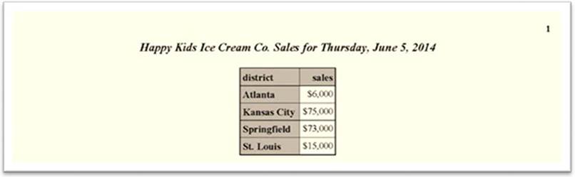
3 TITLE "Happy Kids Ice Cream Co. Sales for &i";

4 PROC PRINT DATA =sample.dailysales;

5 ID district;

6 VAR sales;

7 WHERE date EQ &i;

8 RUN;

9 %END;

10 %MEND;

We have used two date literals to provide the period over which we want the report run and used it in the title as well. What happens when this is submitted?

ERROR: A character operand was found in the %EVAL function or %IF condition where a numeric operand is required. The condition was: '05JUN2014'd

ERROR: The %FROM value of the %DO I loop is invalid.

ERROR: A character operand was found in the %EVAL function or %IF condition where a numeric operand is required. The condition was: '12JUN2014'd

ERROR: The %TO value of the %DO I loop is invalid.

ERROR: The macro DATE_LOOP will stop executing.

To the macro processor, the date literals are only text. They do not function as they do in the rest of SAS. How can we get around this? By using the %SYSEVALF() macro function to force the interpretation of the date literals. Let's replace line 2 with the following line:

%DO i=%SYSEVALF('05JUN2014'd) %TO %SYSEVALF('12JUN2014'd);

Now the loop will execute properly. However, the date in the title does not look good at all.

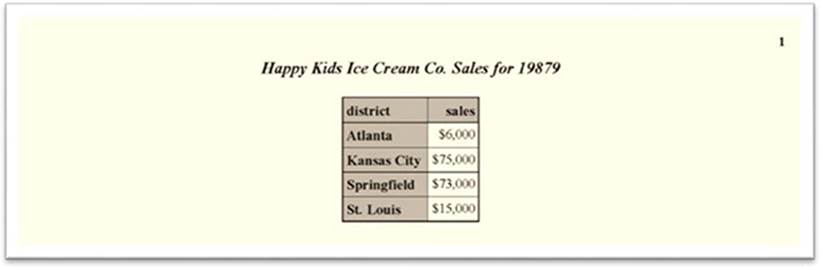
The date in the title doesn't look like a date. We need to make one more modification to the program to get our title to look right. The %LET statement added in line 3 creates a formatted value of the date in the macro loop for use. The PUTN() function is used here instead of the PUT() function because you can't use the PUT() function with %SYSFUNC() or QSYSFUNC().

1 %MACRO date_loop;

2 %DO I=%SYSEVALF('05JUN2014'd) %TO %SYSEVALF('12JUN2014'd);

3 %LET TITLEDATE=%SYSFUNC(PUTN(&i,WORDDATE.));

4 TITLE "Happy Kids Ice Cream Co. Sales for &titledate";

5 PROC PRINT DATA=sample.dailysales;

6 ID district;

7 VAR sales;

8 WHERE date EQ &i;

9 RUN;

10 %END;

11 %MEND;

And now we get the desired result.

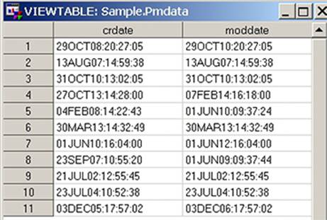
Our final example of using dates in macros demonstrates how to get a date from a data set into a macro. For this example, we want to put the latest date from a given column into a macro variable so that it can be used in a title. Let's look at some timing variables from this sample data set. We want to put the latest date and time (which is in record 4) from the variable MODDATE (nicely formatted, of course) on the title of each page.

Method 1: Using CALL SYMPUT

The CALL SYMPUT() and SYMGET() functions are also used to communicate between the DATA step and the macro world. CALL SYMPUT()takes a value and stores it in macro space from within a DATA step, while SYMGET() takes a macro variable and enables you to use it in a DATA step. In this situation, I recommend that you use CALL SYMPUTX() instead of CALL SYMPUT(), because CALL SYMPUTX() suppresses any trailing blanks in the macro variable created, and the presence of trailing blanks might affect the justification of your title or footnote. The difference between run-time and compile time is very important. You cannot use a %LET statement to store macro values that are defined during execution of a DATA step. You also cannot use a macro variable reference (with an ampersand [&]) in the same DATA step where the macro variable is created with CALL SYMPUT(). The next example uses what was discussed in section 6.1.2 to show how you can obtain a date value from a SAS data set and then put it in a macro variable to use in a title. Since the DATETIME. format isn't formal enough for this report, we're going to create a RPTDATE. custom format.

PROC FORMAT;

PICTURE rptdate (DEFAULT=32)

. - .Z = 'Missing'

LOW-HIGH = '%B %d, %Y at %I:%0M %p' (DATATYPE=DATETIME);

RUN;

/* Get the maximum date in the variable */

PROC MEANS DATA=sample.pmdata MAX NOPRINT;

VAR moddate;

OUTPUT OUT=tmp MAX=max;

RUN;

/*Transfer it to a macro variable using CALL SYMPUTX() */

DATA _NULL_;

SET tmp;

CALL SYMPUTX('lastmod',STRIP(PUT(max,rptdate.)));

RUN;

%PUT lastmod=&lastmod;

Partial Log

42 %PUT lastmod=&lastmod;

lastmod=February 7, 2014 at 4:18 PM

Method 2: Using PROC SQL

For something as simple as the highest (or lowest) value in a date or datetime variable, you don't have to use a SAS procedure and a DATA step. PROC SQL can take the place of both.

PROC SQL NOPRINT;

SELECT DISTINCT STRIP(PUT(MAX(moddate),rptdate.)) LENGTH=32 INTO :lastmod

FROM sample.pmdata;

QUIT;

%PUT lastmod=&lastmod;

The Log

1 PROC SQL NOPRINT;

2 SELECT DISTINCT STRIP(PUT(MAX(moddate),rptdate.)) LENGTH=32 INTO

3 ! :lastmod

4 FROM sample.pmdata;

5 QUIT;

NOTE: PROCEDURE SQL used (Total process time):

real time 0.08 seconds

cpu time 0.00 seconds

6

7 %PUT lastmod=&lastmod;

lastmod=February 7, 2014 at 4:18 PM

Whichever method you choose, the macro variable &LASTMOD, containing the value "February 7, 2014 at 4:18 PM", is ready to use in your report title.

6.2 Graphing Dates

When you use dates, times, or datetime values in your SAS graphics, you have to remember that they are numbers. This has a large impact on the axes and labeling of your graphics. Attempting to graph a result over a period of time without using formats or intervals will usually result in a graph that is not clear or well-defined. The good news is that you can use all the features associated with SAS dates to improve your graphics, such as formats and intervals. The following series of examples will illustrate. Example 6.5 will demonstrate the graphing of dates with SAS/GRAPH, while Example 6.6 will use ODS graphics to produce a series plot.

Johnny's Savings Account

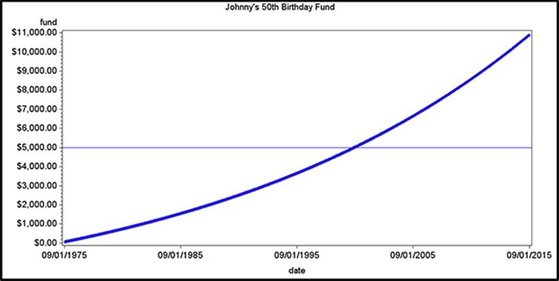
When Johnny turned 10 years old on September 1, 1975, he took all the money that he had in his piggy bank and deposited it into a bank account that paid 3.5% interest annually, compounded daily. He promised himself that he would add two dollars at the end of each week and that he would take the money out when he reached the ripe old age of 50. When he was 10, Johnny thought he might have $4,000 by the time he reached age 50. He kept that promise, so let's look at Johnny's earnings from the time he was 10 until he was 50 using the following program:

Example 6.5: SAS/GRAPH

TITLE "Johnny's 50th Birthday Fund";

PROC GPLOT DATA=book.graph1;

PLOT fund*date / VREF=5000 LV=1 CV=blue;

RUN;

Here is the resulting graph:

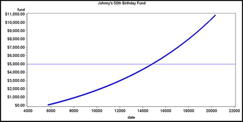
Unfortunately, the result of this simple example isn't helpful. We can see that Johnny started around 6000, and he turned 50 somewhere around 20000. What does that mean? This should be easy enough to fix. Don't we just need to add a FORMAT statement?

TITLE "Johnny's 50th Birthday Fund";

PROC GPLOT DATA=book.graph1;

PLOT fund*date / VREF=5000 LV=1 CV=blue;

FORMAT date mmddyy10.; /* Add FORMAT statement */

RUN;

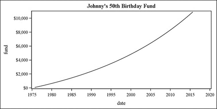
Here is the new GPLOT graph with the FORMAT statement:

What has happened here is that SAS chose the boundaries and figured out major and minor tick marks. In this example, it has selected major intervals at decade boundaries, and minor ones at year boundaries. That's not a bad choice for this example, but SAS/GRAPH doesn't always make such a good choice when selecting the boundaries of an axis. Can't you define the horizontal axis yourself? Of course, you can! Johnny was born in September, so it would make sense to chart his progress at his birthdays and restrict the span of the horizontal axis to the period during which he's contributing.

TITLE "Johnny's 50th Birthday Fund";

PROC GPLOT DATA=book.graph1;

PLOT fund*date / VREF=5000 LV=1 CV=blue

HAXIS='01SEP1975'd TO '01SEP2015'd by YEAR;

FORMAT date mmddyy10.;

RUN;

Here is the new graph that we get from using the HAXIS option in the PLOT statement to specify the axis range:

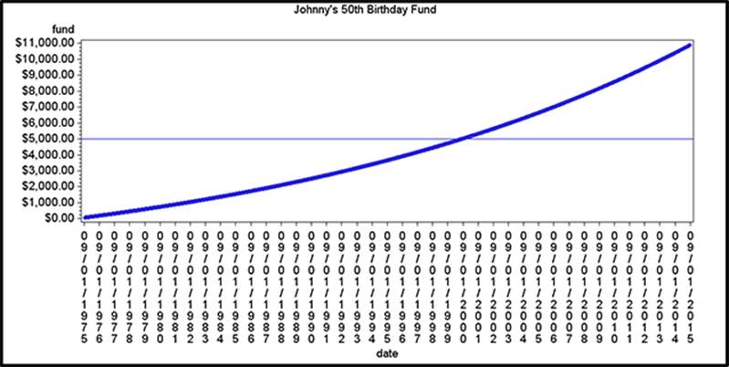
What happened? We defined the horizontal axis as having tick marks every year, so SAS accommodated our request. Since there was not enough room to display the values horizontally, SAS automatically rotated the values 90 degrees. Unfortunately, that left less space for the graph itself. We need better spacing on our horizontal axis.

Since decades seemed to work well, let's use those as our intervals, but we want to start on Johnny's 10th birthday, and define the major horizontal axis points at September 1, 1975, September 1, 1985, September 1, 1995, September 1, 2005, and September 1, 2015. An interval multiplier of 10 will create the decade interval, and a shift operator of 69 (60 [months in 5 years] plus 9 [months from January to September]) will move the starting date of the 10-year interval to September 1975 so that it matches the starting point of the horizontal axis. Note that the only change from the previous version is in the interval definition.

TITLE "Johnny's 50th Birthday Fund";

PROC GPLOT DATA=book.graph1;

PLOT fund*date / VREF=5000 LV=1 CV=blue

HAXIS='01SEP1975'd TO '01SEP2015'd by YEAR10.69;

FORMAT date mmddyy10.;

RUN;

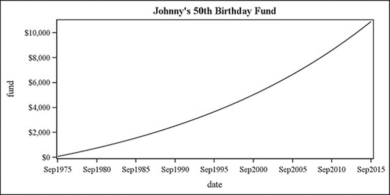
Here is the final product:

Now that's what we wanted. This demonstrates that you have all of the interval types, as well as their multipliers and shift operators, available when you are defining axes that involve date, time, and datetime values in SAS/GRAPH. It makes defining the exact scope of the graph much easier, not to mention comprehending what you've graphed.

Example 6.6: ODS Graphics

We will continue to use Johnny's 50th birthday fund for the SGPLOT series of examples. The SGPLOT procedure has a way of assigning a time scale to an axis by setting the axis TYPE option in the XAXIS statement equal to TIME, and the SERIES style of plot is perfect for graphs of longitudinal data.

Here's the basic SGPLOT from the above code.

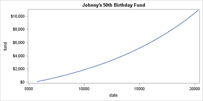
As with the GPLOT example, an unformatted date variable isn't very useful. However, even though we got our graph, SGPLOT did not run smoothly. In order to produce this graph, the procedure made some adjustments in order to produce the graph. Let's look at the log from the program that produced the above graph.

3 TITLE "Johnny's 50th Birthday Fund";

4 PROC SGPLOT DATA=book.graph1;

5 XAXIS TYPE=time;

6 SERIES X=date Y=fund;

7 RUN;

NOTE: PROCEDURE SGPLOT used (Total process time):

real time 1.20 seconds

cpu time 0.09 seconds

NOTE: Time axis can only support date time values. The axis type will be changed to LINEAR. ❶

NOTE: There were 2435 observations read from the data set

BOOK.GRAPH1.

Note ❶ is telling us that you can't use the TYPE value of TIME. But aren't we graphing dates? The SGPLOT procedure relies on formats to determine that the data being graphed are dates or times. Without it, SGPLOT errs on the side of caution and just assumes that you are graphing linear data. This will create a plot for data graphed along a sequence (such as dates), so it looks right, but it is not clear that you are graphing dates.

Let's add the missing format to our SGPLOT:

TITLE "Johnny's 50th Birthday Fund";

PROC SGPLOT DATA=book.graph1;

XAXIS TYPE=time;

SERIES X=date Y=fund;

FORMAT date monyy7.;

RUN;

That looks better, even though SAS did not use the MONYY7. format that you requested and substituted one of its own as seen in note ❶ below.

51 TITLE "Johnny's 50th Birthday Fund";

52 PROC SGPLOT DATA=book.graph1;

53 XAXIS TYPE=time;

54 SERIES X=date Y=fund;

55 FORMAT date monyy7.;

56 RUN;

NOTE: PROCEDURE SGPLOT used (Total process time):

real time 0.90 seconds

cpu time 0.20 seconds

❶ NOTE: The column format MONYY7 is replaced by an auto-generated format

on the axis.

This is really the same problem as with SAS/GRAPH when you haven't defined the tick marks on the X axis properly. The VALUES= option in the XAXIS statement allows us to define our scale in the same way that the HAXIS= option in the PLOT statement does in SAS/GRAPH. For a 50-year period, let's try 5-year intervals, starting when Johnny made his promise on September 1, 1975.

TITLE "Johnny's 50th Birthday Fund";

PROC SGPLOT DATA=book.graph1;

XAXIS TYPE=time VALUES=('01sep1975'd TO '01sep2015'd BY YEAR5);

SERIES X=date Y=fund;

FORMAT date monyy7.;

RUN;

Now the display looks much nicer, and we have our MONYY7. format displayed.

6.3 The Basics of PROC EXPAND

The EXPAND procedure is a part of SAS/ETS, which is used to prepare time series data for further analysis. It creates a SAS data set and does not produce printed output.

6.3.1 Capabilities of PROC EXPAND

PROC EXPAND will change the sampling frequency of the data that you have and convert it to a different one. It can interpolate values in time series data, for example, when you have quarterly data that you need to report or analyze on a monthly basis. It can perform the reverse operation, that is, to aggregate (collapse) data from a higher sampling frequency to a lower one, such as taking monthly data and turning it into quarterly data. PROC EXPAND can interpolate missing values even if you aren't changing the sampling frequency. It also provides for extensive data transformations and performs all of these functions without a lot of DATA step programming. The SAS/ETS documentation provides detail on the procedure, its statements, and the options for those statements. There are other procedures available in SAS/ETS, such as TIMESERIES and TIMEDATA, that can be used to manipulate time series data, and if you need to work with time series data on a regular basis, you should investigate the SAS/ETS product and its documentation more carefully.

PROC EXPAND uses SAS interval definitions. This includes interval multipliers and the shift index. For a detailed explanation of intervals, interval multipliers, and the interval shift index, see Sections 5.5 and 5.6 of this book. When you use these interval definitions (plus any shift index and/or multipliers), PROC EXPAND will automatically adjust for any calendar effects (leap years, varying number of days in a month). As with anything that uses these interval definitions, all measurements and calculations are considered to be at the beginning of the interval(s) specified. It is possible to change that definition with options in one of the PROC EXPAND statements, and those are discussed in Section 6.3.5.

PROC EXPAND Sample Data

The following data set will be used for the examples in this section. This is monthly total light rail ridership data obtained from the American Public Transportation Association for the years 2003 and 2004 and is used with their permission. The values for October and November 2003 were removed from the data to demonstrate some of the capabilities of PROC EXPAND.

6.3.2 Using PROC EXPAND to Convert to a Higher Frequency

You can use PROC EXPAND to convert data from a lower sampling frequency to a higher sampling frequency (for example, converting monthly data to daily or weekly data). It does so by interpolation, and the syntax to convert to a higher sampling frequency is as follows:

Example 6.7: Converting to a Higher Sampling Frequency

1 PROC EXPAND DATA=book.month OUT=seven_days FROM=MONTH TO=WEEK;

2 ID date;

3 CONVERT riders;

4 RUN;

The PROC EXPAND statement in line 1 specifies the output data set (SEVEN_DAYS) and explains how the data in BOOK.MONTH should be converted, from MONTH intervals to WEEK intervals. The ID statement in line 2 indicates the variable that identifies the time of each record. Since the WEEK interval begins on Sunday, the dates will be aligned on Sundays. If you want the dates to align to a different day of the week, use a shift indicator. The WEEK.2 interval will align the dates to Mondays; the WEEK.3 interval aligns to Tuesdays, and so on.

You will usually use an ID statement with PROC EXPAND. Otherwise, SAS will create an ID variable for the input records and use the starting point of January 1, 1960, which might not be what you want. The CONVERT statement identifies the variable(s) to convert. You can also rename the variable(s) being converted in the output data set like this: CONVERT input-var=output-var; Here are the first eight observations from the data set SEVEN_DAYS produced by the above code:

When you interpolate time series data to a higher frequency, consider that the interpolated values do not add any new information to the data because they have been derived mathematically, not observed. Therefore, any statistical analyses performed with these interpolated data should be viewed with caution.

6.3.3 Using PROC EXPAND to Convert to a Lower Frequency

You can convert data to a lower frequency with PROC EXPAND in two ways: First, you can use the same syntax as with converting to a higher sampling frequency, except that the TO= interval would be of a lower sampling frequency. When you convert your data this way, PROC EXPAND performs interpolation for missing values using a curve-fitting method, which allows for conversion between intervals that aren't nested. A nested interval is one that fits wholly inside another interval (for example, days nest within weeks, because there are exactly seven days in a week, but weeks do not nest within months, because most months have partial weeks). The following program will interpolate any missing values in our data by fitting a cubic spline function through the existing data before converting the data from a month frequency to a quarter frequency.

Example 6.8: Converting to a Lower Frequency

PROC EXPAND DATA=book.month OUT=quarterly FROM=MONTH TO=QTR;

ID date;

CONVERT riders;

RUN;

The resulting data set QUARTERLY (above) has eight observations, four for each year, synchronized on the QTR interval boundaries. As you can see, the data that were missing from our original data set (for October 2003) are interpolated.

The second method enables you to perform simple aggregation (addition) without interpolation of missing values. The AGGREGATE method always produces an exact result without interpolation, and it requires that the intervals be nested. This program shows the result of a simple aggregation on our sample data:

Example 6.9: Performing Aggregation without Interpolation

PROC EXPAND DATA=book.month OUT=annual FROM=MONTH TO=YEAR;

ID date;

CONVERT riders / METHOD=AGGREGATE;

RUN;

Example 6.10: The Importance of the ID Statement in PROC EXPAND

The following PROC EXPAND step has no ID statement. Let's run it so that we can see the assumptions that SAS makes in its absence. This illustrates why the ID statement is almost always used with this procedure:

PROC EXPAND DATA=book.month OUT=ANNUAL FROM=MONTH TO=YEAR;

CONVERT riders;

RUN;

How did we wind up with data for 1960 and 1961 when we used data from 2003 and 2004? If there is no ID variable to indicate the dates, SAS will create ID values to label the input records, and it will start from its zero point, January 1, 1960.

6.3.4 Using PROC EXPAND to Interpolate Missing Values

PROC EXPAND can also be used to interpolate missing values without converting frequencies. There are two ways to do this; use the one that fits your situation. If you are interpolating missing values at specific points in time, leave off the FROM= and TO= options, but make sure that you use an ID statement to indicate the variable that contains the time points of the observed values. The time points do not have to be evenly spaced, nor do you need a record for each time point within the interval. PROC EXPAND will read the values supplied in the ID variable and will fit a spline function through the available data points. It then fills in the missing values based on that fitted spline. Remember that the data for the months of October and November are missing in our sample table. The following program demonstrates:

Example 6.11: Interpolating Missing Values

PROC EXPAND DATA=book.month OUT=nomiss;

ID date;

CONVERT riders;

RUN;

The bolded and italicized values in the following table are the result of the interpolation performed by PROC EXPAND.

The second method interpolates missing values in a time series without converting the observation frequency. Use this when you want to fill in the missing values and maintain the same observation frequency. It requires the FROM= option, but leave off the TO= option, as shown here:

PROC EXPAND DATA=book.month OUT=nomiss2 FROM=MONTH;

ID date;

CONVERT riders;

RUN;

By default, the interpolation is performed by fitting the points to a cubic spline curve. You can request other methods of interpolation with the METHOD= option in the CONVERT statement, and these are detailed in the SAS/ETS documentation. PROC EXPAND will ignore observations that have missing values for the ID variable, even if there are data points for the CONVERT variable(s). Table 6.1 is a summary of what PROC EXPAND does when there are missing values for the ID variable and/or CONVERT data points.

Table 6.1: How PROC EXPAND Handles Interpolation of Missing Values in Input Data

6.3.5 The OBSERVED= Option for the CONVERT Statement in PROC EXPAND

As with the other uses of SAS date, time, and datetime intervals, the default for PROC EXPAND is to consider the values as being from the beginning of the intervals provided in the FROM= and TO= options. This is not always the case with real-world data, and it can cause very different results, especially if the values are not measured at the beginning of the given interval(s), or they do not represent a single observed value for a specific point in time. You can control how the SAS intervals are used with the OBSERVED option in the CONVERT statement. There are six possible values for the OBSERVED= option, as shown in Table 6.2:

Table 6.2: Values for the OBSERVED= Option

The syntax of the OBSERVED= option is:

1. OBSERVED=value OR

2. OBSERVED=(from-value, to-value)

value is one of the keywords in table 6.2, from indicates the characteristics of the data from which you are converting, and to represents the characteristics of the data resulting from the conversion. Using form 1 is the same as specifying the same value for both from and to; that is, OBSERVED=AVERAGE is the same as OBSERVED=(AVERAGE,AVERAGE). Again, if you do not supply an OBSERVED option for the conversion, it is the same as using OBSERVED=(BEGINNING,BEGINNING).

Examples 6.12 and 6.13 demonstrate how different combinations of the OBSERVED= option affect our sample data when we increase and decrease the sampling frequency. The program below shows the code to increase the sampling frequency. It also shows how to rename the output variables in the CONVERT statement by placing an equal sign (=) after the data set variable and providing the new variable name afterward.

Example 6.12: Effect of Different Values for OBSERVED= Option on Increased Frequency

/* The effect of the different values for the OBSERVED option of

the CONVERT statement in PROC EXPAND on increased sample frequency */

PROC EXPAND DATA=book.month OUT=seven1 FROM=MONTH TO=WEEK;

ID date;

CONVERT riders=beginning / OBSERVED=BEGINNING /*Default */;

RUN;

PROC EXPAND DATA=book.month OUT=seven2 FROM=MONTH TO=WEEK;

ID date;

CONVERT riders=middle / OBSERVED=MIDDLE;

RUN;

PROC EXPAND DATA=book.month OUT=seven3 FROM=MONTH TO=WEEK;

ID date;

CONVERT riders=end / OBSERVED=END;

RUN;

PROC EXPAND DATA=book.month OUT=seven4 FROM=MONTH TO=WEEK;

ID date;

CONVERT riders=total / OBSERVED=TOTAL;

RUN;

PROC EXPAND DATA=book.month OUT=seven5 FROM=MONTH TO=WEEK;

ID date;

CONVERT riders=average / OBSERVED=AVERAGE;

RUN;

PROC EXPAND DATA=book.month OUT=seven6 FROM=MONTH TO=WEEK;

ID date;

CONVERT riders=begend / OBSERVED=(BEGINNING,END);

RUN;

PROC EXPAND DATA=book.month OUT=seven7 FROM=MONTH TO=WEEK;

ID date;

CONVERT riders=avetot / OBSERVED=(AVERAGE,TOTAL);

RUN;

DATA compare_lo;

MERGE seven1 seven2 seven3 seven4 seven5 seven6 seven7;

BY date;

LABEL

beginning="BEGINNING" middle = "MIDDLE" end = "END" average = "AVERAGE"

total = "TOTAL" begend = "BEGINNING,END" avetot = "AVERAGE,TOTAL"

;;;

FORMAT beginning--avetot 7.2;

RUN;

PROC REPORT DATA=compare_lo NOWD SPLIT='\';

COLUMNS date ('OBSERVED=\Option Value' beginning middle end average total);

FORMAT date DATE9.;

DEFINE date / display;

WHERE DATE LT '01MAR2003'd;

RUN;

PROC REPORT DATA=compare_lo NOWD SPLIT='\';

COLUMNS date ('OBSERVED=\Option Value' begend avetot);

FORMAT date DATE9.;

DEFINE date / display;

WHERE DATE LT '01MAR2003'd;

RUN;

OBSERVED= Option Is the Same for FROM= and TO=:

As you can see, the OBSERVED= option has a very large effect on the results that PROC EXPAND yields. The BEGINNING column is the default, and that is the interpolation calculated if the numbers are measured at the beginning of the month and converted to the BEGINNING of the week. MIDDLE and END do the calculation as if the numbers were measured and converted at the middle and the end of the month, respectively. That is why the interpolated values are missing in those columns in the above chart. The numbers are not available until the beginning of the interval (the beginning of the week containing the middle and end, respectively, of the month).

If you are measuring totals (which we are, since this is mass transit ridership data), the values are radically different. TOTAL means that the number being interpolated is not representative of a single point in the FROM= interval, but that it is obtained across the duration of the FROM= interval. Therefore, the numbers in that column of the above table represent the number of riders per week, since that is the interval to which we are converting our data. AVERAGE considers the numbers to be averages for both the FROM and TO= intervals.

It gets a little more interesting when we use different values for the OBSERVED option, but it is extremely important to remember that these are mathematically derived and not data-based, so you need to exercise some caution and judgment as to the usefulness of these numbers. The BEGINNING,END combination takes the original value as the value at the beginning of the MONTH interval, and then (using, in this case, the default SPLINE method) returns the value from that curve at the end of the WEEK interval. Similarly, the AVERAGE,TOTAL combination considers the original value to be the monthly average and calculates a weekly total based on the default SPLINE method. There are other methods available to use in the conversion of intervals, and I encourage you to read the SAS/ETS documentation for more in-depth information about converting to a higher sampling frequency.

Different FROM and TO Values in the OBSERVED= Option

In contrast to Example 6.12, Example 6.13 will show the effect of the OBSERVED= option on a lower sampling frequency. Remember, since our original data had missing values, some interpolation will take place.

Example 6.13: Effect of Different Values for OBSERVED= Option on Lowered Frequency

/* The effect of the different values for the OBSERVED option of

the CONVERT statement in PROC EXPAND with a decreased sample frequency */

PROC EXPAND DATA=book.month OUT=annual1 FROM=MONTH TO=YEAR;

ID date;

CONVERT riders=beginning / OBSERVED=BEGINNING /*Default */;

RUN;

PROC EXPAND DATA=book.month OUT=annual2 FROM=MONTH TO=YEAR;

ID date;

CONVERT riders=middle / OBSERVED=MIDDLE;

RUN;

PROC EXPAND DATA=book.month OUT=annual3 FROM=MONTH TO=YEAR;

ID date;

CONVERT riders=end / OBSERVED=END;

RUN;

PROC EXPAND DATA=book.month OUT=annual4 FROM=MONTH TO=YEAR;

ID date;

CONVERT riders=total / OBSERVED=TOTAL;

RUN;

PROC EXPAND DATA=book.month OUT=annual5 FROM=MONTH TO=YEAR;

ID date;

CONVERT riders=average / OBSERVED=AVERAGE;

RUN;

PROC EXPAND DATA=book.month OUT=annual6 FROM=MONTH TO=YEAR;

ID date;

CONVERT riders=begend / OBSERVED=(BEGINNING,END);

RUN;

PROC EXPAND DATA=book.month OUT=annual7 FROM=MONTH TO=YEAR;

ID date;

CONVERT riders=avetot / OBSERVED=(AVERAGE,TOTAL);

RUN;

DATA compare_hi;

MERGE annual1 annual2 annual3 annual4 annual5 annual6 annual7;

BY date;

LABEL

beginning="BEGINNING" middle = "MIDDLE" end = "END" average = "AVERAGE"

total = "TOTAL" begend = "BEGINNING,END" avetot = "AVERAGE,TOTAL"

;;;

FORMAT beginning--avetot 11.2;

RUN;

PROC REPORT DATA=compare_hi NOWD SPLIT='\';

COLUMNS date ('OBSERVED=\Option Value' beginning middle end average total);

FORMAT date YEAR4.;

DEFINE date / display;

RUN;

PROC REPORT DATA=compare_hi NOWD SPLIT='\';

COLUMNS date ('OBSERVED=\Option Value' begend avetot);

FORMAT date YEAR4.;

DEFINE date / display;

RUN;

OBSERVED= Option Is the Same for FROM= and TO=:

BEGINNING, MIDDLE, and END don't give us a very good idea of yearly ridership, because they are considering the entire ridership as occurring on the beginning, middle, or end of each observation in the FROM= interval. TOTAL is the value for the entire year, and AVERAGE is calculated on the monthly values. However, all of these values are calculated with interpolation of the missing values in October and November 2003. Below, the interpolation for those missing values is still performed even though we are using different values for the from and toobservation characteristics. Of special interest is the AVERAGE,TOTAL column. It considers the monthly data to be the average monthly ridership, so PROC EXPAND interpolates for the missing data and then provides a ridership total for each year based on that average monthly ridership.

Different FROM and TO Values in the OBSERVED= Option

PROC EXPAND has many more capabilities, and the preceding examples give only the most basic information about how to use this powerful procedure with time series data. You can refer to the documentation for SAS/ETS to get a much more complete explanation of PROC EXPAND and its options.

6.4 International Date, Time, and Datetime Formats and Informats

Version 9 of SAS has formats for dates and times in languages other than U.S. English. It is included in Base SAS as a part of National Language Support (NLS). The key to NLS is in the LOCALE= or DFLANG= system options. The default value for the LOCALE option is defined in the SAS configuration file and is set during installation, but it can be changed with an OPTIONS statement or inside the OPTIONS window. The LOCALE= option implicitly sets two other options that can affect dates, times, and datetime values in SAS. It will set the DATESTYLE= option, which determines how the ANYDT informats will interpret character strings where the order of month, day, and year is ambiguous. The DFLANG= option defines the default language that SAS will use.

There are a few specific date formats for Taiwanese, Japanese, and Hebrew, but you can consider the majority of international formats and informats as falling into one of two informal categories: the "EUR" category or the NLS category. In general, it is recommended that you use the NLS formats and informats because you do not have to write code specific to a language. Changing languages using the NLS facility in SAS is a matter of changing the value of the LOCALE= option, which brings the formats in line with the rest of the SAS session. However, the "EUR" category can be useful. You can select the language based on either the DFLANG= system option or by replacing the "EUR" in the format name with a specific language abbreviation. Using the language abbreviations is handy if you are working with many languages on the same output, because they enable you to specify the language without regard to a system option, and you can use them exactly where you need them, for as long as you need them.

6.4.1 "EUR" Formats and Informats

Each of these formats and informats correspond to an English language format or informat. However, the minimum, maximum, and default widths for the format or informat are dependent upon the language being used at the time. Tables 6.3 and 6.4 list the English language formats and their EUR format names, and the EUR informats.

Table 6.3: International Format Names and Their English Language Equivalents

Table 6.4: International Informat Names and Their English Language Equivalents

You replace "EUR" with a specific three-letter language prefix in any of the above formats or informats to define the language that you want to use. This overrides the DFLANG= system option and is a good way to display dates in multiple languages simultaneously. Table 6.5 is a list of all the valid languages with their three-letter prefix. In addition, we'll show the effect of using each three-letter prefix on the EURDFWKX. format by using the reference date of Tuesday, February 18, 2014. As a comparison, the table also includes the reference date formatted as the English equivalent using the WEEKDATX. format.

Table 6.5: International Date Formats with Language Abbreviations

6.4.2 NLS Formats

The output from the NLS series of formats is defined by the LOCALE= system option. Unlike the "EUR" series, you cannot specify a language; the language is defined by the current value of the LOCALE= option. Use these formats when your output might be generated in several locations around the world, but you don't have to display multiple languages within the same output. These formats work by converting a SAS date, time, or datetime value to that of the specified locale and then formatting the result. These formats are also noteworthy in that the result isleft-justified, as opposed to the right-justification of most of the other date, time, and datetime formats. This is true for all ODS destinations as well as for traditional column-based output. Of course, with ODS destinations, the justification of the column will be performed according to any STYLE in effect.

Tables 6.6, 6.7, and 6.8 list the NLS formats available for dates, datetimes, and times, respectively. Each table will give the NLS format name, a description of the output created by the format, the default format width, and width range. The description of the output can also contain a recommended width, which might differ from the default. The recommended width is the minimum format width necessary to display all possible date, datetime, or time values, because the length of the output might exceed the default width in the given format for some locale and encoding combinations. If you use the recommended widths given in the table(s) below, you will always get accurate output. Otherwise, your output could have a series of asterisks (*****) in place of the date string that you expected. In general, it is always better to specify a format width that is too long rather than one that is too short. ODS will handle most justification issues arising from overestimating how many characters will be returned from a format. Note that the width specifications for datetime and time formats can accommodate fractional seconds (w.d), and they will be displayed with the locale-specific decimal separator. Because there are so many NLS formats available, Appendix B will show the difference in output resulting from different LOCALE settings using a specific date, datetime, and time as appropriate for each of the NLS formats in the following three tables.

Table 6.6: NLS Date Formats

Table 6.7: NLS Datetime Formats

Table 6.8: NLS Time Formats

Similar to the "EUR" informats, you can use NLS informats to process data according to the LOCALE= system option. Table 6.9 shows the NLS informats available, their default width specification, the width range, and the English language informat to which it is similar.

Table 6.9: NLS Time Informats

The whole point of NLS formats and informats is that you do not have to worry about the specific language that will be using the format or informat. The LOCALE= system option will take care of it. In this way, the same SAS program can be used anywhere, and the output will be appropriate to the local language as long as the LOCALE= system option has been set correctly. It is important to understand that NLS formats and informats work just as well with the English language as with any other language, so there's no need to use SAS program code beyond the LOCALE= option to switch between English language formats/informats and other languages, unless you need a specific format that does not have an NLS equivalent. Also, bear in mind that any PICTURE formats you create for dates and times are NLS-compatible by default, and the display of date or time components such as month name are locale-sensitive.

6.5 NLS Date, Time, and Datetime Conversion Functions

There are three functions to help you work with date, time, and datetime values and provide output in the local language based on the LOCALE= system option in effect. The NLDATE(), NLTIME(), and NLDATM() functions take a date, time, or datetime value, respectively, and create a string variable according to a series of date and time directives. This is the same process that occurs if you create a custom format using the PICTURE statement (see Section 2.6), and then create a character variable by using the PUT function with your custom picture format and a date, time, or datetime value.

Example 6.14: Creating a Character Value Using a Custom Picture Format and the PUT() Function

PROC FORMAT;

PICTURE wordmonth (DEFAULT=15)

LOW-HIGH = '%B %Y' (DATATYPE=DATE);

RUN;

DATA picdate;

INPUT date :mmddyy10.;

month_and_year = PUT(date,wordmonth.);

FORMAT date date11.;

DATALINES;

05/15/2016

08/01/2012

10/31/2013

03/27/2014

;

RUN;

ODS RTF FILE="ex6.5.1.rtf";

PROC PRINT DATA=picdate NOOBS LABEL SPLIT='\';

label date="Original Date"

month_and_year='Month and Year\Character Value'

;

RUN;

This is the resulting data set. Note that the numeric date variable, which has been formatted using the DATE. format, is right-justified, while the character string we created is left-justified.

Essentially, the three NLS functions do the same thing, but without having to create the picture format using the FORMAT procedure. You put the description of the output string directly into the function as an argument, which is called the descriptor. The descriptor can also contain fixed text with the date directives, but this is somewhat counter to the purpose of these functions, as the fixed text you insert will not change with the LOCALE= option setting.

There are more date directives available with these functions than with the PICTURE statement of the FORMAT procedure. Following is the list of date directives you can use with the NLDATE(), NLTIME(), and NLDATM() functions. Although several of the directives may seem identical to those used with picture formats, these directives all insert a leading zero by default, so keep that in mind when using these functions. You will receive an error if you try to use a time directive with NLDATE(), or a date directive with NLTIME().

Table 6.10: NLDATE(), NLTIME(), and NLDATM() Date Directives

Here are the NLS date functions. When you are using text for the descriptor, the date directives must be enclosed in single quotes, or SAS will try to interpret them as macro calls.

Table 6.11 shows the results for different OPTIONS LOCALE= settings when you use the NLDATE function to create a character string containing the day-of-week name (%A), the three-letter abbreviated month name (%b), numerical day (%d), and four-digit year (%Y).

Table 6.11: The NLDATE Function

Table 6.12 shows the results for different OPTIONS LOCALE= settings when you use the NLDATM function to create a character string containing the abbreviated day-of-week name (%a), numerical day without the leading zero (%#d), the four-digit year (%Y), and the colon-delimited 24-hour time with zero-padded hours and minutes (%H:%M).

Table 6.12: The NLDATM Function

Table 6.13 shows the results for different OPTIONS LOCALE= settings when you use the NLTIME function to create a character string containing the colon-delimited 12-hour time with zero-padded hours and minutes (%I:%M) and the locale's AM/PM indicator (%p).

Table 6.13: The NLTIME Function

6.6 Date Formats and Informats for Other Calendars

SAS has the ability to handle dates from non-Julian calendars, such as Hebrew, Japanese, and Taiwanese. The date values continue to be stored as SAS dates, where January 1, 1960, is equal to zero, but these formats handle the conversion to the other calendars for the correct display of dates.

6.6.1 Hebrew Date Formats

HDATEw.

HDATEw. displays a SAS date value in Hebrew. You will need the correct character encoding installed on your system to display this correctly. The SAS date will be displayed as yyyy mmmmm dd, where yyyy is the year, mmmmm represents the month's name in Hebrew, and dd is the day-of-the-month. w can be from 9 to 17, with a default width of 17, and it is right-justified. Use odd numbers for w to get the best display.

HEBDATEw.

HEBDATEw. displays a SAS date value according to the Jewish calendar. It is a combined solar and lunar calendar. The Hebrew year is calculated by adding 3761 beginning in autumn of a specified year in the Gregorian calendar. w can be from 7 to 24, with a default width of 16, and it is right-justified. There are three forms of the display, long, default, and short, dependent upon the format width specified. Again, you will need the correct character encoding installed on your system, or you will get substitutions for nonprinting characters.

6.6.2 Japanese and Taiwanese Date Formats

MINGUOw.

MINGUOw. displays a SAS date value as a Taiwanese date value in the form yy(yy)mmdd, where yy(yy) is the year, mm is the number of the month, and dd is the day of the month. w can range from 1 to 10, with a default width of 8, and it is left-justified and zero-filled. The Taiwanese calendar uses 1912 as the base year (that is, 01/01/01 is January 1, 1912). Dates prior to this will display as a series of asterisks (*****). Also, the year values continue to increase past 100; they do not remain two-digit years and cycle, much like Julian dates. For example, January 1, 2012 is "100/01/01," not "00/01/01."

NENGOw.

NENGOw. writes a SAS date value in the form e.yymmdd, wheree is the first letter of the name of the emperor (Meiji, Taisho, Showa, or Heisei), yy is the year, mm is the month, and dd is the day of the month. w can be from 2 to 10, with a default width of 10, and it is left-justified. SAS will omit the period if w isn't big enough.

6.6.3 Japanese and Taiwanese Date Informats

JDATEMYDw.

JDATEMYDw. allows you to convert Japanese Kanji in the form yy(yy)mondd to SAS date values, where yy(yy) is the year, mon is the Kanji representation of the name of the month, and dd represents the day of the month. w can be from 12 to 32, with a default width of 12. You can separate (yy)yy, mon, and dd with special characters or blanks, but you must make sure that the width specification allows for any blanks and/or special characters in the input field. Two-digit years will be translated according to the YEARCUTOFF= option.

JNENGOw.

JNENGOw. reads Japanese Kanji date values in the form yymmdd, where yy is the year, mm is the Kanji representation of the name of the month, and dd represents the day of the month. Since yy is two digits long, this informat is always affected by the YEARCUTOFF= option. w can be from 16 to 32, with a default width of 16. You can separate yy, mon, and dd with special characters or blanks, but you must make sure that the width specification allows for any blanks and/or special characters in the input field.

MINGUOw.

MINGUOw. converts a Taiwanese date value into a SAS date value in the form yy(yy)mmdd, where yy(yy) is the year, mm is the number of the month, and dd is the day of the month. w can be from 6 to 10, with a default width of 6. You may use separators such as blanks, dashes, or slashes between the year, month, and day values, but they must be present between all of the values. The Taiwanese calendar uses 1912 as the base year (that is, 01/01/01 is January 1, 1912). In addition, the year values continue to increase past 100; they do not cycle. January 1, 2012, is "100/01/01," not "00/01/01." You will get a missing value if you use this format to read date strings where the year component is less than 1.

6.7 Other Software and Their Dates (Excel, Oracle, DB2)

Most software packages keep their dates in some sort of numerical form in much the same way that SAS does, while others have a special variable type for dates. Microsoft Excel stores dates as integers, but it uses January 1, 1900, instead of January 1, 1960, as day zero. Times are stored in Excel as fractions of days, so noon of a given day is .5 (exactly one-half of a day). Datetime values are stored in Excel as the day relative to 01/01/1900 plus the fraction of the day. In Excel, 6 p.m. on January 1, 1900, is represented as .75. Excel also has a major limitation on its date algorithm: It cannot store its dates as negative numbers. This means that any date prior to January 1, 1900, is going to be represented by a character string, not an Excel date value. Therefore, if you have historical dates in an Excel spreadsheet, you need to be aware that you will have to process any column(s) with historical dates as character columns, and use the INPUT() function to create your SAS date values. The ANYDT informats may also prove useful in situations like this. If you rely on an automated method of conversion from Excel to SAS, there is the possibility that a column with historical dates might be translated as a numeric column. If this occurs, then any dates (or datetimes) prior to January 1, 1900, will be missing in your SAS data set. You will run into the same problem exporting historical dates into Excel from SAS. You will have to export the column as a character column, and you won't be able to use any of the Excel date or math functions on cells containing them inside the spreadsheet.

These are conversion issues specific to Excel that may arise when you are trying to import or export data to or from Excel. When you import data from other software packages into SAS using the IMPORT procedure, one of the database engines, or with pass-through SQL processing, SAS should understand and convert the dates, even though the reference date for the other software may differ. There are exceptions to this rule, one of which is using a pass-thru WHERE clause inside PROC SQL for foreign databases. You will have to know the date, time, or datetime format for the foreign database to select records based on dates, times, or datetimes. There are specific cases where SAS does not have an informat for certain datetime strings from other databases and cannot translate those values into their SAS equivalent. The general strategy to pursue in these cases is to parse the datetime string and work from there with a combination of informats and/or functions to create your SAS datetime values. If you will need to do this on a regular basis, you could create a macro or use PROC FCMP to process your troublesome datetime strings.

Sending dates to other databases and software packages should be fine if you use the EXPORT procedure or one of the database engines. If you are determined to send dates to another database or software package the hard way, then you will have to produce SAS date, time, or datetime values as character strings in the format of the other software and then import them using the methods available to other software packages. You can use a picture format and the PUT statement to accomplish this, as long as you know the correct representation of the package for which you are creating the data. For details on creating picture formats, see Section 2.6. Example 6.15 shows how this is done for a DB2 database.

Example 6.15: Writing Datetime Values for DB2 Using a Picture Format

PROC FORMAT;

PICTURE dbdate

LOW-HIGH = '%Y-%0m-%0d:%0H:%0M:%0S' (DATATYPE=DATETIME)

. - .Z = '0000-00-00:00:00:00';

RUN;

DATA _NULL_;

now = '01JUL2014:20:18:32'dt;

PUT "now displayed as datetime value: " @33 now;

PUT "now displayed as datetime19.: " @33 now DATETIME19.;

PUT "now displayed as dbdate.: " @33 now DBDATE.;

RUN;

The Result

now displayed as datetime value: 1719865112

now displayed as datetime19.: 01JUL2014:20:18:32

now displayed as dbdate.: 2014-07-01:20:18:32

6.7.1 The SASDATEFMT= System Option

This system option can be useful when you are working with one of the following databases: Aster, DB2 under UNIX and PC Hosts, Greenplum, Impala, Informix, Microsoft SQL Server, MySQL, Netezza, ODBC, OLE DB, Oracle, PostgreSQL, SAP HANA, Sybase, Sybase IQ, Teradata, or Vertica. It enables you to change the date format of a column in the DBMS. It is used to avoid data type mismatches between SAS date, time, or datetime values and the DBMS date columns when importing to SAS from a DBMS, or exporting to a DBMS from SAS. The syntax is as follows:

OPTIONS SASDATEFMT=(DBMS-date-column₁ = SAS date-format₁, DBMS-date-column₂ = SAS date-format₂,… DBMS-date-column_n = SAS date-format_n);
DBMS-date-column is the name of a date column in the DBMS, and SAS date-format is the name of a SAS date, time, or datetime format. This format must also have an informat of the same name to work in this option. For example, DATE9. is both a format and an informat, so it would be valid.

In order for this option to have an effect, the DBMS column must have a type of DATE, TIME, or DATETIME; any other data type will be ignored by this option. You use this when the default SAS date format (which is DBMS- and data type-specific, see the SAS/ACCESS documentation for details) does not match the SAS date format you want or vice-versa.

6.8 Conclusion

In summary, when working with dates and times and datetimes from other software, you first have to make sure that you are not working with character strings masquerading as dates. If you have a character string, you will have to convert it to a SAS date, time, or datetime yourself with the INPUT() function (Section 3.3.3). The reverse also holds true when you are exporting to other databases. While most of the methods to traverse between different software and SAS will handle the import and export of dates, times, and datetimes accurately, it is always important to check the results at your destination.