Functional Python Programming (2015)
Chapter 10. The Functools Module
Functional programming emphasizes functions as first class objects. We have many high-order functions that accept functions as arguments or return functions as results. In this chapter, we'll look at the functools library with some functions to help us create and modify functions.
We'll look at some higher-order functions in this chapter. Earlier, we looked at higher-order functions in Chapter 5, Higher-order Functions. We'll continue to look at higher-order function techniques in Chapter 11, Decorator Design Techniques, as well.
We'll look at the following functions in this module:
· @lru_cache: This decorator can be a huge performance boost for certain types of applications.
· @total_ordering: This decorator can help create rich comparison operators. However, it lets us look at the more general question of object-oriented design mixed with functional programming.
· partial(): It creates a new function with some arguments applied to a given function.
· reduce(): It is a higher-order function which generalizes reductions like sum().
We'll defer two additional members of this library to Chapter 11, Decorator Design Techniques: the update_wrapper() and wraps() functions. We'll look more closely at writing our own decorators in the next chapter also.
We'll ignore the cmp_to_key() function entirely. Its purpose is to help with converting Python 2 code—which uses a comparison—to run under Python 3 which uses key extraction. We're only interested in Python 3; we'll write proper key functions.
Function tools
We looked at a number of higher-order functions in Chapter 5, Higher-order Functions. These functions either accepted a function as an argument or returned a function (or generator expression) as a result. All these higher-order functions had an essential algorithm which was customized by injecting another function. Functions like max(), min(), and sorted() accepted a key= function that customized their behavior. Functions like map() and filter() accept a function and an iterable and apply this function to the arguments. In the case of the map() function, the results of the function are simply kept. In the case of the filter() function, the Boolean result of the function is used to pass or reject values from the iterable.
All the functions in Chapter 5, Higher-order Functions are part of the Python __builtins__ package: they're available without the need to do an import. They are ubiquitous because they are so universally useful. The functions in this chapter must be introduced with an import because they're not quite so universally usable.
The reduce() function straddles this fence. It was originally built-in. After much discussion, it was removed from the __builtins__ package because of the possibility of abuse. Some seemingly simple operations can perform remarkably poorly.
Memoizing previous results with lru_cache
The lru_cache decorator transforms a given function into a function that might perform more quickly. The LRU means Least Recently Used: a finite pool of recently used items is retained. Items not frequently used are discarded to keep the pool to a bounded size.
Since this is a decorator, we can apply it to any function that might benefit from caching previous results. We might use it as follows:
from functools import lru_cache
@lru_cache(128)
def fibc(n):
"""Fibonacci numbers with naive recursion and caching
>>> fibc(20)
6765
>>> fibc(1)
1
"""
if n == 0: return 0
if n == 1: return 1
return fibc(n-1) + fibc(n-2)
This is an example based on Chapter 6, Recursions and Reductions. We've applied the @lru_cache decorator to the naïve Fibonacci number calculation. Because of this decoration, each call to the fibc(n) function will now be checked against a cache maintained by the decorator. If the argument, n, is in the cache, the previously computed result is used instead of doing a potentially expensive re-calculation. Each return value is added to the cache. When the cache is full, the oldest value is ejected to make room for a new value.
We highlight this example because the naïve recursion is quite expensive in this case. The complexity of computing any given Fibonacci number, ![]() , involves not merely computing
, involves not merely computing ![]() but
but ![]() also. This tree of values leads to a complexity in the order of
also. This tree of values leads to a complexity in the order of ![]() .
.
We can try to confirm the benefits empirically using the timeit module. We can execute the two implementations a thousand times each to see how the timing compares. Using the fib(20) and fibc(20) methods shows just how costly this calculation is without the benefit of caching. Because the naïve version is so slow, the timeit number of repetitions was reduced to only 1,000. Following are the results:
· Naive 3.23
· Cached 0.0779
Note that we can't trivially use the timeit module on the fibc() function. The cached values will remain in place: we'll only compute the fibc(20) function once, which populates this value in the cache. Each of the remaining 999 iterations will simply fetch the value from the cache. We need to actually clear the cache between uses of the fibc() function or the time drops to almost 0. This is done with a fibc.cache_clear() method built by the decorator.
The concept of memoization is powerful. There are many algorithms that can benefit from memoization of results. There are also some algorithms that might not benefit quite so much.
The number of combinations of p things taken in groups of r is often stated as follows:
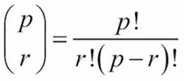
This binomial function involves computing three factorial values. It might make sense to use an @lru_cache decorator on a factorial function. A program that calculates a number of binomial values will not need to re-compute all of those factorials. For cases where similar values are computed repeatedly, the speedup can be impressive. For situations where the cached values are rarely reused, the overheads of maintaining the cached values outweigh any speedups.
When computing similar values repeatedly, we see the following:
· Naive Factorial 0.174
· Cached Factorial 0.046
· Cleared Cache Factorial 1.335
If we re-calculate the same binomial with the timeit module, we'll only really do the computation once, and return the same value the rest of the time; the cleared cache factorial shows the impact of clearing the cache before each calculation. The cache clearing operation—the cache_clear() function—introduces some overheads, making it appear more costly than it actually is. The moral of the story is that an lru_cache decorator is trivial to add. It often has a profound impact; but it may also have no impact, depending on the distribution of the actual data.
It's important to note that the cache is a stateful object. This design pushes the edge of the envelope on purely functional programming. A possible ideal is to avoid assignment statements and the associated changes of state. This concept of avoiding stateful variables is exemplified by a recursive function: the current state is contained in the argument values, and not in the changing values of variables. We've seen how tail-call optimization is an essential performance improvement to assure that this idealized recursion actually works nicely with the available processor hardware and limited memory budgets. In Python, we do this tail-call optimization manually by replacing the tail recursions with a for loop. Caching is a similar kind of optimization: we'll implement it manually as needed.
In principle, each call to a function with an LRU cache has two results: the expected result and a new cache object which should be used for all future requests. Pragmatically, we encapsulate the new cache object inside the decorated version of the fibc() function.
Caching is not a panacea. Applications that work with float values might not benefit much from memoization because all floats differ by small amounts. The least-significant bits of a float value are sometimes just random noise which prevents the exact equality test in the lru_cache decorator from working.
We'll revisit this in Chapter 16, Optimizations and Improvements. We'll look at some additional ways to implement this.
Defining classes with total ordering
The total_ordering decorator is helpful for creating new class definitions that implement a rich set of comparison operators. This might apply to numeric classes that subclass numbers.Number. It may also apply to semi-numeric classes.
As an example of a semi-numeric class, consider a playing card. It has a numeric rank and a symbolic suit. The rank matters only when doing simulations of some games. This is particularly important when simulating casino Blackjack. Like numbers, cards have an ordering. We often sum the point values of each card, making them number-like. However, multiplication of card × card doesn't really make any sense.
We can almost emulate a playing card with a namedtuple() function as follows:
Card1 = namedtuple("Card1", ("rank", "suit"))
This suffers from a profound limitation: all comparisons include both a rank and a suit by default. This leads to the following awkward 'margin-top:6.0pt;margin-right:29.0pt;margin-bottom: 6.0pt;margin-left:29.0pt;line-height:normal'>>>> c2s= Card1(2, '\u2660')
>>> c2h= Card1(2, '\u2665')
>>> c2h == c2s
False
This doesn't work well for Blackjack. It's unsuitable for certain Poker simulations also.
We'd really prefer the cards to be compared only by their rank. Following is a much more useful class definition. We'll show this in two parts. The first part defines the essential attributes:
@total_ordering
class Card(tuple):
__slots__ = ()
def __new__( class_, rank, suit ):
obj= tuple.__new__(Card, (rank, suit))
return obj
def __repr__(self):
return "{0.rank}{0.suit}".format(self)
@property
def rank(self):
return self[0]
@property
def suit(self):
return self[1]
This class extends the tuple class; it has no additional slots, thereby making it immutable. We've overridden the __new__() method so that we can seed initial values of a rank and a suit. We've provided a __repr__() method to print a string representation of a Card. We've provided two properties to extract a rank and a suit using attribute names.
The rest of the class definition shows how we can define just two comparisons:
def __eq__(self, other):
if isinstance(other,Card):
return self.rank == other.rank
elif isinstance(other,Number):
return self.rank == other
def __lt__(self, other):
if isinstance(other,Card):
return self.rank < other.rank
elif isinstance(other,Number):
return self.rank < other
We've defined the __eq__() and __lt__() functions. The @total_ordering decorator handles the construction of all other comparisons. In both cases, we've allowed comparisons between cards and also between a card and a number.
First, we get proper comparison of only the ranks as follows:
>>> c2s= Card(2, '\u2660')
>>> c2h= Card(2, '\u2665')
>>> c2h == c2s
True
>>> c2h == 2
True
We can use this class for a number of simulations with simplified syntax to compare ranks of cards. Further, we also have a rich set of comparison operators as follows:
>>> c2s= Card(2, '\u2660')
>>> c3h= Card(3, '\u2665')
>>> c4c= Card(4, '\u2663')
>>> c2s <= c3h < c4c
True
>>> c3h >= c3h
True
>>> c3h > c2s
True
>>> c4c != c2s
True
We didn't need to write all of the comparison method functions; they were generated by the decorator. The decorator's creation of operators isn't perfect. In our case, we've asked for comparisons with integers as well as between Card instances. This reveals some problems.
Operations like the c4c > 3 and 3 < c4c commands would raise TypeError exceptions. This is a limitation in what the total_ordering decorator can do. The problem rarely shows up in practice, since this kind of mixed-class coercion is relatively uncommon.
Object-oriented programming is not antithetical to functional programming. There is a realm in which the two techniques are complementary. Python's ability to create immutable objects works particularly well with functional programming techniques. We can easily avoid the complexities of stateful objects, but still benefit from encapsulation to keep related method functions together. It's particularly helpful to define class properties that involve complex calculations; this binds the calculations to the class definition, making the application easier to understand.
Defining number classes
In some cases, we might want to extend the numeric tower available in Python. A subclass of numbers.Number may simplify a functional program. We can, for example, isolate parts of a complex algorithm to the Number subclass definition, making other parts of the application simpler or clearer.
Python already offers a rich variety of numeric types. The built-in types of the int and float variables cover a wide variety of problem domains. When working with currency, the decimal.Decimal package handles this elegantly. In some cases, we might find thefractions.Fraction class to be more appropriate than the float variable.
When working with geographic data, for example, we might consider creating a subclass of float variable that introduces additional attributes for conversion between degrees of latitude (or longitude) and radians. The arithmetic operations in this subclass could be done ![]() to simplify calculations that move across the equator or the Greenwich meridian.
to simplify calculations that move across the equator or the Greenwich meridian.
Since Python Numbers class is intended to be immutable, ordinary functional design can be applied to all of the various method functions. The exceptional Python in-place special methods (for example, __iadd__() function) can be simply ignored.
When working with subclasses of Number, we have a fairly extensive volume of design considerations as follows:
· Equality testing and hash value calculation. The core features of hash calculation for numbers is documented in the 9.1.2 Notes for type implementors section of the Python Standard Library.
· The other comparison operators (often defined via @total_ordering decorator).
· The arithmetic operators: +, -, *, /, //, %, and **. There are special methods for the forward operations as well as additional methods for reverse type-matching. Given an expression like a-b, Python uses the type of a to attempt to locate an implementation of the __sub__() method function: effectively, the a.__sub__(b) method. If the class of the left-hand value, a in this case, doesn't have the method or returns the NotImplemented exception, then the right-hand value is examined to see if the b.__rsub__(a) method provides a result. There's an additional special case that applies when b's class is a subclass of a's class: this allows the subclass to override the left-hand side operation choice.
· The bit-fiddling operators: &, |, ^, >>, <<, and ~. These might not make sense for floating-point values; omitting these special methods might be the best design.
· Some additional functions like round(), pow(), and divmod() are implemented by numeric special method names. These might be meaningful for this class of numbers.
Chapter 7, Mastering Object-Oriented Python provides a detailed example of creating a new type of number. Visit the link for more details:
https://www.packtpub.com/application-development/mastering-object-oriented-python.
As we noted previously, functional programming and object-oriented programming can be complementary. We can easily define classes that follow functional programming design patterns. Adding new kinds of numbers is one example of leveraging Python's object-oriented features to create more readable functional programs.
Applying partial arguments with partial()
The partial() function leads to something called partial application. A partially applied function is a new function built from an old function and a subset of the required arguments. It is closely related to the concept of currying. Much of the theoretical background is not relevant here, since currying doesn't apply to the way Python functions are implemented. The concept, however, can lead us to some handy simplifications.
We can look at trivial examples as follows:
>>> exp2= partial(pow, 2)
>>> exp2(12)
4096
>>> exp2(17)-1
131071
We've created a function, exp2(y), which is the pow(2,y) function. The partial() function bounds the first positional parameter to the pow() function. When we evaluate the newly created exp2() function, we get values computed from the argument bound by thepartial() function, plus the additional argument provided to the exp2() function.
The bindings of positional parameters are handed in a strict left-to-right order. For functions that accept keyword parameters, these can also be provided when building the partially applied function.
We can also create this kind of partially applied function with a lambda form as follows:
exp2= lambda y: pow(2,y)
Neither is clearly superior. Measuring performance shows that the partial() function is a hair faster than a lambda form in the following manner:
· partial 0.37
· lambda 0.42
This is 0.05 seconds over 1,000,000 iterations: not a remarkable savings.
Since lambda forms have all of the capabilities of the partial() function, it seems that we can safely set this function aside as not being profoundly useful. We'll return to it in Chapter 14, The PyMonad Library, and look at how we can accomplish this with currying also.
Reducing sets of data with reduce()
The sum(), len(), max(), and min() functions are—in a way— all specializations of a more general algorithm expressed by the reduce() function. The reduce() function is a higher-order function that folds a function into each pair of items in an iterable.
A sequence object is given as follows:
d = [2, 4, 4, 4, 5, 5, 7, 9]
The function, reduce(lambda x,y: x+y, d), will fold in + operators to the list as follows:
2+4+4+4+5+5+7+9
Including () can show the effective grouping as follows:
((((((2+4)+4)+4)+5)+5)+7)+9
Python's standard interpretation of expressions involves a left-to-right evaluation of operators. The fold left isn't a big change in meaning.
We can also provide an initial value as follows:
reduce(lambda x,y: x+y**2, iterable, 0)
If we don't, the initial value from the sequence is used as the initialization. Providing an initial value is essential when there's a map() function as well as a reduce() function. Following is how the right answer is computed with an explicit 0 initializer:
0+ 2**2+ 4**2+ 4**2+ 4**2+ 5**2+ 5**2+ 7**2+ 9**2
If we omit the initialization of 0, and the reduce() function uses the first item as an initial value, we get the following wrong answer:
2+ 4**2+ 4**2+ 4**2+ 5**2+ 5**2+ 7**2+ 9**2
We can define a number of built-in reductions using the reduce() higher-order function as follows:
sum2= lambda iterable: reduce(lambda x,y: x+y**2, iterable, 0)
sum= lambda iterable: reduce(lambda x, y: x+y, iterable)
count= lambda iterable: reduce(lambda x, y: x+1, iterable, 0)
min= lambda iterable: reduce(lambda x, y: x if x < y else y, iterable)
max= lambda iterable: reduce(lambda x, y: x if x > y else y, iterable)
The sum2() reduction function is the sum of squares, useful for computing standard deviation of a set of samples. This sum() reduction function mimics the built-in sum() function. The count() reduction function is similar to the len() function, but it can work on an iterable, where the len() function can only work on a materialized collection object.
The min() and max() functions mimic the built-in reductions. Because the first item of the iterable is used for initialization, these two functions will work properly. If we provided any initial value to these reduce() functions, we might incorrectly use a value that never occurred in the original iterable.
Combining map() and reduce()
We can see how to build higher-order functions around these simple definitions. We'll show a simplistic map-reduce function that combines the map() and reduce() functions as follows:
def map_reduce(map_fun, reduce_fun, iterable):
return reduce(reduce_fun, map(map_fun, iterable))
We've created a composite function from the map() and reduce() functions that take three arguments: the mapping, the reduction operation, and the iterable or sequence to process.
We can build a sum-squared reduction using the map() and reduce() functions separately as follows:
def sum2_mr(iterable):
return map_reduce(lambda y: y**2, lambda x,y: x+y, iterable)
In this case, we've used the lambda y: y**2 parameter as a mapping to square each value. The reduction is simply lambda x,y: x+y parameter. We don't need to explicitly provide an initial value because the initial value will be the first item in the iterable after the map()function has squared it.
The lambda x,y: x+y parameter is merely the + operator. Python offers all of the arithmetic operators as short functions in the operator module. Following is how we can slightly simplify our map-reduce operation:
import operator
def sum2_mr2(iterable):
return map_reduce(lambda y: y**2, operator.add, iterable)
We've used the operator.add method to sum our values instead of the longer lambda form.
Following is how we can count values in an iterable:
def count_mr(iterable):
return map_reduce(lambda y: 1, operator.add, iterable)
We've used the lambda y: 1 parameter to map each value to a simple 1. The count is then a reduce() function using the operator.add method.
The general-purpose reduce() function allows us to create any species of reduction from a large dataset to a single value. There are some limitations, however, on what we should do with the reduce() function.
We should avoid executing commands such as the following:
reduce(operator.add, ["1", ",", "2", ",", "3"], "")
Yes, it works. However, the "".join(["1", ",", "2", ",", "3"]) method is considerably more efficient. We measured 0.23 seconds per million to do the "".join() function versus 0.69 seconds to do the reduce() function.
Using reduce() and partial()
Note
The sum() function can be seen as the partial(reduce, operator.add) method. This, too, gives us a hint as to how we can create other mappings and other reductions. We can, indeed, define all of the commonly used reductions as partials instead of lambdas.
Following are two examples:
sum2= partial(reduce, lambda x,y: x+y**2)
count= partial(reduce, lambda x,y: x+1)
We can now use these functions via the sum2(some_data) or the count(some_iter) method. As we noted previously, it's not clear how much benefit this has. It's possible that a particularly complex calculation can be explained simply with functions like this.
Using map() and reduce() to sanitize raw data
When doing data cleansing, we'll often introduce filters of various degrees of complexity to exclude invalid values. We may also include a mapping to sanitize values in the cases where a valid but improperly formatted value can be replaced with a valid but proper value.
We might produce the following output:
def comma_fix(data):
try:
return float(data)
except ValueError:
return float(data.replace(",", ""))
def clean_sum(cleaner, data):
return reduce(operator.add, map(cleaner, data))
We've defined a simple mapping, the comma_fix() class, that will convert data from a nearly correct format into a usable floating-point value.
We've also defined a map-reduce that applies a given cleaner function, the comma_fix() class, in this case, to the data before doing a reduce() function using the operator.add method.
We can apply the previously described function as follows:
>>> d = ('1,196', '1,176', '1,269', '1,240', '1,307', ... '1,435', '1,601', '1,654', '1,803', '1,734')
>>> clean_sum(comma_fix, d)
14415.0
We've cleaned the data, by fixing the commas, as well as computed a sum. The syntax is very convenient for combining these two operations.
We have to be careful, however, of using the cleaning function more than once. If we're also going to compute a sum of squares, we really should not execute the following command:
comma_fix_squared = lambda x: comma_fix(x)**2
If we use the clean_sum(comma_fix_squared, d) method as part of computing a standard deviation, we'll do the comma-fixing operation twice on the data: once to compute the sum and once to compute the sum of squares. This is a poor design; caching the results with an lru_cache decorator can help. Materializing the sanitized intermediate values as a temporary tuple object is probably better.
Using groupby() and reduce()
A common requirement is to summarize data after partitioning it into groups. We can use a defaultdict(list) method to partition data. We can then analyze each partition separately. In Chapter 4, Working with Collections, we looked at some ways to group and partition. In Chapter 8, The Itertools Module, we looked at others.
Following is some sample data that we need to analyze:
>>> data = [('4', 6.1), ('1', 4.0), ('2', 8.3), ('2', 6.5), ... ('1', 4.6), ('2', 6.8), ('3', 9.3), ('2', 7.8), ('2', 9.2), ... ('4', 5.6), ('3', 10.5), ('1', 5.8), ('4', 3.8), ('3', 8.1), ... ('3', 8.0), ('1', 6.9), ('3', 6.9), ('4', 6.2), ('1', 5.4), ... ('4', 5.8)]
We've got a sequence of raw data values with a key and a measurement for each key.
One way to produce usable groups from this data is to build a dictionary that maps a key to a list of members in this group as follows:
from collections import defaultdict
def partition(iterable, key=lambda x:x):
"""Sort not required."""
pd = defaultdict(list)
for row in iterable:
pd[key(row)].append(row)
for k in sorted(pd):
yield k, iter(pd[k])
This will separate each item in the iterable into individual groups. The key() function is used to extract a key value from each item. This key is used to append each item to a list in the pd dictionary. The resulting value of this function matches the results of theitertools.groupby() function: it's an iterable sequence of the (group key, iterator) pairs.
Following is the same feature done with the itertools.groupby() function:
def partition_s(iterable, key= lambda x:x):
"""Sort required"""
return groupby(iterable, key)
We can summarize the grouped data as follows:
mean= lambda seq: sum(seq)/len(seq)
var= lambda mean, seq: sum( (x-mean)**2/mean for x in seq)
def summarize( key_iter ):
key, item_iter= key_iter
values= tuple((v for k,v in item_iter))
μ= mean(values)
return key, μ, var(μ, values)
The results of the partition() functions will be a sequence of (key, iterator) two tuples. We'll separate the key from the item iterator. Each item in the item iterator is one of the original objects in the source data; these are (key, value) pairs; we only want the values, and so we've used a simple generator expression to separate the source keys from the values.
We can also execute the following command to pick the second item from each of the two tuples:
map(snd, item_iter)
This requires the snd= lambda x: x[1] method.
We can use the following command to apply the summarize() function to each partition:
>>> partition1= partition(list(data), key=lambda x:x[0])
>>> groups= map(summarize, partition1)
The alternative commands are as follows:
>>> partition2= partition_s(sorted(data), key=lambda x:x[0])
>>> groups= map(summarize, partition2)
Both will provide us summary values for each group. The resulting group statistics look as follows:
1 5.34 0.93
2 7.72 0.63
3 8.56 0.89
4 5.5 0.7
The variance can be used as part of a ![]() test to determine if the null hypothesis holds for this data. The null hypothesis asserts that there's nothing to see; the variance in the data is essentially random. We can also compare the data between the four groups to see if the various means are consistent with the null hypothesis or there is some statistically significant variation.
test to determine if the null hypothesis holds for this data. The null hypothesis asserts that there's nothing to see; the variance in the data is essentially random. We can also compare the data between the four groups to see if the various means are consistent with the null hypothesis or there is some statistically significant variation.
Summary
In this chapter, we've looked at a number of functions in the functools module. This library module provides a number of functions that help us create sophisticated functions and classes.
We've looked at the @lru_cache function as a way to boost certain types of applications with frequent re-calculations of the same values. This decorator is of tremendous value for certain kinds of functions that take the integer or the string argument values. It can reduce processing by simply implementing memoization.
We looked at the @total_ ordering function as a decorator to help us build objects that support rich ordering comparisons. This is at the fringe of functional programming, but is very helpful when creating new kinds of numbers.
The partial() function creates a new function with the partial application of argument values. As an alternative, we can build a lambda with similar features. The use case for this is ambiguous.
We also looked at the reduce() function as a higher-order function. This generalizes reductions like the sum() function. We'll use this function in several examples in the later chapters. This fits logically with the filter() and map() functions as an important higher-order function.
In the next chapters, we'll look at how we can build higher-order functions using decorators. These higher-order functions can lead to slightly simpler and clearer syntax. We can use decorators to define an isolated aspect that we need to incorporate into a number of other functions or classes.
All materials on the site are licensed Creative Commons Attribution-Sharealike 3.0 Unported CC BY-SA 3.0 & GNU Free Documentation License (GFDL)
If you are the copyright holder of any material contained on our site and intend to remove it, please contact our site administrator for approval.
© 2016-2026 All site design rights belong to S.Y.A.