Functional Python Programming (2015)

Chapter 16. Optimizations and Improvements

In this chapter, we'll look at a few optimizations that we can make to create high performance functional programs. We'll expand on the @lru_cache decorator from Chapter 10, The Functools Module. We have a number of ways to implement the memoization algorithm. We'll also discuss how to write our own decorators. More importantly, we'll see how we use a Callable object to cache memoized results.

We'll also look at some optimization techniques that were presented in Chapter 6, Recursions and Reductions. We'll review the general approach to tail recursion optimization. For some algorithms, we can combine memoization with a recursive implementation and achieve good performance. For other algorithms, memoization isn't really very helpful and we have to look elsewhere for performance improvements.

In most cases, small changes to a program will lead to small improvements in performance. Replacing a function with a lambda object will have a tiny impact on performance. If we have a program that is unacceptably slow, we often have to locate a completely new algorithm or data structure. Some algorithms have bad "big-O" complexity; nothing will make them magically run faster.

One place to start is http://www.algorist.com. This is a resource that may help to locate better algorithms for a given problem.

Memoization and caching

As we saw in Chapter 10, The Functools Module, many algorithms can benefit from memoization. We'll start with a review of some previous examples to characterize the kinds of functions that can be helped with memoization.

In Chapter 6, Recursions and Reductions, we looked at a few common kinds of recursions. The simplest kind of recursion is a tail recursion with arguments that can be easily matched to values in a cache. If the arguments are integers, strings, or materialized collections, then we can compare arguments quickly to determine if the cache has a previously computed result.

We can see from these examples that integer numeric calculations such as computing factorial or locating a Fibonacci number will be obviously improved. Locating prime factors and raising integers to powers are more examples of numeric algorithms that apply to integer values.

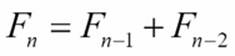
When we looked at the recursive version of a Fibonacci number calculator, we saw that it contained two tail-call recursions. Here's the definition:

This can be turned into a loop, but the design change requires some thinking. The memoized version of this can be quite fast and doesn't require quite so much thinking to design.

The Syracuse function, shown in Chapter 6, Recursions and Reductions, is an example of the kind of function used to compute fractal values. It contains a simple rule that's applied recursively. Exploring the Collatz conjecture ("does the Syracuse function always lead to 1?") requires memoized intermediate results.

The recursive application of the Syracuse function is an example of a function with an "attractor," where the value is attracted to 1. In some higher dimensional functions, the attractor can be a line or perhaps a fractal. When the attractor is a point, memoization can help; otherwise, memoization may actually be a hindrance, since each fractal value is unique.

When working with collections, the benefits of caching may vanish. If the collection happens to have the same number of integer values, strings, or tuples, then there's a chance that the collection is a duplicate and time can be saved. However, if a calculation on a collection will be needed more than once, manual optimization is best: do the calculation once and assign the results to a variable.

When working with iterables, generator functions, and other lazy objects, caching of an overall object is essentially impossible. In these cases, memoization is not going to help at all.

Raw data that includes measurements often use floating point values. Since an exact equality comparison between floating point values may not work out well, memoizing intermediate results may not work out well either.

Raw data that includes counts, however, may benefit from memoization. These are integers, and we can trust exact integer comparisons to (potentially) save recalculating a previous value. Some statistical functions, when applied to counts, can benefit from using the fractions module instead of floating point values. When we replace x/y with the Fraction(x,y) method, we've preserved the ability to do exact value matching. We can produce the final result using the float(some_fraction) method.

Specializing memoization

The essential idea of memoization is so simple that it can be captured by the @lru_cache decorator. This decorator can be applied to any function to implement memoization. In some cases, we might be able to improve on the generic idea with something more specialized. There are a large number of potentially optimizable multivalued functions. We'll pick one here and look at another in a more complex case study.

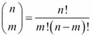
The binomial, , shows the number of ways n different things can be arranged in groups of size m. The value is as follows:

Clearly, we should cache the factorial calculations rather than redo all those multiplications. However, we may also benefit from caching the overall binomial calculation, too.

We'll create a Callable object that contains multiple internal caches. Here's a helper function that we'll need:

from functools import reduce

from operator import mul

prod = lambda x: reduce(mul, x)

The prod() function computes the product of an iterable of numbers. It's defined as a reduction using the * operator.

Here's a Callable object with two caches that uses this prod() function:

from collections.abc import Callable

class Binomial(Callable):

def __init__(self):

self.fact_cache= {}

self.bin_cache= {}

def fact(self, n):

if n not in self.fact_cache:

self.fact_cache[n] = prod(range(1,n+1))

return self.fact_cache[n]

def __call__(self, n, m):

if (n,m) not in self.bin_cache:

self.bin_cache[n,m] = self.fact(n)//(self.fact(m)*self.fact(n-m))

return self.bin_cache[n,m]

We created two caches: one for factorial values and one for binomial coefficient values. The internal fact() method uses the fact_cache attribute. If the value isn't in the cache, it's computed and added to the cache. The external __call__() method uses the bin_cacheattribute in a similar way: if a particular binomial has already been calculated, the answer is simply returned. If not, the internal fact() method is used to compute a new value.

We can use the preceding Callable class like this:

>>> binom= Binomial()

>>> binom(52,5)

2598960

This shows how we can create a Callable object from our class and then invoke the object on a particular set of arguments. There are a number of ways that a 52-card deck can be dealt into 5-card hands. There are 2.6 million possible hands.

Tail recursion optimizations

In Chapter 6, Recursions and Reductions, among many others, we looked at how a simple recursion can be optimized into a for loop. The general approach is this:

· Design the recursion. This means the base case and the recursive cases. For example, this is a definition of computing:

To design the recursion execute the following commands:

def fact(n):

if n == 0: return 1

else: return n*fact(n-1)

· If the recursion has a simple call at the end, replace the recursive case with a for loop. The command is as follows:

· def facti(n):

· if n == 0: return 1

· f= 1

· for i in range(2,n):

· f= f*i

· return f

When the recursion appears at the end of a simple function, it's described as a tail–call optimization. Many compilers will optimize this into a loop. Python—lacking this optimization in its compiler—doesn't do this kind of tail-call transformation.

This pattern is very common. Performing the tail-call optimization improves performance and removes any upper bound on the number of recursions that can be done.

Prior to doing any optimization, it's absolutely essential that the function already works. For this, a simple doctest string is often sufficient. We might use annotation on our factorial functions like this:

def fact(n):

"""Recursive Factorial

>>> fact(0)

1

>>> fact(1)

1

>>> fact(7)

5040

"""

if n == 0: return 1

else: return n*fact(n-1)

We added two edge cases: the explicit base case and the first item beyond the base case. We also added another item that would involve multiple iterations. This allows us to tweak the code with confidence.

When we have a more complex combination of functions, we might need to execute commands like this:

test_example="""

>>> binom= Binomial()

>>> binom(52,5)

2598960

"""

__test__ = {

"test_example": test_example,

}

The __test__ variable is used by the doctest.testmod() function. All of the values in the dictionary associated with the __test__ variable are examined for the doctest strings. This is a handy way to test features that come from compositions of functions. This is also called integration testing, since it tests the integration of multiple software components.

Having working code with a set of tests gives us the confidence to make optimizations. We can easily confirm the correctness of the optimization. Here's a popular quote that is used to describe optimization:

This appeared in the Bumper Sticker Computer Science chapter of More Programming Pearls, published by Addison-Wesley, Inc. What's important here is that we should only optimize code that's actually correct.

Optimizing storage

There's no general rule for optimization. We often focus on optimizing performance because we have tools like the Big O measure of complexity that show us whether or not an algorithm is an effective solution to a given problem. Optimizing storage is usually tackled separately: we can look at the steps in an algorithm and estimate the size of the storage required for the various storage structures.

In many cases, the two considerations are opposed. In some cases, an algorithm that has outstandingly good performance requires a large data structure. This algorithm can't scale without dramatic increases in the amount of storage required. Our goal is to design an algorithm that is reasonably fast and also uses an acceptable amount of storage.

We may have to spend time researching algorithmic alternatives to locate a way to make the space-time trade off properly. There are some common optimization techniques. We can often follow links from Wikipedia: http://en.wikipedia.org/wiki/Space–time_tradeoff.

One memory optimization technique we have in Python is to use an iterable. This has some properties of a proper materialized collection, but doesn't necessarily occupy storage. There are few operations (such as the len() function) that can't work on an iterable. For other operations, the memory saving feature can allow a program to work with very large collections.

Optimizing accuracy

In a few cases, we need to optimize the accuracy of a calculation. This can be challenging and may require some fairly advanced math to determine the limits on the accuracy of a given approach.

An interesting thing we can do in Python is replace floating point approximations with fractions.Fraction value. For some applications, this can create more accurate answers than floating point, because more bits are used for numerator and denominator than a floating point mantissa.

It's important to use decimal.Decimal values to work with currency. It's a common error to use a float value. When using a float value, additional noise bits are introduced because of the mismatch between Decimal values provided as input and the binary approximation used by floating point values. Using Decimal values prevents the introduction of tiny inaccuracies.

In many cases, we can make small changes to a Python application to switch from float values to Fraction or Decimal values. When working with transcendental functions, this change isn't necessarily beneficial. Transcendental functions—by definition—involve irrational numbers.

Reducing accuracy based on audience requirements

For some calculations, a fraction value may be more intuitively meaningful than a floating point value. This is part of presenting statistical results in a way that an audience can understand and take action on.

For example, the chi-squared test generally involves computing the comparison between actual values and expected values. We can then subject this comparison value to a test against the cumulative distribution function. When the expected and actual values have no particular relationship—we can call this a null relationship—the variation will be random; the value tends to be small. When we accept the null hypothesis, then we'll look elsewhere for a relationship. When the actual values are significantly different from the expected values, we may reject the null hypothesis. By rejecting the null hypothesis, we can explore further to determine the precise nature of the relationship.

The decision is often based on the table of the Cumulative Distribution Function (CDF) for selected values and given degrees of freedom. While the tabulated CDF values are mostly irrational values, we don't usually use more than two or three decimal places. This is merely a decision-making tool, there's no practical difference in meaning between 0.049 and 0.05.

A widely used probability is 0.05 for rejecting the null hypothesis. This is a Fraction object less than 1/20. When presenting data to an audience, it sometimes helps to characterize results as fractions. A value like 0.05 is hard to visualize. Describing a relationship has having 1 chance in 20 can help to characterize the likelihood of a correlation.

Case study – making a chi-squared decision

We'll look at a common statistical decision. The decision is described in detail at http://www.itl.nist.gov/div898/handbook/prc/section4/prc45.htm.

This is a chi-squared decision on whether or not data is distributed randomly. In order to make this decision, we'll need to compute an expected distribution and compare the observed data to our expectations. A significant difference means there's something that needs further investigation. An insignificant difference means we can use the null hypothesis that there's nothing more to study: the differences are simply random variation.

We'll show how we can process the data with Python. We'll start with some backstory—some details that are not part of the case study, but often features an Exploratory Data Analysis (EDA) application. We need to gather the raw data and produce a useful summary that we can analyze.

Within the production quality assurance operations, silicon wafer defect data is collected into a database. We might use SQL queries to extract defect details for further analysis. For example, a query could look like this:

SELECT SHIFT, DEFECT_CODE, SERIAL_NUMBER

FROM some tables;

The output from this query could be a CSV file with individual defect details:

shift,defect_code,serial_number

1,None,12345

1,None,12346

1,A,12347

1,B,12348

and so on. for thousands of wafers

We need to summarize the preceding data. We might summarize at the SQL query level using the COUNT and GROUP BY statements. We might also summarize at the Python application level. While a pure database summary is often described as being more efficient, this isn't always true. In some cases, a simple extract of raw data and a Python application to summarize can be faster than a SQL summary. If performance is important, both alternatives must be measured, rather than hoping that the database is fastest.

In some cases, we may be able to get summary data from the database efficiently. This summary must have three attributes: the shift, type of defect, and a count of defects observed. The summary data looks like this:

shift,defect_code,count

1,A,15

2,A,26

3,A,33

and so on.

The output will show all of the 12 combinations of shift and defect type.

In the next section, we'll focus on reading the raw data to create summaries. This is the kind of context in which Python is particularly powerful: working with raw source data.

We need to observe and compare shift and defect counts with an overall expectation. If the difference between observed counts and expected counts can be attributed to random fluctuation, we have to accept the null hypothesis that nothing interesting is going wrong. If, on the other hand, the numbers don't fit with random variation, then we have a problem that requires further investigation.

Filtering and reducing the raw data with a Counter object

We'll represent the essential defect counts as a collections.Counter parameter. We will build counts of defects by shift and defect type from the detailed raw data. Here's a function to read some raw data from a CSV file:

import csv

from collections import Counter

from types import SimpleNamespace

def defect_reduce(input):

rdr= csv.DictReader(input)

assert sorted(rdr.fieldnames) == ["defect_type", "serial_number", "shift"]

rows_ns = (SimpleNamespace(**row) for row in rdr)

defects = ((row.shift, row.defect_type) for row in rows_ns:

if row.defect_type)

tally= Counter(defects)

return tally

The preceding function will create a dictionary reader based on an open file provided via the input parameter. We've confirmed that the column names match the three expected column names. In some cases, we'll have extra columns in the file; in this case, the assertion will be something like all((c in rdr.fieldnames) for c in […]). Given a tuple of column names, this will assure that all of the required columns are present in the source. We can also use sets to assure that set(rdr.fieldnames) <= set([...]).

We created a types.SimpleNamespace parameter for each row. In the preceding example, the supplied column names are valid Python variable names that allow us to easily turn a dictionary into a namespace. In some cases, we'll need to map column names to Python variable names to make this work.

A SimpleNamespace parameter allows us to use slightly simpler syntax to refer to items within the row. Specifically, the next generator expression uses references such as row.shift and row.defect_type instead of the bulkier row['shift'] or row['defect_type']references.

We can use a more complex generator expression to do a map-filter combination. We'll filter each row to ignore rows with no defect code. For rows with a defect code, we're mapping an expression which creates a two tuple from the row.shift and row.defect_typereferences.

In some applications, the filter won't be a trivial expression such as row.defect_type. It may be necessary to write a more sophisticated condition. In this case, it may be helpful to use the filter() function to apply the complex condition to the generator expression that provides the data.

Given a generator that will produce a sequence of (shift, defect) tuples, we can summarize them by creating a Counter object from the generator expression. Creating this Counter object will process the lazy generator expressions, which will read the source file, extract fields from the rows, filter the rows, and summarize the counts.

We'll use the defect_reduce() function to gather and summarize the data as follows:

with open("qa_data.csv", newline="" ) as input:

defects= defect_reduce(input)

print(defects)

We can open a file, gather the defects, and display them to be sure that we've properly summarized by shift and defect type. Since the result is a Counter object, we can combine it with other Counter objects if we have other sources of data.

The defects value looks like this:

Counter({('3', 'C'): 49, ('1', 'C'): 45, ('2', 'C'): 34, ('3', 'A'): 33, ('2', 'B'): 31, ('2', 'A'): 26, ('1', 'B'): 21, ('3', 'D'): 20, ('3', 'B'): 17, ('1', 'A'): 15, ('1', 'D'): 13, ('2', 'D'): 5})

We have defect counts organized by shift and defect types. We'll look at alternative input of summarized data next. This reflects a common use case where data is available at the summary level.

Once we've read the data, the next step is to develop two probabilities so that we can properly compute expected defects for each shift and each type of defect. We don't want to divide the total defect count by 12, since that doesn't reflect the actual deviations by shift or defect type. The shifts may be more or less equally productive. The defect frequencies are certainly not going to be similar. We expect some defects to be very rare and others to be more common.

Reading summarized data

As an alternative to reading all of the raw data, we can look at processing only the summary counts. We want to create a Counter object similar to the previous example; this will have defect counts as a value with a key of shift and defect code. Given summaries, we simply create a Counter object from the input dictionary.

Here's a function that will read our summary data:

from collections import Counter

import csv

def defect_counts(source):

rdr= csv.DictReader(source)

assert rdr.fieldnames == ["shift", "defect_code", "count"]

convert = map(lambda d: ((d['shift'], d['defect_code']), int(d['count'])),

rdr)

return Counter(dict(convert))

We require an open file as the input. We'll create a csv.DictReader() function that helps parse the raw CSV data that we got from the database. We included an assert statement to confirm that the file really has the expected data.

We defined a lambda object that creates a two tuple with the key and the integer conversion of the count. The key is itself a two tuple with the shift and defect information. The result will be a sequence such as ((shift,defect), count), ((shift,defect), count), …). When we map the lambda to the DictReader parameter, we'll have a generator function that can emit the sequence of two tuples.

We will create a dictionary from the collection of two tuples and use this dictionary to build a Counter object. The Counter object can easily be combined with other Counter objects. This allows us to combine details acquired from several sources. In this case, we only have a single source.

We can assign this single source to the variable defects. The value looks like this:

Counter({('3', 'C'): 49, ('1', 'C'): 45, ('2', 'C'): 34, ('3', 'A'): 33, ('2', 'B'): 31, ('2', 'A'): 26,('1', 'B'): 21, ('3', 'D'): 20, ('3', 'B'): 17, ('1', 'A'): 15, ('1', 'D'): 13, ('2', 'D'): 5})

This matches the detail summary shown previously. The source data, however, was already summarized. This is often the case when data is extracted from a database and SQL is used to do group-by operations.

Computing probabilities from a Counter object

We need to compute the probabilities of defects by shift and defects by type. In order to compute the expected probabilities, we need to start with some simple sums. The first is the overall sum of all defects, which can be calculated by executing the following command:

total= sum(defects.values())

This is done directly from the values in the Counter object assigned to the defects variable. This will show that there are 309 total defects in the sample set.

We need to get defects by shift as well as defects by type. This means that we'll extract two kinds of subsets from the raw defect data. The "by-shift" extract will use just one part of the (shift,defect type) key in the Counter object. The "by-type" will use the other half of the key pair.

We can summarize by creating additional Counter objects extracted from the initial set of the Counter objects assigned to the defects variable. Here's the by-shift summary:

shift_totals= sum((Counter({s:defects[s,d]}) for s,d in defects), Counter())

We've created a collection of individual Counter objects that have a shift, s, as the key and the count of defects associated with that shift defects[s,d]. The generator expression will create 12 such Counter objects to extract data for all combinations of four defect types and three shifts. We'll combine the Counter objects with a sum() function to get three summaries organized by shift.

Note

We can't use the default initial value of 0 for the sum() function. We must provide an empty Counter() function as an initial value.

The type totals are created with an expression similar to the one used to create shift totals:

type_totals= sum((Counter({d:defects[s,d]}) for s,d in defects), Counter())

We created a dozen Counter objects using the defect type, d, as the key instead of shift type; otherwise, the processing is identical.

The shift totals look like this:

Counter({'3': 119, '2': 96, '1': 94})

The defect type totals look like this:

Counter({'C': 128, 'A': 74, 'B': 69, 'D': 38})

We've kept the summaries as Counter objects, rather than creating simple dict objects or possibly even list instances. We'll generally use them as simple dicts from this point forward. However, there are some situations where we will want proper Counter objects instead of reductions.

Alternative summary approaches

We've read the data and computed summaries in two separate steps. In some cases, we may want to create the summaries while reading the initial data. This is an optimization that might save a little bit of processing time. We could write a more complex input reduction that emitted the grand total, the shift totals, and the defect type totals. These Counter objects would be built one item at a time.

We've focused on using the Counter instances, because they seem to allow us flexibility. Any changes to the data acquisition will still create Counter instances and won't change the subsequent analysis.

Here's how we can compute the probabilities of defect by shift and by defect type:

from fractions import Fraction

P_shift = dict( (shift, Fraction(shift_totals[shift],total))

for shift in sorted(shift_totals))

P_type = dict((type, Fraction(type_totals[type],total)) for type in sorted(type_totals))

We've created two dictionaries: P_shift and P_type. The P_shift dictionary maps a shift to a Fraction object that shows the shift's contribution to the overall number of defects. Similarly, the P_type dictionary maps a defect type to a Fraction object that shows the type's contribution to the overall number of defects.

We've elected to use Fraction objects to preserve all of the precision of the input values. When working with counts like this, we may get probability values that make more intuitive sense to people reviewing the data.

We've elected to use dict objects because we've switched modes. At this point in the analysis, we're no longer accumulating details; we're using reductions to compare actual and observed data.

The P_shift data looks like this:

{'2': Fraction(32, 103), '3': Fraction(119, 309), '1': Fraction(94, 309)}

The P_type data looks like this:

{'B': Fraction(23, 103), 'C': Fraction(128, 309), 'A': Fraction(74, 309), 'D': Fraction(38, 309)}

A value such as 32/103 or 96/309 might be more meaningful to some people than 0.3106. We can easily get float values from Fraction objects, as we'll see later.

The shifts all seem to be approximately at the same level of defect production. The defect types vary, which is typical. It appears that the defect C is a relatively common problem, whereas the defect B is much less common. Perhaps the second defect requires a more complex situation to arise.

Computing expected values and displaying a contingency table

The expected defect production is a combined probability. We'll compute the shift defect probability multiplied by the probability based on defect type. This will allow us to compute all 12 probabilities from all combinations of shift and defect type. We can weight these with the observed numbers and compute the detailed expectation for defects.

Here's the calculation of expected values:

expected = dict(((s,t), P_shift[s]*P_type[t]*total) for t in P_type:for s in P_shift)

We'll create a dictionary that parallels the initial defects Counter object. This dictionary will have a sequence of two tuples with keys and values. The keys will be two tuples of shift and defect type. Our dictionary is built from a generator expression that explicitlyenumerates all combinations of keys from the P_shift and P_type dictionaries.

The value of the expected dictionary looks like this:

{('2', 'B'): Fraction(2208, 103), ('2', 'D'): Fraction(1216, 103),('3', 'D'): Fraction(4522, 309), ('2', 'A'): Fraction(2368, 103),('1', 'A'): Fraction(6956, 309), ('1', 'B'): Fraction(2162, 103),('3', 'B'): Fraction(2737, 103), ('1', 'C'): Fraction(12032, 309),('3', 'C'): Fraction(15232, 309), ('2', 'C'): Fraction(4096, 103),('3', 'A'): Fraction(8806, 309), ('1', 'D'): Fraction(3572, 309)}

Each item of the mapping has a key with shift and defect type. This is associated with a Fraction value based on the probability of defect based on shift times, the probability of a defect based on defect type times the overall number of defects. Some of the fractions are reduced, for example, a value of 6624/309 can be simplified to 2208/103.

Large numbers are awkward as proper fractions. Displaying large values as float values is often easier. Small values (such as probabilities) are sometimes easier to understand as fractions.

We'll print the observed and expected times in pairs. This will help us visualize the data. We'll create something that looks like the following to help summarize what we've observed and what we expect:

obs exp obs exp obs exp obs exp

15 22.51 21 20.99 45 38.94 13 11.56 94

26 22.99 31 21.44 34 39.77 5 11.81 96

33 28.50 17 26.57 49 49.29 20 14.63 119

74 69 128 38 309

This shows 12 cells. Each cell has values with the observed number of defects and an expected number of defects. Each row ends with the shift totals, and each column has a footer with the defect totals.

In some cases, we might export this data in CSV notation and build a spreadsheet. In other cases, we'll build an HTML version of the contingency table and leave the layout details to a browser. We've shown a pure text version here.

Here's a sequence of statements to create the contingency table shown previously:

print("obs exp"*len(type_totals))

for s in sorted(shift_totals):

pairs= ["{0:3d} {1:5.2f}".format(defects[s,t], float(expected[s,t])) for t in sorted(type_totals)]

print("{0} {1:3d}".format( "".join(pairs), shift_totals[s]))

footers= ["{0:3d}".format(type_totals[t]) for t in sorted(type_totals)]

print("{0} {1:3d}".format("".join(footers), total))

This spreads the defect types across each line. We've written enough obs exp column titles to cover all defect types. For each shift, we'll emit a line of observed and actual pairs, followed by a shift total. At the bottom, we'll emit a line of footers with just the defect type totals and the grand total.

A contingency table like this one helps us to visualize the comparison between observed and expected values. We can compute a chi-squared value for these two sets of values. This will help us decide if the data is random or if there's something that deserves further investigation.

Computing the chi-squared value

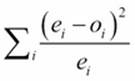The value is based on , where the e values are the expected values and the o values are the observed values.

We can compute the specified formula's value as follows:

diff= lambda e,o: (e-o)**2/e

chi2= sum(diff(expected[s,t], defects[s,t]) for s in shift_totals:

for t in type_totals

)

We've defined a small lambda to help us optimize the calculation. This allows us to execute the expected[s,t] and defects[s,t] attributes just once, even though the expected value is used in two places. For this dataset, the final value is 19.18.

There are a total of six degrees of freedom based on three shifts and four defect types. Since we're considering them independent, we get 2×3=6. A chi-squared table shows us that anything below 12.5916 would reflect 1 chance in 20 of the data being truly random. Since our value is 19.18, the data is unlikely to be random.

The cumulative distribution function for shows that a value of 19.18 has a probability of the order of 0.00387: about 4 chances in 1000 of being random. The next step is a follow-up study to discover the details of the various defect types and shifts. We'll need to see which independent variable has the biggest correlation with defects and continue the analysis.

Instead of following up with this case study, we'll look at a different and interesting calculation.

Computing the chi-squared threshold

The essence of the test is a threshold value based on the number of degrees of freedom and the level of uncertainty we're willing to entertain in accepting or rejecting the null hypothesis. Conventionally, we're advised to use a threshold around 0.05 (1/20) to reject the null hypothesis. We'd like there to be only 1 chance in 20 that the data is simply random and it appears meaningful. In other words, we'd like there to be 19 chances in 20 that the data reflects simple random variation.

The chi-squared values are usually provided in tabular form because the calculation involves a number of transcendental functions. In some cases, libraries will provide the cumulative distribution function, allowing us to compute a value rather than look one up on tabulation of important values.

The cumulative distribution function for a value, x, and degrees of freedom, f, is defined as follows:

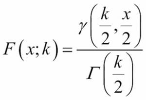
It's common to the probability of being random as . That is, if p > 0.05, the data can be understood as random; the null hypothesis is true.

This requires two calculations: the incomplete gamma function, , and the complete gamma function, . These can involve some fairly complex math. We'll cut some corners and implement two pretty-good approximations that are narrowly focused on just this problem. Each of these functions will allow us to look at functional design issues.

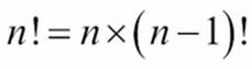
Both of these functions will require a factorial calculation, . We've seen several variations on the fractions theme. We'll use the following one:

@lru_cache(128)

def fact(k):

if k < 2: return 1

return reduce(operator.mul, range(2, int(k)+1))

This is : a product of numbers from 2 to k (inclusive). We've omitted the unit test cases.

Computing the partial gamma value

The partial gamma function has a simple series expansion. This means that we're going to compute a sequence of values and then do a sum on those values. For more information, visit http://dlmf.nist.gov/8.

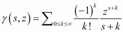
This series will have a sequence of terms that—eventually—become too small to be relevant. The calculation will yield alternating signs:

The sequence of terms looks like this with s=1 and z=2:

2/1, -2/1, 4/3, -2/3, 4/15, -4/45, ..., -2/638512875

At some point, each additional term won't have any significant impact on the result.

When we look back at the cumulative distribution function, , we can consider working with fractions.Fraction values. The degrees of freedom, k, will be an integer divided by 2. The value, x, may be either a Fraction or a float value; it will rarely be a simple integer value.

When evaluating the terms of , the value of will involve integers and can be represented as a proper Fraction value. The value of could be a Fraction or float value; it will lead to irrational values when is not an integer value. The value of will be a proper Fraction value, sometimes it will have the integer values, and sometimes it will have values that involve 1/2.

The use of Fraction value here—while possible—doesn't seem to be helpful because there will be an irrational value computed. However, when we look at the complete gamma function given here, we'll see that Fraction values are potentially helpful. In this function, they're merely incidental.

Here's an implementation of the previously explained series expansion:

def gamma(s, z):

def terms(s, z):

for k in range(100):

t2= Fraction(z**(s+k))/(s+k)

term= Fraction((-1)**k,fact(k))*t2

yield term

warnings.warn("More than 100 terms")

def take_until(function, iterable):

for v in iterable:

if function(v): return

yield v

ε= 1E-8

return sum(take_until(lambda t:abs(t) < ε, terms(s, z)))

We defined a term() function that will yield a series of terms. We used a for statement with an upper limit to generate only 100 terms. We could have used the itertools.count() function to generate an infinite sequence of terms. It seems slightly simpler to use a loop with an upper bound.

We computed the irrational value and created a Fraction value from this value by itself. If the value for z is also a Fraction value and not a float value then, the value for t2 will be a Fraction value. The value for term() function will then be a product of twoFraction objects.

We defined a take_until() function that takes values from an iterable, until a given function is true. Once the function becomes true, no more values are consumed from the iterable. We also defined a small threshold value, ε, of . We'll take values from theterm() function until the values are less than ε. The sum of these values is an approximation to the partial gamma function.

Here are some test cases we can use to confirm that we're computing this properly:

·

·

·

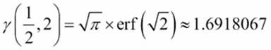
The error function, erf(), is another interesting function. We won't look into it here because it's available in the Python math library.

Our interest is narrowly focused on the chi-squared distribution. We're not generally interested in the incomplete gamma function for other mathematical purposes. Because of this, we can narrow our test cases to the kinds of values we expect to be using. We can also limit the accuracy of the results. Most chi-squared tests involve three digits of precision. We've shown seven digits in the test data, which is more than we might properly need.

Computing the complete gamma value

The complete gamma function is a bit more difficult. There are a number of different approximations. For more information, visit http://dlmf.nist.gov/5. There's a version available in the Python math library. It represents a broadly useful approximation that is designed for many situations.

We're not actually interested in a general implementation of the complete gamma function. We're interested in just two special cases: integer values and halves. For these two special cases, we can get exact answers, and don't need to rely on an approximation.

For integer values, . The gamma function for integers can rely on the factorial function we defined previously.

For halves, there's a special form:

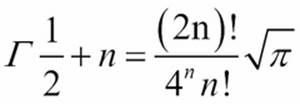
This includes an irrational value, so we can only represent this approximately using float or Fraction objects.

Since the chi-squared cumulative distribution function only uses the following two features of the complete gamma function, we don't need a general approach. We can cheat and use the following two values, which are reasonably precise.

If we use proper Fraction values, then we can design a function with a few simple cases: an integer value, a Fraction value with 1 in the denominator, and a Fraction value with 2 in the denominator. We can use the Fraction value as follows:

sqrt_pi = Fraction(677622787, 382307718)

def Gamma_Half(k):

if isinstance(k,int):

return fact(k-1)

elif isinstance(k,Fraction):

if k.denominator == 1:

return fact(k-1)

elif k.denominator == 2:

n = k-Fraction(1,2)

return fact(2*n)/(Fraction(4**n)*fact(n))*sqrt_pi

raise ValueError("Can't compute Γ({0})".format(k))

We called the function Gamma_Half to emphasize that this is only appropriate for whole numbers and halves. For integer values, we'll use the fact() function that was defined previously. For Fraction objects with a denominator of 1, we'll use the same fact() definition:.

For the cases where the denominator is 2, we can use the more complex "closed form" value. We used an explicit Fraction() function for the value . We've also provided a Fraction approximation for the irrational value .

Here are some test cases:

·

·

·

·

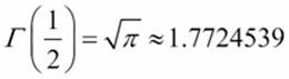
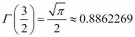
These can also be shown as proper Fraction values. The irrational values lead to large, hard-to-read fractions. We can use something like this:

>>> g= Gamma_Half(Fraction(3,2))

>>> g.limit_denominator(2000000)

Fraction(291270, 328663)

This provides a value where the denominator has been limited to be in the range of 1 to 2 million; this provides pleasant-looking six-digit numbers that we can use for unit test purposes.

Computing the odds of a distribution being random

Now that we have the incomplete gamma function, gamma, and complete gamma function, Gamma_Half, we can compute the CDF values. The CDF value shows us the odds of a given value being random or having some possible correlation.

The function itself is quite small:

def cdf(x, k):

"""X² cumulative distribution function.

:param x: X² value -- generally sum (obs[i]-exp[i])**2/exp[i]

for parallel sequences of observed and expected values.:param k: degrees of freedom >= 1; generally len(data)-1

"""

return 1-gamma(Fraction(k,2), Fraction(x/2))/Gamma_Half(Fraction(k,2))

We included some docstring comments to clarify the parameters. We created proper Fraction objects from the degrees of freedom and the chi-squared value, x. When converting a float value to a Fraction object, we'll create a very large fractional result with a large number of entirely irrelevant digits.

We can use Fraction(x/2).limit_denominator(1000) to limit the size of the x/2 Fraction method to a respectably small number of digits. This will compute a correct CDF value, but won't lead to gargantuan fractions with dozens of digits.

Here are some sample data called from a table of . Visit http://en.wikipedia.org/wiki/Chi-squared_distribution for more information.

To compute the correct CDF values execute the following commands:

>>> round(float(cdf(0.004, 1)), 2)

0.95

>>> cdf(0.004, 1).limit_denominator(100)

Fraction(94, 99)

>>> round(float(cdf(10.83, 1)), 3)

0.001

>>> cdf(10.83, 1).limit_denominator(1000)

Fraction(1, 1000)

>>> round(float(cdf(3.94, 10)), 2)

0.95

>>> cdf(3.94, 10).limit_denominator(100)

Fraction(19, 20)

>>> round(float(cdf(29.59, 10)), 3)

0.001

>>> cdf(29.59, 10).limit_denominator(10000)

Fraction(8, 8005)

Given and a number of degrees of freedom, our CDF function produces the same results as a widely used table of values.

Here's an entire row from a table, computed with a simple generator expression:

>>> chi2= [0.004, 0.02, 0.06, 0.15, 0.46, 1.07, 1.64, 2.71, 3.84, 6.64, 10.83]

>>> act= [round(float(x), 3) for x in map(cdf, chi2, [1]*len(chi2))]

>>> act

[0.95, 0.888, 0.806, 0.699, 0.498, 0.301, 0.2, 0.1, 0.05, 0.01, 0.001]

The expected values are as follows:

[0.95, 0.90, 0.80, 0.70, 0.50, 0.30, 0.20, 0.10, 0.05, 0.01, 0.001]

We have some tiny discrepancies in the third decimal place.

What we can do with this is get a probability from a value. From our example shown previously, the 0.05 probability for six degrees of freedom has a value 12.5916

>>> round(float(cdf(12.5916, 6)), 2)

0.05

The actual value we got for in the example was 19.18. Here's the probability that this value is random:

>>> round(float(cdf(19.18, 6)), 5)

0.00387

This probability is 3/775, with the denominator limited to 1000. Those are not good odds of the data being random.

Summary

In this chapter, we looked at three optimization techniques. The first technique involves finding the right algorithm and data structure. This has more impact on performance than any other single design or programming decision. Using the right algorithm can easily reduce runtimes from minutes to fractions of a second. Changing a poorly used sequence to a properly used mapping, for example, may reduce run time by a factor of 200.

We should generally optimize all of our recursions to be loops. This will be faster in Python and it won't be stopped by the call stack limit that Python imposes. There are many examples of how recursions are flattened into loops in other chapters, primarily, Chapter 6, Recursions and Reductions. Additionally, we may be able to improve performance in two other ways. First, we can apply memoization to cache results. For numeric calculations, this can have a large impact; for collections, the impact may be less. Secondly, replacing large materialized data objects with iterables may also improve performance by reducing the amount of memory management required.

In the case study presented in this chapter, we looked at the advantage of using Python for exploratory data analysis—the initial data acquisition including a little bit of parsing and filtering. In some cases, a significant amount of effort is required to normalize data from various sources. This is a task at which Python excels.

The calculation of a value involved three sum() functions: two intermediate generator expressions, and a final generator expression to create a dictionary with expected values. A final sum() function created the statistic. In under a dozen expressions, we created a sophisticated analysis of data that will help us accept or reject the null hypothesis.

We also evaluated some complex statistical functions: the incomplete and the complete gamma function. The incomplete gamma function involves a potentially infinite series; we truncated this and summed the values. The complete gamma function has some potential complexity, but it doesn't happen to apply in our case.

Using a functional approach, we can write succinct and expressive programs that accomplish a great deal of processing. Python isn't a properly functional programming language. For example, we're required to use some imperative programming techniques. This limitation forces away from purely functional recursions. We gain some performance advantage, since we're forced to optimize tail recursions into explicit loops.

We also saw numerous advantages of adopting Python's hybrid style of functional programming. In particular, the use of Python's higher order functions and generator expressions give us a number of ways to write high performance programs that are often quite clear and simple.