Algorithms in a Nutshell: A Practical Guide (2016)

Appendix A. Benchmarking

Each algorithm in this book is accompanied by data about its performance. Because it’s important to use the right benchmarks to get accurate performance, we present our infrastructure to evaluate algorithm performance in this appendix. This should also help to address any questions or doubts you might have concerning the validity of our approach. We try to explain the precise means by which empirical data is computed, in order to enable you both to verify that the results are accurate and to understand where the assumptions are appropriate given the context in which the algorithm is intended to be used.

There are numerous ways by which algorithms can be analyzed. Chapter 2 presented a theoretical, formal treatment, introducing the concepts of worst-case and average-case analysis. These theoretic results can be empirically evaluated in some cases, but not all. For example, consider evaluating the performance of an algorithm to sort 20 numbers. There are 2.43*10¹⁸ permutations of these 20 numbers, and we cannot simply exhaustively evaluate each of these permutations to compute the average case. Additionally, we cannot compute the average by measuring the time to sort all of these permutations. We must rely on statistical measures to assure ourselves we have properly computed the expected performance time of the algorithm.

Statistical Foundation

This chapter focuses on essential points for evaluating the performance of algorithms. Interested readers should consult any of the large number of available textbooks on statistics for more information on the relevant statistical information used to produce the empirical measurements in this book.

To compute the performance of an algorithm, we construct a suite of T independent trials for which the algorithm is executed. Each trial is intended to execute an algorithm on an input problem of size n. Some effort is made to ensure these trials are all reasonably equivalent for the algorithm. When the trials are actually identical, the intent of the trial is to quantify the variance of the underlying implementation of the algorithm. This may be suitable, for example, if it is too costly to compute a large number of independent equivalent trials.

The suite is executed and millisecond-level timings are taken before and after the observable behavior. When the code is written in Java, the system garbage collector is invoked immediately prior to launching the trial; although this effort can’t guarantee that the garbage collector does not execute during the trial, it may reduce this risk of spending extra time unrelated to the algorithm. From the full set of T recorded times, the best and worst performing times are discarded as being “outliers.” The remaining T − 2 time records are averaged, and a standard deviation is computed using the following formula:

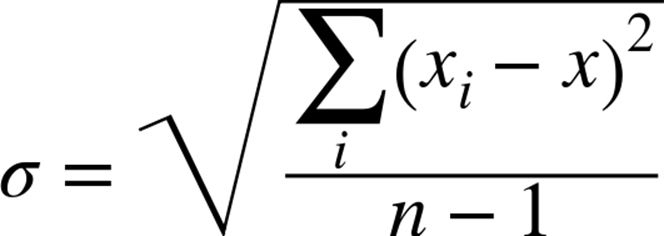
where x_i is the time for an individual trial and x is the average of the T − 2 trials. Note here that n is equal to T − 2, so the denominator within the square root is T − 3. Calculating averages and standard deviations will help predict future performance, based on Table A-1, which shows the probability (between 0 and 1) that the actual value will be within the range [x – k*σ, x + k*σ], where σ represents the standard deviation computed in the equation just shown. The probability values become confidence intervals that declare the confidence we have in a prediction.

For example, in a randomized trial, it is expected that 68.27% of the time the result will fall within the range [x–σ, x+σ].

When reporting results, we never present numbers with greater than four decimal digits of accuracy, so we don’t give the mistaken impression that we believe the accuracy of our numbers extends any farther. This process will convert a computation such as 16.897986 into the reported number 16.8980.

Example

Assume we wanted to benchmark the addition of the numbers from 1 to n. An experiment is designed to measure the times for n = 8,000,000 to n = 16,000,000 in increments of two million. Because the problem is identical for n and doesn’t vary, we execute for 30 trials to eliminate as much variability as possible.

The hypothesis is that the time to complete the sum will vary directly in relation to n. We show three programs that solve this problem—in Java, C, and Python—and present the benchmark infrastructure by showing how it is used.

Java Benchmarking Solutions

On Java test cases, the current system time (in milliseconds) is determined immediately prior to, and after, the execution of interest. The code in Example A-1 measures the time it takes to complete the task. In a perfect computer, the 30 trials should all require exactly the same amount of time. Of course, this is unlikely to happen, because modern operating systems have numerous background processing tasks that share the same CPU on which the performance code executes.

Example A-1. Java example to time execution of task

public class Main {

public static void main (String[] args) {

TrialSuite ts = new TrialSuite();

for (long len = 8000000; len <= 16000000; len += 2000000) {

for (int i = 0; i < 30; i++) {

System.gc();

long now = System.currentTimeMillis();

/** Task to be timed. */

long sum = 0;

for (int x = 1; x <= len; x++) {

sum += x;

}

long end = System.currentTimeMillis();

ts.addTrial(len, now, end);

}

}

System.out.println (ts.computeTable());

}

}

The TrialSuite class stores trials by their size. After all the trials have been added to the suite, the resulting table is computed. To do this, the running times are added together to find the total sum, minimum value, and maximum value. As described earlier, the minimum and maximum values are removed from the set when computing the average and standard deviation.

Linux Benchmarking Solutions

For C test cases, we developed a benchmarking library to be linked with the code to test. In this section, we briefly describe the essential aspects of the timing code and refer the interested reader to the code repository for the full source.

Primarily created for testing sort routines, the C-based infrastructure can be linked to existing source code. The timing API takes over responsibility for parsing the command-line arguments:

usage: timing [-n NumElements] [-s seed] [-v] [OriginalArguments]

-n declares the problem size [default: 100,000]

-v verbose output [default: false]

-s # set the seed for random values [default: no seed]

-h print usage information

The timing library assumes a problem will be attempted whose input size is defined by the [-n] flag. To produce repeatable trials, the random seed can be set with [-s seed]. To link with the timing library, a test case provides the following functions:

void problemUsage()

Report to the console the set of [OriginalArguments] supported by the specific code. Note that the timing library parses the declared timing parameters, and remaining arguments are passed along to the prepareInput function.

void prepareInput (int size, int argc, char **argv)

For some problems, this function is responsible for building the input set to be processed within the execute method. Note that this information is not passed directly to execute via a formal argument, but instead is stored as a static variable within the test case.

void postInputProcessing()

If any validation is needed after the input problem is solved, that code can execute here.

void execute()

This method contains the body of code to be timed. Because the code is run once as part of the evaluation time, it can have a small impact on the reported time. When the execute method is empty, the overhead is considered to have no impact on the overall reporting.

The test case in Example A-2 shows the code task for the addition example.

Example A-2. Task describing addition of n numbers

extern int numElements; /* size of n */

void problemUsage() { /* none */ }

void prepareInput() { /* none */ }

void postInputProcessing() { /* None */ }

void execute() {

int x;

long sum = 0;

for (x = 1; x <= numElements; x++) { sum += x; }

}

Each execution of the C function corresponds to a single trial, so we have a set of shell scripts to repeatedly execute the code being tested to generate statistics. For each suite, a configuration file name config.rc is created to represent the trial suite run. Example A-3 shows the file for the value-based sorting used in Chapter 4.

Example A-3. Sample configuration file to compare sort executions

# configure to use these BINS

BINS=./Insertion ./Qsort_2_6_11 ./Qsort_2_6_6 ./Qsort_straight

# configure suite

TRIALS=10

LOW=1

HIGH=16384

INCREMENT=*2

This specification file declares that the set of executables will be three variations of QuickSort with one Insertion Sort. The suite consists of problem sizes ranging from n = 1 to n = 16,384, where n doubles after each run. For each problem size, 10 trials are executed. The best and worst performers are discarded, and the resulting generated table will have the averages (and standard deviations) of the remaining eight trials.

Example A-4 contains the compare.sh script that generates an aggregate set of information for a particular problem size n.

Example A-4. compare.sh benchmarking script

#!/bin/bash

#

# This script expects TWO arguments:

# $1 -- size of problem n

# $2 -- number of trials to execute

# This script reads its parameters from the $CONFIG configuration file

# BINS set of executables to execute

# EXTRAS extra command line arguments to use when executing them

#

# CODE is set to directory where these scripts are to be found

CODE=`dirname $0`

SIZE=20

NUM_TRIALS=10

if [ $# -ge 1 ]

then

SIZE=$1

NUM_TRIALS=$2

fi

if [ "x$CONFIG" = "x" ]

then

echo "No Configuration file (\$CONFIG) defined"

exit 1

fi

if [ "x$BINS" = "x" ]

then

if [ -f $CONFIG ]

then

BINS=`grep "BINS=" $CONFIG | cut -f2- -d'='`

EXTRAS=`grep "EXTRAS=" $CONFIG | cut -f2- -d'='`

fi

if [ "x$BINS" = "x" ]

then

echo "no \$BINS variable and no $CONFIG configuration "

echo "Set \$BINS to a space-separated set of executables"

fi

fi

echo "Report: $BINS on size $SIZE"

echo "Date: `date`"

echo "Host: `hostname`"

RESULTS=/tmp/compare.$$

for b in $BINS

do

TRIALS=$NUM_TRIALS

# start with number of trials followed by totals (one per line)

echo $NUM_TRIALS > $RESULTS

while [ $TRIALS -ge 1 ] do

$b -n $SIZE -s $TRIALS $EXTRAS | grep secs | sed 's/secs//' >> $RESULTS

TRIALS=$((TRIALS-1))

done

# compute average/stdev

RES=`cat $RESULTS | $CODE/eval`

echo "$b $RES"

rm -f $RESULTS

done

compare.sh makes use of a small C program, eval, that computes the average and standard deviation using the method described at the start of this chapter. This compare.sh script is repeatedly executed by a manager script, suiteRun.sh, which iterates over the desired input problem sizes specified within the config.rc file, as shown in Example A-5.

Example A-5. suiteRun.sh benchmarking script

#!/bin/bash

CODE=`dirname $0`

# if no args then use default config file, otherwise expect it

if [ $# -eq 0 ]

then

CONFIG="config.rc"

else

CONFIG=$1

echo "Using configuration file $CONFIG..."

fi

# export so it will be picked up by compare.sh

export CONFIG

# pull out information

if [ -f $CONFIG ]

then

BINS=`grep "BINS=" $CONFIG | cut -f2- -d'='`

TRIALS=`grep "TRIALS=" $CONFIG | cut -f2- -d'='`

LOW=`grep "LOW=" $CONFIG | cut -f2- -d'='`

HIGH=`grep "HIGH=" $CONFIG | cut -f2- -d'='`

INCREMENT=`grep "INCREMENT=" $CONFIG | cut -f2- -d'='`

else

echo "Configuration file ($CONFIG) unable to be found."

exit −1

fi

# headers

HB=`echo $BINS | tr ' ' ','`

echo "n,$HB"

# compare trials on sizes from LOW through HIGH

SIZE=$LOW

REPORT=/tmp/Report.$$

while [ $SIZE -le $HIGH ]

do

# one per $BINS entry

$CODE/compare.sh $SIZE $TRIALS | awk 'BEGIN{p=0} \

{if(p) { print $0; }} \

/Host:/{p=1}' | cut -d' ' -f2 > $REPORT

# concatenate with, all entries ONLY the average. The stdev is

# going to be ignored

# ------------------------------

VALS=`awk 'BEGIN{s=""}\

{s = s "," $0 }\

END{print s;}' $REPORT`

rm -f $REPORT

echo $SIZE $VALS

# $INCREMENT can be "+ NUM" or "* NUM", it works in both cases.

SIZE=$(($SIZE$INCREMENT))

done

Python Benchmarking Solutions

The Python code in Example A-6 measures the performance of computing the addition problem. It uses the timeit module, a standard for measuring the execution time of Python code fragments and entire programs.

Example A-6. Python example to time execution of task

import timeit

def performance():

"""Demonstrate execution performance."""

n = 8000000

numTrials = 10

print ("n", "Add time")

while n <= 16000000:

setup = 'total=0'

code = 'for i in range(' + str(n) + '): total += i'

add_total = min(timeit.Timer(code, setup=setup).repeat(5,numTrials))

print ("%d %5.4f " % (n, add_total ))

n += 2000000

if __name__ == '__main__':

performance()

The timeit module returns a list of values reflecting the execution time in seconds of the code fragment. By applying min to this list, we extract the best performance of any of these trials. The timeit module documentation explains the benefits of using this approach to benchmark Python programs.

Reporting

It is instructive to review the actual results of the performance of three different implementations (in different programming languages) of the same program when computed on the same platform. We present three tables (Table A-2, Table A-4, and Table A-5), one each for Java, C, and Python. In each table, we present the millisecond results and a brief histogram table for the Java results.

The aggregate behavior of Table A-2 is shown in detail as a histogram in Table A-3. We omit from the table rows that have only zero values; all nonzero values are shaded in the table.

To interpret these results for Java, we turn to statistics, referring to the confidence intervals described earlier. We assume the timing of each trial is independent. If we are asked to predict the performance of a proposed run for n = 12,000,000, observe that its average performance, x, is 12.619 and the standard deviation, σ, is 0.282. Consider the range of values [x – 2*σ, x + 2*σ], which covers values that are plus or minus two standard deviations from the average. As you can see from Table A-1, the probability of being in this range of [9.5199, 11.5515] is 95.45%.

A few years ago, there would have been noticeable differences in the execution times of these three programs. Improvements in language implementations (especially just-in-time compilation) and computing hardware allows them to converge on pretty much the same performance for this specific computation. The histogram results are not as informative, because the timing results include fractional milliseconds, whereas the Java timing strategy reports only integer values. Comparing more realistic programs would show greater differences between the programming languages.

Precision

Instead of using millisecond-level timers, we could use nanosecond timers. On the Java platform, the only change in the earlier timing code would be to invoke System.nanoTime() instead of accessing the milliseconds. To understand whether there is any correlation between the millisecond and nanosecond timers, we changed the code to that shown in Example A-7.

Example A-7. Using nanosecond timers in Java

TrialSuite tsM = new TrialSuite();

TrialSuite tsN = new TrialSuite();

for (long len = 8000000; len <= 16000000; len += 2000000) {

for (int i = 0; i < 30; i++) {

long nowM = System.currentTimeMillis();

long nowN = System.nanoTime();

long sum = 0;

for (int x = 1; x <= len; x++) { sum += x; }

long endM = System.currentTimeMillis();

long endN = System.nanoTime();

tsM.addTrial(len, nowM, endM);

tsN.addTrial(len, nowN, endN);

}

}

System.out.println (tsM.computeTable());

System.out.println (tsN.computeTable());

Table A-2, shown earlier, contains the millisecond results of the timings, whereas Table A-6 contains the results when using the nanosecond timer in C, and Table A-7 shows the Java performance. For these computations, the results are quite accurate. Because we don’t find that using nanosecond-level timers adds much extra precision or accuracy, we continue to use millisecond-level timing results within the benchmark results reported in the algorithm chapters. We also continue to use milliseconds to avoid giving the impression that our timers are more accurate than they really are. Finally, nanosecond timers on Unix systems are not yet standardized, and there are times when we wanted to compare execution times across platforms, which is another reason we chose to use millisecond-level timers throughout this book.