Algorithms in a Nutshell: A Practical Guide (2016)

Chapter 5. Searching

Given a collection C of elements, there are two fundamental queries:

Existence

Does C contain a target element? Given a collection C, we often simply want to know whether the collection already contains a given element t. The response to such a query is true if an element exists in the collection that matches the desired target t, or false if this is not the case.

Associative lookup

Return information associated in collection C with a target key value k. A key is usually associated with a complex structure called a value. The lookup retrieves or replaces this value.

The algorithms in this chapter describe specific ways to structure data to more efficiently process search queries. For example, you might order the collection C using the sorting algorithms previously covered in Chapter 4. As we will see, sorting improves the performance of queries, but there are other costs involved in maintaining a sorted collection, especially when elements are frequently inserted or deleted.

Ultimately the performance is based on how many elements an algorithm inspects as it processes a query. Use the following guide to select the best algorithm for you:

Small collections

Sequential Search offers the simplest implementation and is implemented as a basic construct in many programming languages. Use this algorithm when the collection is available only sequentially, as with an iterator.

Restricted memory

When the collection is an array that doesn’t change and you want to conserve memory, use Binary Search.

Dynamic membership

If the elements in the collection change frequently, consider Hash-Based Search and Binary Search Tree for their ability to spread out the costs associated with maintaining their data structures.

Sorted access

Use Binary Search Tree when you need dynamic membership and the ability to process elements in the collection in sorted order.

Don’t forget to account for any upfront preprocessing required by the algorithm to structure data in advance of handling search queries. Choose an appropriate structure that not only speeds up the performance of individual queries, but also minimizes the overall cost of maintaining the collection structure in the face of both dynamic access and multiple queries.

We assume the existence of a set U (the universe) of possible values. The collection C contains elements drawn from U, and the target element being sought, t, is a member of U. If t is instead a key value, we consider U to be the set of potential key values, k ∈ U, and the collection C may contain more complex elements. Note that duplicate values may exist within C, so it cannot be treated as a set (which only supports unique membership).

When the collection C allows the indexing of arbitrary elements, we refer to the collection as an array A with the notation A[i] representing the i^th element of A. By convention, we use the value null to represent an element not in U; such a value is useful when a search is asked to return a specific element in a collection but that element is not present. In general, we assume it is impossible to search for null in a collection.

Sequential Search

Sequential Search, also called linear search, is the simplest of all searching algorithms. It is a brute-force approach to locate a single target value, t, in a collection, C. It finds t by starting at the first element of the collection and examining each subsequent element until it runs out of elements or it finds a matching element.

There must be some way to obtain each element from the collection being searched; the order is not important. Often the elements of a collection C can be accessed only with a read-only iterator that retrieves each element from C, as, for example, a database cursor in response to an SQL query. Both modes of access are shown here.

Input/Output

The input consists of a nonempty collection, C, of n > 0 elements and a target value, t, that is sought. The search will return true if C contains t and false otherwise.

SEQUENTIAL SEARCH SUMMARY

Best: O(1) Average, Worst: O(n)

search (A,t)

for i=0 to n-1 do

if A[i] = t then

return true

return false

end

search (C,t)

iter = C.begin()

while iter ≠ C.end() do

e = iter.next()

if e = t then

return true

return false

end

Access each element in order, from position 0 to n – 1.

Iterator continues until it is exhausted of elements.

Each element is retrieved one by one from an iterator.

Context

You frequently need to locate an element in a collection that may or may not be ordered. With no further knowledge about the information that might be in the collection, Sequential Search gets the job done in a brute-force manner. It is the only search algorithm you can use if the collection is accessible only through an iterator.

If the collection is unordered and stored as a linked list, inserting an element is a constant time operation (simply append it to the end of the list). Frequent insertions into an array-based collection require dynamic array management, which is either provided by the underlying programming language or requires specific attention by the programmer. In both cases, the expected time to find an element is O(n); thus, removing an element takes at least O(n).

Sequential Search places the fewest restrictions on the type of elements you can search. The only requirement is the presence of a match function to determine whether the target element being searched for matches an element in the collection; often this functionality is delegated to the elements themselves.

Solution

Often the implementation of Sequential Search is trivial. The Python code in Example 5-1 searches sequentially through a collection.

Example 5-1. Sequential Search in Python

def sequentialSearch (collection, t):

for e incollection:

if e == t:

return True

return False

The code is disarmingly simple. The function receives a collection and the target item t being sought. The collection can be a list or any other iterable Python object. Elements involved in the search must support the == operator. This same example written in Java is shown in Example 5-2. The SequentialSearch generic class has a type parameter, T, which specifies the elements in the collection; T must provide a valid equals (Object o) method for this code to work properly.

Example 5-2. Sequential Search in Java

public class SequentialSearch<T> {

/** Apply brute-force Sequential Search to search indexed

* collection (of type T) for the given target item. */

public boolean search (T[] collection, T t) {

for (T item : collection) {

if (item.equals (t)) {

return true;

}

}

return false;

}

/** Apply brute-force Sequential Search to search iterable

* collection (of type T) for the given target item. */

public boolean search (Iterable<T> collection, T t) {

Iterator<T> iter = collection.iterator();

while (iter.hasNext()) {

if (iter.next().equals (t)) {

return true;

}

}

return false;

}

}

Analysis

If the item being sought belongs to the collection and is equally likely to be found at any of its indexed locations (alternatively, if it is equally likely to be emitted by an iterator at any position), on average Sequential Search probes n/2 + 1/2 elements (as presented in Chapter 2). That is, you will inspect about half the elements in the collection for each item you find, resulting in O(n) performance. The best case is when the item being sought is the first element in the collection, resulting in O(1) performance. This algorithm exhibits linear growth in the average and worst cases. If you double the size of the collection, this should approximately double the amount of time spent searching.

To show Sequential Search in action, we construct an ordered collection of the n integers in the range [1, n]. Although the collection is ordered, this information is not used by the searching code. We ran a suite of 100 trials; in each trial we execute 1,000 queries for a random target t that would be present in the collection with probability p. Thus, of these 1,000 queries, p*1,000 are guaranteed to find t in the collection (for p = 0.0, the target t is a negative number). We aggregated the time to execute these queries and discarded the best- and worst-performing trials. Table 5-1shows the average of the remaining 98 trials at four specific p values. Note how the execution time approximately doubles as the size of the collection doubles. You should also observe that for each collection size n, the worst performance occurs in the final column where the target t does not exist in the collection.

Binary Search

Binary Search delivers better performance than Sequential Search because it starts with a collection whose elements are already sorted. Binary Search divides the sorted collection in half until the sought-for item is found, or until it is determined that the item does not exist in the collection.

Input/Output

The input to Binary Search is an indexed collection A whose elements are totally ordered, which means that given two index positions, i and j, A[i] < A[j] if and only if i < j. We construct a data structure that holds the elements (or pointers to the elements) and preserves the ordering of the keys. The output to Binary Search is either true or false.

Context

When searching through the ordered collection, a logarithmic number of probes is necessary in the worst case.

Different types of data structures support binary searching. If the collection never changes, the elements should be placed into an array. This makes it easy to navigate through the collection. However, if you need to add or remove elements from the collection, this approach becomes unwieldy. There are several structures we can use; one of the best known is the binary search tree, discussed later in this chapter.

BINARY SEARCH SUMMARY

Best: O(1) Average, Worst: O(log n)

search (A,t)

low = 0

high = n-1

while low ≤ high do

mid = (low + high)/2

if t < A[mid] then

high = mid - 1

else if t > A[mid] then

low = mid + 1

else

return true

return false

end

Repeat while there is a range to be searched.

Midpoint computed using integer arithmetic.

“Variations” discusses how to support a “search-or-insert” operation based on final value of mid at this point.

Solution

Given an ordered collection of elements as an array, the Java code in Example 5-3 shows a parameterized implementation of Binary Search for any base type T. Java provides the java.util.Comparable<T> interface that contains the compareTo method. Any class that correctly implements this interface guarantees a total ordering of its instances.

Example 5-3. Binary Search implementation in Java

/**

* Binary Search given a presorted array of the parameterized type.

*

* @param T elements of the collection being searched are of this type.

* The parameter T must implement Comparable.

*/

public class BinarySearch<T extends Comparable<T>> {

/** Search collection for non-null target; return true on success. */

public boolean search(T[] collection, T target) {

if (target == null) { return false; }

int low = 0, high = collection.length - 1;

while (low <= high) {

int mid = (low + high)/2;

int rc = target.compareTo (collection[mid]);

if (rc < 0) { // target is less than collection[i]

high = mid - 1;

} else if (rc > 0) { // target is greater than collection[i]

low = mid + 1;

} else { // item has been found

return true;

}

}

return false;

}

}

Three variables are used in the implementation: low, high, and mid. low is the lowest index of the current subarray being searched, high is its upper index, and mid is its midpoint. The performance of this code depends on the number of times the while loop executes.

Binary Search adds a small amount of complexity for large performance gains. The complexity can increase when the collection is not stored in a simple in-memory data structure, such as an array. A large collection might need to be kept in secondary storage, such as a file on a disk. In such a case, the i^th element is accessed by its offset location within the file. Using secondary storage, the time required to search for an element is dominated by the costs to access the storage; other solutions related to Binary Search may be appropriate.

Analysis

Binary Search divides the problem size approximately in half every time it executes the loop. The maximum number of times the collection of size n is cut in half is 1 + ⌊log (n)⌋. If we use a single operation to determine whether two items are equal, lesser than, or greater than (as is made possible by the Comparable interface), only 1 + ⌊log (n)⌋ comparisons are needed, resulting in a classification of O(log n).

We ran 100 trials of 524,288 searches for an item stored in a collection in memory of size n (ranging in size from 4,096 to 524,288) with probability p (sampled at 1.0, 0.5, and 0.0) of finding each item. After removing the best and worst performers for each trial, Table 5-2 shows the average performance for the remaining 98 trials.

These trials were designed to ensure that when p = 1.0, there is an equal probability of searching for any element in the collection; if this were not the case, the results could be skewed. For both Sequential Search and Binary Search, the input is an array of sorted integers in the range [0, n). To produce 524,288 search items known to be in the collection (p = 1.0), we cycle through the n numbers 524,288/n times.

Table 5-3 shows the times for performing 524,288 searches on a collection stored on a local disk. Either the searched-for item always exists in the collection (i.e., p = 1.0), or it never does—that is, we search for –1 in the collection [0, n). The data is simply a file of ascending integers, where each integer is packed into four bytes. The dominance of disk access is clear because the results in Table 5-3 are nearly 400 times slower than those in Table 5-2. Note how the performance of the search increases by a fixed amount as n doubles in size, a clear indication that the performance of Binary Search is O(log n).

Variations

To support a “search-or-insert” operation, observe that all valid array indices are non-negative. The Python variation in Example 5-4 shows a bs_contains method that returns a negative number p if searching for a target element not contained in the ordered array. The value –(p + 1) is the index position where target should be inserted, as shown in bs_insert. Naturally this will bump up all the higher indexed values to make room for the new element.

Example 5-4. Python search-or-insert variation

def bs_contains (ordered, target):

"""Return index of target in ordered or -(p+1) where to insert it."""

low = 0

high = len(ordered)-1

while low <= high:

mid = (low + high) // 2

if target < ordered[mid]:

high = mid-1

elif target > ordered[mid]:

low = mid+1

else:

return mid

return -(low + 1)

def bs_insert (ordered, target):

"""Inserts target into proper location if not present."""

idx = bs_contains (ordered, target)

if idx < 0:

ordered.insert (-(idx + 1), target)

Inserting into or deleting from an ordered array becomes inefficient as the size of the array grows, because every array entry must contain a valid element. Therefore, inserting involves extending the array (physically or logically) and pushing, on average, half of the elements ahead one index position. Deletion requires shrinking the array and moving half of the elements one index position lower.

Hash-Based Search

The previous sections on searching are appropriate when there are a small number of elements (Sequential Search) or the collection is already ordered (Binary Search). We need more powerful techniques for searching larger collections that are not necessarily ordered. One of the most common approaches is to use a hash function to transform one or more characteristics of the searched-for item into an index into a hash table. Hash-Based Search has better average-case performance than the other search algorithms described in this chapter. Many books on algorithms discuss Hash-Based Search under the topic of hash tables (Cormen et al., 2009); you may also find this topic in books on data structures that describe hash tables.

In Hash-Based Search the n elements of a collection C are first loaded into a hash table H with b bins structured as an array. This preprocessing step has O(n) performance, but improves the performance of future searches. The concept of a hash function makes this possible.

A hash function is a deterministic function that maps each element C_i to an integer value h_i. For a moment, let’s assume that 0 ≤ h_i < b. When loading the elements into a hash table, element C_i is inserted into the bin H[h_i]. Once all elements have been inserted, searching for an item t becomes a search for t within H[hash(t)].

The hash function guarantees only that if two elements C_i and C_j are equal, hash(C_i) = hash(C_j). It can happen that multiple elements in C have the same hash value; this is known as a collision and the hash table needs a strategy to deal with these situations. The most common solution is to store a linked list at each hash index (even though many of these linked lists may contain only one element), so all colliding values can be stored in the hash table. The linked lists have to be searched linearly, but this will be quick because each is likely to store at most a few elements. The following pseudocode describes a linked list solution to collisions.

The general pattern for Hash-Based Search is shown in Figure 5-1 with a small example. The components are:

§ A set U that defines the set of possible hash values. Each element e ∈ C maps to a hash value h ∈ U

§ A hash table, H, containing b bins that store the n elements from the original collection C

§ The hash function, hash, which computes an integer value h for every element e, where 0 ≤ h < b

This information is stored in memory using arrays and linked lists.

Hash-Based Search raises two main concerns: the design of the hash function and how to handle collisions. A poorly chosen hash function can leave keys poorly distributed in the primary storage, with two consequences: (a) many bins in the hash table may be unused, wasting space, and (b) there will be collisions that force many keys into the same bin, which worsens search performance.

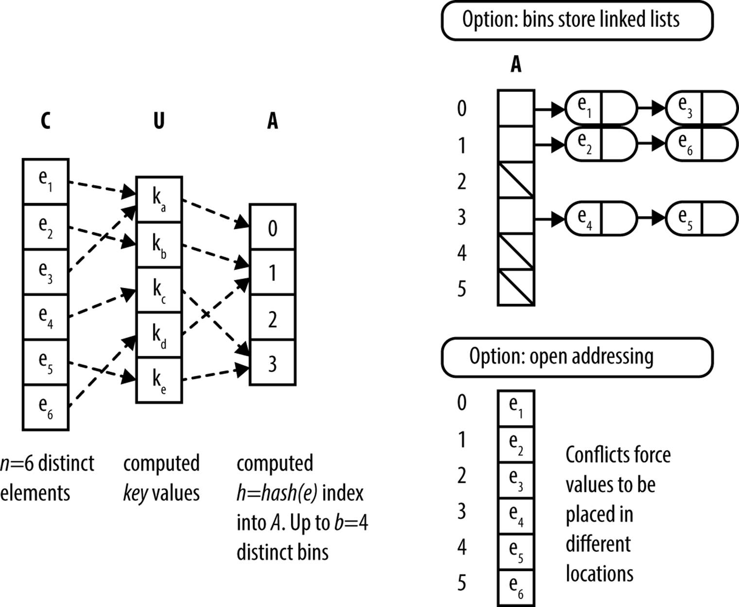
Figure 5-1. General approach to hashing

Input/Output

Unlike Binary Search, the original collection C does not need to be ordered for Hash-Based Search. Indeed, even if the elements in C were ordered in some way, the hashing method that inserts elements into the hash table H does not attempt to replicate this ordering within H.

The input to Hash-Based Search is the computed hash table, H, and the target element t being sought. The algorithm returns true if t exists in the linked list stored by H[h] where h = hash(t). If t does not exist within the linked list stored by H[h], false is returned to indicate t is not present in H (and thus, does not exist in C).

Context

Assume you had an array of 213,557 sorted English words (such as found in the code repository for this book). We know from our discussion on Binary Search that we can expect about 18 string comparisons on average to locate a word in this array (since log (213557) = 17.70). With Hash-Based Search the number of string comparisons is based on the length of the linked lists rather than the size of the collection.

We first need to define the hash function. One goal is to produce as many different values as possible, but not all values need to be unique. Hashing has been studied for decades, and numerous papers describe effective hash functions, but they can be used for much more than searching. For example, special hash functions are essential for cryptography. For searching, a hash function should have good distribution and should be quick to compute with respect to machine cycles.

HASH-BASED SEARCH SUMMARY

Best, Average: O(1) Worst: O(n)

loadTable (size, C)

H = new array of given size

foreach e in C do

h = hash(e)

if H[h] is empty then

H[h] = new Linked List

add e to H[h]

return A

end

search (H, t)

h = hash(t)

list = H[h]

if list is empty then

return false

if list contains t then

return true

return false

end

Create linked lists when e is inserted into empty bin.

Use Sequential Search on small lists.

A popular technique is to produce a value based on each character from the original string:

hashCode(s) = s[0]*31⁽len–1⁾ + s[1]*31⁽len–2⁾ + ... + s[len – 1]

where s[i] is the i^th character (as an ASCII value between 0 and 255) and len is the length of the string s. Computing this function is simple, as shown in the Java code in Example 5-5 (adapted from the Open JDK source code), where chars is the array of characters that defines a string. By our definition, the hashCode() method for the java.lang.String class is not yet a hash function because its computed value is not guaranteed to be in the range [0, b).

Example 5-5. Sample Java hashCode

public int hashCode() {

int h = hash;

if (h == 0) {

for (int i = 0; i < chars.length; i++) {

h = 31*h + chars[i];

}

hash = h;

}

return h;

}

For efficiency, this hashCode method caches the value of the computed hash to avoid recomputation (i.e., it computes the value only if hash is 0). Observe that this function returns very large integers and sometimes negative values because the int type in Java can store only 32 bits of information. To compute the integer bin for a given element, define hash(s) as:

hash(s) = abs(hashCode(s)) % b

where abs is the absolute value function and % is the modulo operator that returns the remainder when dividing by b. Doing so ensures the computed integer is in the range [0, b).

Choosing the hashing function is just the first decision to make when implementing Hash-Based Search. Storage space poses another design issue. The primary storage, H, must be large enough to reduce the size of the linked lists storing the elements in each bin. You might think that Hcould contain b = n bins, where the hash function is a one-to-one mapping from the set of strings in the collection onto the integers [0, n), but this is not easy to accomplish! Instead, we try to define a hash table that will contain as few empty bins as possible. If our hash function distributes the keys evenly, we can achieve reasonable success by selecting an array size approximately as large as the collection.

The size of H is typically chosen to be a prime number to ensure that using the % modulo operator efficiently distributes the computed bin numbers. A good choice in practice is 2^k − 1, even though this value isn’t always prime.

The elements stored in the hash table have a direct effect on memory. Since each bin stores elements in a linked list, the elements of the list are pointers to objects on the heap. Each list has overhead storage that contains pointers to the first and last elements of the list and, if you use theLinkedList class from the Java JDK, a significant amount of additional fields. We could write a much simpler linked list class that provides only the necessary capabilities, but this certainly adds additional cost to the implementation of Hash-Based Search.

The advanced reader should, at this point, question the use of a basic hash function and hash table for this problem. When the word list is fixed and not likely to change, we can do better by creating a perfect hash function. A perfect hash function is one that guarantees no collisions for a specific set of keys; this option is discussed in “Variations”. Let’s first try to solve the problem without one.

For our first try at this problem, we choose a primary hash table H that will hold b = 2¹⁸ − 1 = 262,143 elements. Our word list contains 213,557 words. If our hash function perfectly distributes the strings, there will be no collisions and only about 40,000 open bins. This, however, is not the case. Table 5-4 shows the distribution of the hash values for the Java String class on our word list with a table of 262,143 bins. Recall that hash(s) = abs(hashCode(s))%b. As you can see, no bin contains more than seven strings; for nonempty bins, the average number of strings per bin is approximately 1.46. Each row shows the number of bins used and how many words hash to those bins. Almost half of the table bins (116,186) have no strings that hash to them. So this hashing function wastes about 500KB of memory (assuming the size of a pointer is four bytes). You may be surprised that this is really a good hashing function and that finding one with better distribution will require a more complex scheme.

For the record, there were only five pairs of strings with identical hashCode values (e.g., both “hypoplankton” and “unheavenly” have a computed hashCode value of 427,589,249)!

If you use the LinkedList class, each nonempty element of H will require 12 bytes of memory, assuming the size of a pointer is four bytes. Each string element is incorporated into a ListElement that requires an additional 12 bytes. For the previous example of 213,557 words, we require 5,005,488 bytes of memory beyond the actual string storage. The breakdown of this memory usage is:

§ Size of the primary table: 1,048,572 bytes

§ Size of 116,186 linked lists: 1,394,232 bytes

§ Size of 213,557 list elements: 2,562,684 bytes

Storing the strings also has an overhead when using the JDK String class. Each string has 12 bytes of overhead. We can therefore add 213,557*12 = 2,562,684 additional bytes to our overhead. So the algorithm chosen in the example requires 7,568,172 bytes of memory. The actual number of characters in the strings in the word list we used in the example is only 2,099,075, so it requires approximately 3.6 times the space required for the characters in the strings.

Most of this overhead is the price of using the classes in the JDK. The engineering trade-off must weigh the simplicity and reuse of the classes compared to a more complex implementation that reduces the memory usage. When memory is at a premium, you can use one of several variations discussed later to optimize memory usage. If, however, you have available memory, a reasonable hash function that does not produce too many collisions, and a ready-to-use linked list implementation, the JDK solution is usually acceptable.

The major force affecting the implementation is whether the collection is static or dynamic. In our example, the word list is fixed and known in advance. If, however, we have a dynamic collection that requires many additions and deletions of elements, we must choose a data structure for the hash table that optimizes these operations. Our collision handling in the example works quite well because inserting an item into a linked list can be done in constant time, and deleting an item is proportional to the length of the list. If the hash function distributes the elements evenly, the individual lists are relatively short.

Solution

In addition to the hash function, the solution for Hash-Based Search contains two parts. The first is to create the hash table. The code in Example 5-6 shows how to use linked lists to hold the elements that hash into a specific table element. The input elements from collection C are retrieved using an Iterator.

Example 5-6. Loading the hash table

public void load (Iterator<V> it) {

table = (LinkedList<V>[]) new LinkedList[tableSize];

// Pull each value from the iterator and find desired bin h.

// Add to existing list or create new one into which value is added.

while (it.hasNext()) {

V v = it.next();

int h = hashMethod.hash (v);

if (table[h] == null) {

table[h] = new LinkedList<V>();

}

table[h].add(v);

count++;

}

}

Note that listTable is composed of tableSize bins, each of which is of type LinkedList<V> to store the elements.

Searching the table for elements now becomes trivial. The code in Example 5-7 does the job. Once the hash function returns an index into the hash table, we look to see whether the table bin is empty. If it’s empty, we return false, indicating the searched-for string is not in the collection. Otherwise, we search the linked list for that bin to determine the presence or absence of the searched-for string.

Example 5-7. Searching for an element

public boolean search (V v) {

int h = hashMethod.hash (v);

LinkedList<V> list = (LinkedList<V>) listTable[h];

if (list == null) { return false; }

return list.contains (v);

}

int hash(V v) {

int h = v.hashCode();

if (h < 0) { h = 0 - h; }

return h % tableSize;

}

Note that the hash function ensures the hash index is in the range [0, tableSize). With the hashCode function for the String class, the hash function must account for the possibility that the integer arithmetic in hashCode has overflowed and returned a negative number. This is necessary because the modulo operator (%) returns a negative number if given a negative value (i.e., the Java expression −5%3 is equal to the value −2). For example, using the JDK hashCode method for String objects, the string “aaaaaa” returns the value −1,425,372,064.

Analysis

As long as the hash function distributes the elements in the collection fairly evenly, Hash-Based Search has excellent performance. The average time required to search for an element is constant, or O(1). The search consists of a single look-up in H followed by a linear search through a short list of collisions. The components to searching for an element in a hash table are:

§ Computing the hash value

§ Accessing the item in the table indexed by the hash value

§ Finding the specified item in the presence of collisions

All Hash-Based Search algorithms share the first two components; different behaviors stem from variations in collision handling.

The cost of computing the hash value must be bounded by a fixed, constant upper bound. In our word list example, computing the hash value was proportional to the length of the string. If T_k is the time it takes to compute the hash value for the longest string, it will require ≤ T_k to compute any hash value. Computing the hash value is therefore considered a constant time operation.

The second part of the algorithm also performs in constant time. If the table is stored on secondary storage, there may be a variation that depends on the position of the element and the time required to position the device, but this has a constant upper bound.

If we can show that the third part of the computation also has a constant upper bound, it will prove the overall time performance of Hash-Based Search is constant. For a hash table, define the load factor α to be the average number of elements in a linked list for some bin H[h]. More precisely, α = n/b, where b is the number of bins in the hash table and n is the number of elements stored in the hash table. Table 5-5 shows the actual load factor in the hash tables we create as b increases. Note how the maximum length of the element linked lists drops while the number of bins containing a unique element rapidly increases once b is sufficiently large. In the final row, 81% of the elements are hashed to a unique bin and the average number of elements in a bin becomes just a single digit. Regardless of the initial number of elements, you can choose a sufficiently large b value to ensure there will be a small, fixed number of elements (on average) in every bin. This means that searching for an element in a hash table is no longer dependent on the number of elements in the hash table, but rather is a fixed cost, producing amortized O(1) performance.

Table 5-6 compares the performance of the code from Example 5-7 with the JDK class java.util.Hashtable on hash tables of different sizes. For the tests labeled p = 1.0, each of the 213,557 words is used as the target item to ensure the word exists in the hash table. For the tests labeledp = 0.0, each of these words has its last character replaced with a “*” to ensure the word does not exist in the hash table. Also note that we keep the size of the search words for these two cases the same to ensure the cost for computing the hash is identical.

We ran each test 100 times and discarded the best- and worst-performing trials. The average of the remaining 98 trials is shown in Table 5-6. To help understand these results, the statistics on the hash tables we created are shown in Table 5-5.

As the load factor goes down, the average length of each element-linked list also goes down, leading to improved performance. Indeed, by the time b = 1,045,875 no linked list contains more than five elements. Because a hash table can typically grow large enough to ensure all linked lists of elements are small, its search performance is considered to be O(1). However, this is contingent (as always) on having sufficient memory and a suitable hash function to disperse the elements throughout the bins of the hash table.

The performance of the existing java.util.Hashtable class outperforms our example code, but the savings are reduced as the size of the hash table grows. The reason is that java.util.Hashtable contains optimized list classes that efficiently manage the element chains. In addition,java.util.Hashtable automatically “rehashes” the entire hash table when the load factor is too high; the rehash strategy is discussed in “Variations”. The implementation increases the cost of building the hash table, but improves search performance. If we prevent the “rehash” capability, search performance in java.util.Hashtable is nearly the same as our implementation.

Table 5-7 shows the number of times rehash is invoked when building the java.util.Hashtable hash table and the total time (in milliseconds) required to build the hash table. We constructed the hash tables from the word list described earlier; after running 100 trials, the best- and worst-performing timings were discarded and the table contains the average of the remaining 98 trials. The java.util.Hashtable class performs extra computation while the hash table is being constructed to improve the performance of searches (a common trade-off). Columns 3 and 5 ofTable 5-7 show a noticeable cost penalty when a rehash occurs. Also note that in the last two rows, the hash tables do not rehash themselves, so the results in columns 3, 5, and 7 are nearly identical. Rehashing while building the hash table improves the overall performance by reducing the average length of the element chains.

Variations

One popular variation of Hash-Based Search modifies the handling of collisions by restricting each bin to contain a single element. Instead of creating a linked list to hold all elements that hash to some bin in the hash table, it uses the open addressing technique to store colliding items in some other empty bin in the hash table H. This approach is shown in Figure 5-2. With open addressing, the hash table reduces storage overhead by eliminating all linked lists.

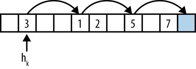
Figure 5-2. Open addressing

To insert an element using open addressing, compute the desired bin h_k = hash(e) that should contain e. If H[h_k] is empty, assign H[h_k] = e just as in the standard algorithm. Otherwise probe through H using a probing strategy and place e in the first discovered empty bin:

Linear probing

Repeatedly search other bins h_k = (h_k + c*i) % b where c is an integer offset and i is the number of successive probes into H; often, c = 1. Clusters of elements may appear in H using this strategy.

Quadratic probing

Repeatedly search other bins h_k = (h_k + c₁*i + c₂*i²) % b where c₁ and c₂ are constants. This approach tends to break up clusters of elements. Useful values in practice are c₁ = c₂ = 1/2.

Double hashing

Like linear probing except that c is not a constant but is determined by a second hash function; this extra computation is intended to reduce the likelihood of clustering.

In all cases, if no empty bin is found after b probe attempts, the insert request must fail.

Figure 5-2 shows a sample hash table with b = 11 bins using linear probing with c = 3. The load factor for the hash table is α = 0.45 because it contains five elements. This figure shows the behavior when attempting to add element e, which hashes to h_k = 1. The bin H[1] is already occupied (by the value 3) so it proceeds to probe other potential bins. After i = 3 iterations it finds an empty bin and inserts e into H[10].

Assuming we only search through b potential bins, the worst-case performance of insert is O(b) but with a low-enough load factor and no clustering, it should require only a fixed number of probes. Figure 5-3 shows the expected number of probes for a search; see (Knuth, 1997) for details.

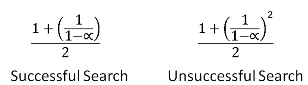
Figure 5-3. The expected number of probes for a search

It is a problem to remove elements from a hash table that uses open addressing. Let’s assume in Figure 5-2 that the values 3, 1, and 5 all hash to h_k = 1 and that they were inserted into the hash table in this order. Searching for the value 5 will succeed because you will make three probes of the hash table and ultimately locate it in position H[7]. If you deleted value 1 from the hash table and cleared bin H[4] you would no longer be able to locate value 5 because the search probes stop at the first empty bin located. To support deletions with open addressing you would need to mark a bin as deleted and adjust the search function accordingly.

The code for open addressing is shown in Example 5-8. The class assumes the user will provide a hash function that produces a valid index in the range [0, b) and a probe function for open addressing; plausible alternatives are provided by default using Python’s built-in hash method. This implementation allows elements to be deleted and it stores a deleted list to ensure the open addressing chains do not break. The following implementation follows set semantics for a collection, and only allows for unique membership in the hash table.

Example 5-8. Python implementation of open addressing hash table

class Hashtable:

def __init__(self, b=1009, hashFunction=None, probeFunction=None):

"""Initialize a hash table with b bins, given hash function, and

probe function."""

self.b = b

self.bins = [None] * b

self.deleted = [False] * b

if hashFunction:

self.hashFunction = hashFunction

else:

self.hashFunction = lambda value, size: hash(value) % size

if probeFunction:

self.probeFunction = probeFunction

else:

self.probeFunction = lambda hk, size, i : (hk + 37) % size

def add (self, value):

"""

Add element into hashtable returning -self.b on failure after

self.b tries. Returns number of probes on success.

Add into bins that have been marked for deletion and properly

deal with formerly deleted entries.

"""

hk = self.hashFunction (value, self.b)

ctr = 1

while ctr <= self.b:

if self.bins[hk] isNone orself.deleted[hk]:

self.bins[hk] = value

self.deleted[hk] = False

return ctr

# already present? Leave now

if self.bins[hk] == value and notself.deleted[hk]:

return ctr

hk = self.probeFunction (hk, self.b, ctr)

ctr += 1

return -self.b

The code in Example 5-8 shows how open addressing adds elements into empty bins or bins marked as deleted. It maintains a counter that ensures the worst-case performance is O(b). The caller can determine that add was successful if the function returns a positive number; ifprobeFunction is unable to locate an empty bin in b tries, then a negative number is returned. The delete code in Example 5-9 is nearly identical to the code to check whether the hash table contains a value; specifically, the contains method (not reproduced here) omits the code that marks self.deleted[hk] = True. Observe how this code uses the probeFunction to identify the next bin to investigate.

Example 5-9. Open addressing delete method

def delete (self, value):

"""Delete value from hash table without breaking existing chains."""

hk = self.hashFunction (value, self.b)

ctr = 1

while ctr <= self.b:

if self.bins[hk] isNone:

return -ctr

if self.bins[hk] == value and notself.deleted[hk]:

self.deleted[hk] = True

return ctr

hk = self.probeFunction (hk, self.b, ctr)

ctr += 1

return -self.b

Let’s review the performance of open addressing by considering how many probes it takes to locate an element in the hash table. Figure 5-4 shows the results for both successful and unsuccessful searches, using the same list of 213,557 words as before. As the number of bins increases—from 224,234 (or 95.2% full) to 639,757 (or 33.4% full)—you can see how the number of probes decreases dramatically. The top half of this figure shows the average (and worst) number of probes for a successful search while the bottom presents the same information for unsuccessful searches. In brief, open addressing reduces the overall storage used but requires noticeably more probes in the worst case. A second implication is that linear probing leads to more probes due to clustering.

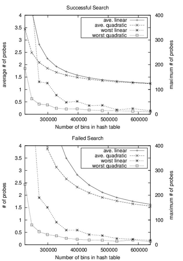
Figure 5-4. Performance of open addressing

Computing the load factor for a hash table describes the expected performance for searching and insertions. If the load factor is too high, the number of probes to locate an item becomes excessive, whether in a bucket’s linked list or a chain of bins in open addressing. A hash table can increase the number of bins and reconstitute itself using a process known as “rehashing,” an infrequent operation that reduces the load factor, although it is a costly O(n) operation. The typical way to do this is to double the number of bins and add one (because hash tables usually contain an odd number of bins). Once more bins are available, all existing elements in the hash table are rehashed and inserted in the new structure. This expensive operation reduces the overall cost of future searches, but it must be run infrequently; otherwise, you will not observe the amortized O(1) performance of the hash tables.

A hash table should rehash its contents when it detects uneven distribution of elements. This can be done by setting a threshold value that will trigger a rehash when the load factor for the hash table exceeds that value. The default threshold load factor for the java.util.Hashtable class is 0.75; if the threshold is large enough, the hash table will never rehash.

These examples use a fixed set of strings for the hash table. When confronted with this special case, it is possible to achieve optimal performance by using perfect hashing, which uses two hash functions. A standard hash() function indexes into the primary table, H. Each bin, H[i], then points to a smaller secondary hash table, S_i, that has an associated hash function hash_i. If there are k keys that hash to bin H[i], S_i will contain k² bins. This seems like a lot of wasted memory, but judicious choice of the initial hash function can reduce this to an amount similar to previous variations. The selection of appropriate hash functions guarantees there are no collisions in the secondary tables. This means we have an algorithm with constant O(1) performance in every case.

Details on the analysis of perfect hashing can be found in (Cormen et al., 2009). Doug Schmidt (1990) has written an excellent paper on perfect hashing generation and there are freely available perfect hash function generators in various programming languages. GPERF for C and C++ can be downloaded from http://www.gnu.org/software/gperf, and JPERF for Java can be downloaded from http://www.anarres.org/projects/jperf.

Bloom Filter

Hash-Based Search stores the full set of values from a collection C in a hash table H, whether in linked lists or using open addressing. In both cases, as more elements are added to the hash table, the time to locate an element increases unless you also increase the amount of storage (in this case, the number of bins). Indeed, this is the behavior expected of all other algorithms in this chapter and we only seek a reasonable trade-off in the amount of space required to reduce the number of comparisons when looking for an element in the collection.

A Bloom Filter provides an alternative bit array structure B that ensures constant performance when adding elements from C into B or checking whether an element has not been added to B; amazingly, this behavior is independent of the number of items already added to B. There is a catch, however; with a Bloom Filter, checking whether an element is in B might return a false positive even though the element does not exist in C. The Bloom Filter can accurately determine when an element has not been added to B, so it never returns a false negative.

In Figure 5-5, two values, u and v, have been inserted into the bit array, B. The table at the top of the figure shows the bit positions computed by k = 3 hash functions. As you can see, the Bloom Filter can quickly demonstrate that a third value w has not been inserted into B, because one of itsk computed bit values is zero (bit 6 in this case). However for value x, it returns a false positive since that value was not inserted, yet all k of its computed bit values are one.

BLOOM FILTER SUMMARY

Best, Average, Worst: O(k)

create(m)

return bit array of m bits

end

add (bits,value)

foreach hashFunction hf

setbit = 1 << hf(value)

bits |= setbit

end

search (bits,value)

foreach hashFunction hf

checkbit = 1 << hf(value)

if checkbit | bits = 0 then

return false

return true

end

Storage is fixed in advance to m bits.

There are k hash functions that compute (potentially) different bit positions.

The << left shift operator efficiently computes 2^hf(value).

Set k bits when inserting value.

When searching for a value, if a computed bit is zero then that value can’t be present.

It may yet be the case that all bits are set but value was never added: false positive.

Input/Output

A Bloom Filter processes values much like Hash-Based Search. The algorithm starts with a bit array of m bits, all set to zero. There are k hash functions that compute (potentially different) bit positions within this bit array when values are inserted.

The Bloom Filter returns false when it can demonstrate that a target element t has not yet been inserted into the bit array, and by extension does not exist in the collection C. The algorithm may return true as a false positive if the target element t was not inserted into the bit array.

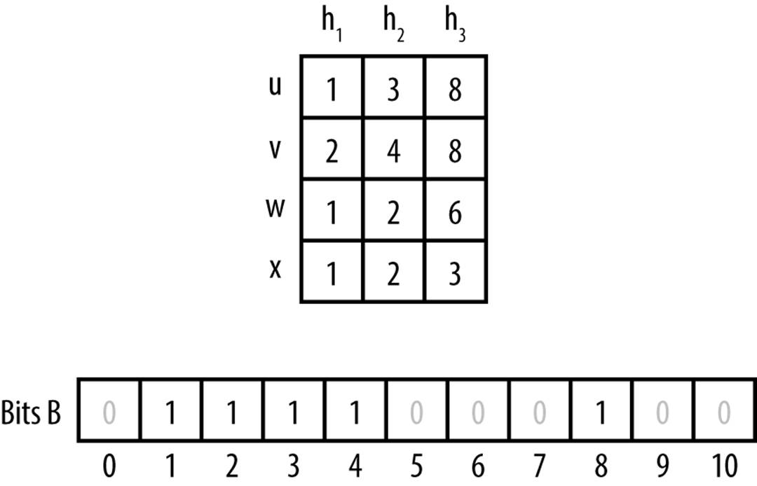
Figure 5-5. Bloom Filter example

Context

A Bloom Filter demonstrates efficient memory usage but it is only useful when false positives can be tolerated. Use a Bloom Filter to reduce the number of expensive searches by filtering out those that are guaranteed to fail—for example, use a Bloom Filter to confirm whether to conduct an expensive search over disk-based storage.

Solution

A Bloom Filter needs m bits of storage. The implementation in Example 5-10 uses Python’s ability to work with arbitrarily large “bignum” values.

Example 5-10. Python Bloom Filter

class bloomFilter:

def __init__(self, size = 1000, hashFunctions=None):

"""

Construct a bloom filter with size bits (default: 1000) and the

associated hash functions.

"""

self.bits = 0

self.size = size

if hashFunctions isNone:

self.k = 1

self.hashFunctions = [lambda e, size : hash(e) % size]

else:

self.k = len(hashFunctions)

self.hashFunctions = hashFunctions

def add (self, value):

"""Insert value into the bloom filter."""

for hf inself.hashFunctions:

self.bits |= 1 << hf (value, self.size)

def __contains__ (self, value):

"""

Determine whether value is present. A false positive might be

returned even if the element is not present. However, a false

negative will never be returned (i.e., if the element is

present, then it will return True).

"""

for hf inself.hashFunctions:

if self.bits & 1 << hf (value, self.size) == 0:

return False

# might be present

return True

This implementation assumes the existence of k hash functions, each of which takes the value to be inserted and the size of the bit array. Whenever a value is added, k bits are set in the bit array, based on the individual bit positions computed by the hash functions. This code uses the bitwise shift operator << to shift a 1 to the appropriate bit position, and the bitwise or operator (|) to set that bit value. To determine whether a value has been added, check the same k bits from these hash functions using the bitwise and operator (&); if any bit position is set to 0, you know the value could not have been added, so it returns False. However, if these k bit positions are all set to 1, you can only state that the value “might” have been added.

Analysis

The total storage required for a Bloom Filter is fixed to be m bits, and this won’t increase regardless of the number of values stored. Additionally, the algorithm only requires a fixed number of k probes, so each insertion and search can be processed in O(k) time, which is considered constant. It is for these reasons that we present this algorithm as a counterpoint to the other algorithms in this chapter. It is challenging to design effective hash functions to truly distribute the computed bits for the values to be inserted into the bit array. While the size of the bit array is constant, it may need to be quite large to reduce the false positive rate. Finally, there is no ability to remove an element from the filter since that would potentially disrupt the processing of other values.

The only reason to use a Bloom Filter is that it has a predicable false positive rate, p^k, assuming the k hash functions are uniformly random (Bloom, 1970). A reasonably accurate computation for p^k is:

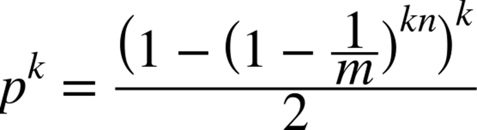
where n is the number of values already added (Bose et al., 2008). We empirically computed the false positive rate as follows:

1. Randomly remove 2,135 words from the list of 213,557 words (1% of the full list) and insert the remaining 211,422 words into a Bloom Filter.

2. Count the false positives when searching for the missing 2,135 words.

3. Count the false positives when searching for 2,135 random strings (of between 2 and 10 lowercase letters).

We ran trials for m with values of 100,000 to 2,000,000 (steps of 10,000). We used k = 3 hash functions. The results are found in Figure 5-6.

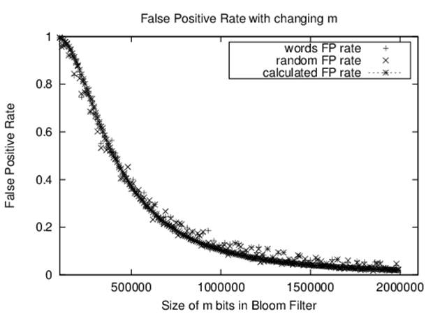
Figure 5-6. Bloom Filter example

If you know in advance that you want your false positive rate to be smaller than some small value, you need to set k and m after estimating the number of elements n to insert. The literature suggests trying to ensure 1 – (1 – 1/m)kn is close to 1/2. For example, to ensure a false positive rate of smaller than 10% for the word list, be sure to set m to at least 1,120,000 or a total of 131,250 bytes.

Binary Search Tree

Binary searching on an array in memory is efficient, as we have already seen. However, using ordered arrays becomes drastically less effective when the underlying collection changes frequently. With a dynamic collection, we must adopt a different data structure to maintain acceptable search performance. Hash-Based Search can handle dynamic collections, but we might select a hash table size that is much too small for effective resource usage; we often have no a priori knowledge of the number of elements to store so it is hard to select the proper size of the hash table. Hash tables do not allow you to iterate over their elements in sorted order.

An alternate strategy is to use a search tree to store dynamic sets. Search trees perform well both in memory and in secondary storage and make it possible to return ordered ranges of elements together, something hash tables are unable to accomplish. The most common type of search tree is the binary search tree (BST), which is composed of nodes as shown in Figure 5-7. Each node contains a single value in the collection and stores references to potentially two child nodes, left and right.

Use a binary search tree when:

§ You must traverse the data in ascending (or descending) order

§ The data set size is unknown, and the implementation must be able to handle any possible size that will fit in memory

§ The data set is highly dynamic, and there will be many insertions and deletions during the collection’s lifetime

Input/Output

The input and output to algorithms using search trees is the same as for Binary Search. Each element e from a collection C to be stored in the binary search tree needs to have one or more properties that can be used as a key k; these keys determine the universe U and must be fully ordered. That is, given two key values k_i and k_j, either k_i equals k_j, k_i > k_j, or k_i < k_j.

When the values in the collections are primitive types (such as strings or integers), the values themselves can be the key values. Otherwise, they are references to the structures that contain the values.

Context

A BST is a nonempty collection of nodes containing ordered values known as keys. The top root node is the ancestor of all other nodes in the BST. Each node n may potentially refer to two binary nodes, n_left and n_right, each the root of BSTs left and right. A BST ensures the binary search tree property, namely, that if k is the key for node n, then all keys in left ≤ k and all the keys in right ≥ k. If both n_left and n_right are null, then n is a leaf node. Figure 5-7 shows a small example of a BST where each node contains an integer value. The root contains the value 7 and there are four leaf nodes containing values 1, 6, 10, and 17. An interior node, such as 5, has both a parent node and some children nodes. You can see that finding a key in the tree in Figure 5-7 requires examining at most four nodes, starting with the root.

A BST might not be balanced; as elements are added, some branches may end up relatively short while others become longer. This produces suboptimal search times on the longer branches. In the worst case, the structure of a BST might degenerate and take on the basic properties of a list. Consider the same values for Figure 5-7 arranged as shown in Figure 5-8. Although the structure fits the strict definition of a BST, the structure is effectively a linked list because the right subtree of each node is empty.

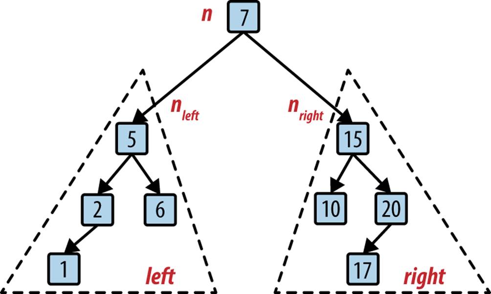
Figure 5-7. A simple binary search tree

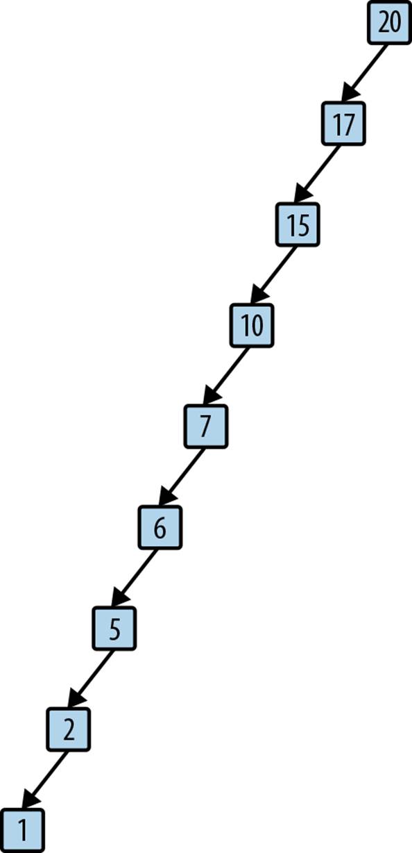
Figure 5-8. A degenerate binary search tree

You must balance the tree to avoid a skewed tree that has a few branches that are much longer than the other branches. We present a full solution for a balanced AVL tree supporting insertion and deletion of values.

Solution

The initial Python structure is shown in Example 5-11 together with the add methods necessary to add values to the BST. The methods are recursive, going down a branch from the root until an empty place for the new node is found at the right position.

Example 5-11. Python Binary Search Tree class definition

class BinaryNode:

def __init__(self, value = None):

"""Create binary node."""

self.value = value

self.left = None

self.right = None

def add (self, val):

"""Adds a new node to BST with given value."""

if val <= self.value:

if self.left:

self.left.add (val)

else:

self.left = BinaryNode(val)

else:

if self.right:

self.right.add(val)

else:

self.right = BinaryNode(val)

class BinaryTree:

def __init__(self):

"""Create empty BST."""

self.root = None

def add (self, value):

"""Insert value into proper location in BST."""

if self.root isNone:

self.root = BinaryNode(value)

else:

self.root.add (value)

Adding a value to an empty BST creates the root node; thereafter, the inserted values are placed into new BinaryNode objects at the appropriate place in the BST. There can be two or more nodes in the BST with the same value, but if you want to restrict the tree to conform to set-based semantics (such as defined in the Java Collections Framework) you can modify the code to prevent the insertion of duplicate keys. For now, assume that duplicate keys may exist in the BST.

With this structure in place, the nonrecursive contains(value) method in the BinaryTree class, shown in Example 5-12, searches for a target value within the BST. Rather than perform a recursive function call, this simply traverses left or right pointers until it finds the target or determines that the target does not exist in the BST.

Example 5-12. BinaryTree contains method

def __contains__ (self, target):

"""Check whether BST contains target value."""

node = self.root

while node:

if target < node.value:

node = node.left

ielif target > node.value:

node = node.right

else:

node = node.right

return true

The efficiency of this implementation depends on whether the BST is balanced. For a balanced tree, the size of the collection being searched is cut in half with each pass through the while loop, resulting in O(log n) behavior. However, for a degenerate binary tree such as shown in Figure 5-8, the performance is O(n). To preserve optimal performance, you need to balance a BST after each addition (and deletion).

AVL trees (named after their inventors, Adelson-Velskii and Landis) were the first self-balancing BST, invented in 1962. Let’s define the concept of an AVL node’s height. The height of a leaf node is 0, because it has no children. The height of a nonleaf node is 1 greater than the maximum of the height values of its two children nodes. For consistency, the height of a nonexistent child node is –1.

An AVL tree guarantees the AVL property at every node, namely, that the height difference for any node is –1, 0, or 1. The height difference is defined as height(left) – height(right)—that is, the height of the left subtree minus the height of the right subtree. An AVL tree must enforce this property whenever a value is inserted or removed from the tree. Doing so requires two helper methods: computeHeight to compute the height of a node and heightDifference to compute the height difference. Each node in the AVL tree stores its height value, which increases the overall storage requirements.

Figure 5-9 demonstrates what happens when you insert the values 50, 30, and 10 into a BST in that order. As shown, the resulting tree no longer satisfies the AVL property because the height of the root’s left subtree is 1 while the height of its non-existing right subtree is –1, resulting in a height difference of 2. Imagine “grabbing” the 30 node in the original tree and rotating the tree to the right (or clockwise), and pivoting around the 30 node to make 30 the root, thereby creating a balanced tree (shown in Figure 5-10). In doing so, only the height of the 50 node has changed (dropping from 2 to 0) and the AVL property is restored.

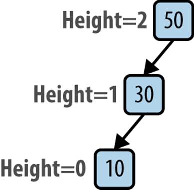
Figure 5-9. Unbalanced AVL tree

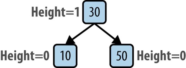
Figure 5-10. Balanced AVL tree

This rotate right operation alters the structure of a subtree within an unbalanced BST; as you can imagine, there is a similar rotate left operation.

What if this tree had other nodes, each of which were balanced and satisfied the AVL property? In Figure 5-11, each of the shaded triangles represents a potential subtree of the original tree; each is labeled by its position, so 30R is the subtree representing the right subtree of node 30. The root is the only node that doesn’t support the AVL property. The various heights in the tree are computed assuming the node 10 has some height k.

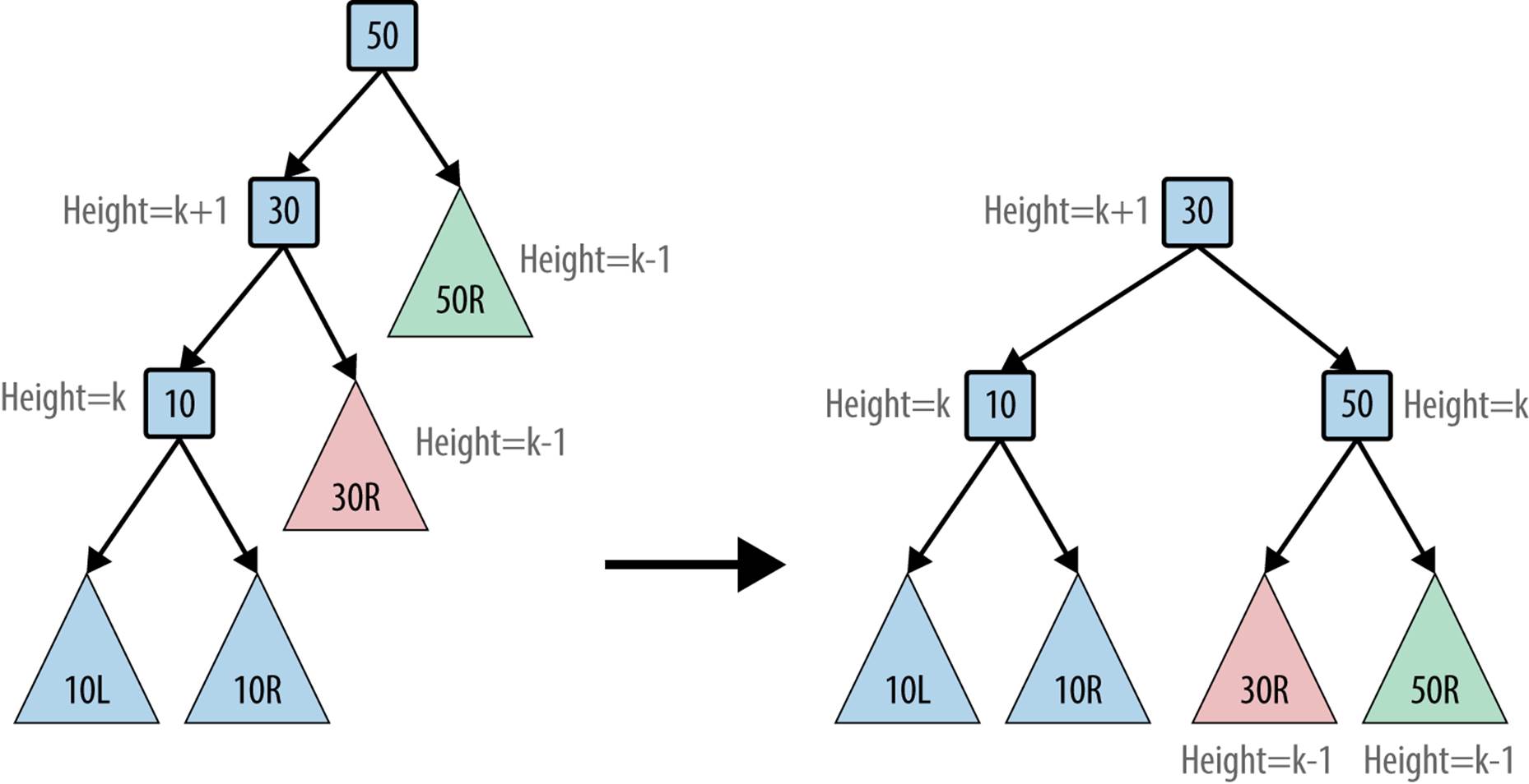
Figure 5-11. Balanced AVL tree with subtrees

The modified BST still guarantees the binary search property. All of the key values in the subtree 30R are greater than or equal to 30. The other subtrees have not changed positions relative to each other, so they continue to guarantee the binary search property. Finally, the value 30 is smaller than 50, so the new root node is valid.

Consider adding three values to an empty AVL tree; Figure 5-12 shows the four different insert orders that result in an unbalanced tree. In the Left-Left case you perform a rotate right operation to rebalance the tree; similarly, in the Right-Right case you perform a rotate left operation. However, in the Left-Right case, you cannot simply rotate right because the “middle” node, 10, cannot become the root of the tree; its value is smaller than both of the other two values.

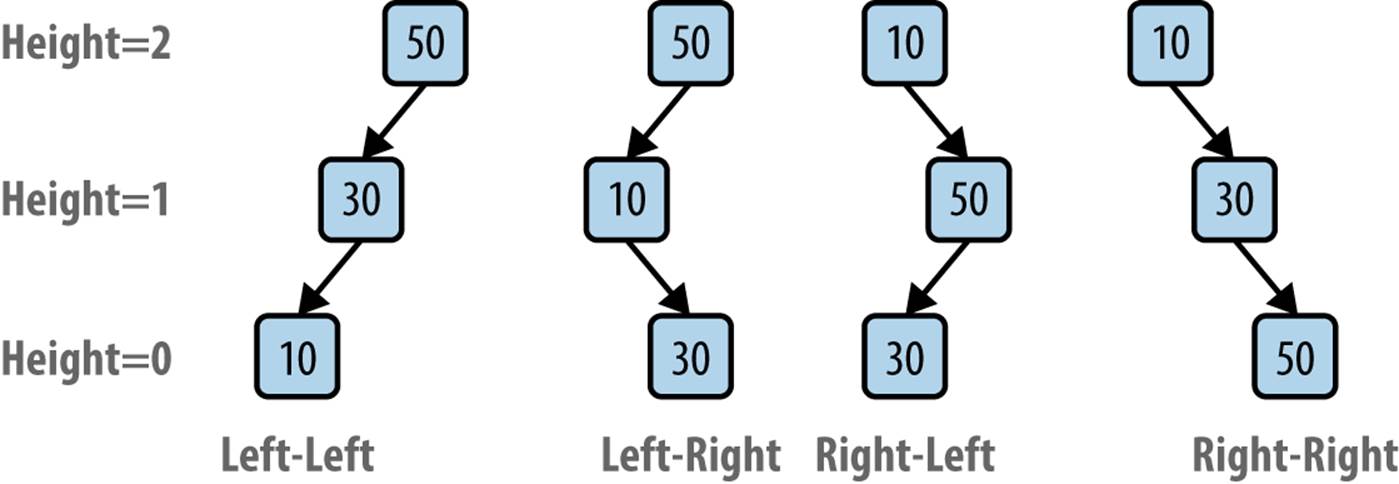
Figure 5-12. Four unbalanced scenarios

Fortunately, you can resolve the issue by first completing a rotate left on the child node 10 to convert the tree into a Left-Left case; then you’ll be able to perform the rotate right step as described earlier. Figure 5-13 demonstrates this situation on a larger tree. After the rotate left operation, the tree is identical to the earlier tree on which the rotate right operation was described. A similar argument explains how to handle the Right-Left case.

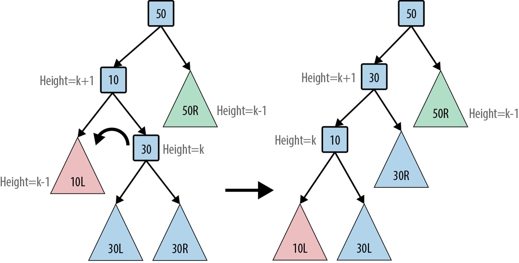
Figure 5-13. Rebalancing the Left-Right scenario

The recursive add operation shown in Example 5-13 has the same structure as Example 5-11 and the difference is that it may need to rebalance the tree once the value is inserted as a newly added leaf node. The BinaryNode add operation adds the new value to the BST rooted at that node and returns a BinaryNode object, which is to become the new root of that BST. This happens because a rotation operation moves a new node to be the root of that BST. Because BSTs are recursive structures, you should realize that the rotation can happen at any point. It is for this reason that the recursive invocation within add has the form self.left = self.addToSubTree(self.left, val). After adding val to the subtree rooted at self.left, that subtree might have rebalanced to have a new node to be its root, and that new node must now become the left child ofself. The final act of add is to compute its height to allow the recursion to propagate back up to the original root of the tree.

Example 5-13. add methods in BinaryTree and BinaryNode

class BinaryTree:

def add (self, value):

"""Insert value into proper location in Binary Tree."""

if self.root isNone:

self.root = BinaryNode(value)

else:

self.root = self.root.add (value)

class BinaryNode:

def __init__(self, value = None):

"""Create binary node."""

self.value = value

self.left = None

self.right = None

self.height = 0

def computeHeight (self):

"""Compute height of node in BST from children."""

height = -1

if self.left:

height = max(height, self.left.height)

if self.right:

height = max(height, self.right.height)

self.height = height + 1

def heightDifference(self):

"""Compute height difference of node's children in BST."""

leftTarget = 0

rightTarget = 0

if self.left:

leftTarget = 1 + self.left.height

if self.right:

rightTarget = 1 + self.right.height

return leftTarget - rightTarget

def add (self, val):

"""Adds a new node to BST with value and rebalance as needed."""

newRoot = self

if val <= self.value:

self.left = self.addToSubTree (self.left, val)

if self.heightDifference() == 2:

if val <= self.left.value:

newRoot = self.rotateRight()

else:

newRoot = self.rotateLeftRight()

else:

self.right = self.addToSubTree (self.right, val)

if self.heightDifference() == -2:

if val > self.right.value:

newRoot = self.rotateLeft()

else:

newRoot = self.rotateRightLeft()

newRoot.computeHeight()

return newRoot

def addToSubTree (self, parent, val):

"""Add val to parent subtree (if exists) and return root in case it

has changed because of rotation."""

if parent isNone:

return BinaryNode(val)

parent = parent.add (val)

return parent

The compact implementation of add shown in Example 5-13 has an elegant left or right as circumstances require, untiladdToSubTree eventually is asked to add val to an empty subtree (i.e., when parent is None). This terminates the recursion and ensures the newly added value is always a leaf node in the BST. Once this action is completed, each subsequent recursive call ends and add determines whether any rotation is needed to maintain the AVL property. These rotations start deep in the tree (i.e., nearest to the leaves) and work their way back to the root. Because the tree is balanced, the number of rotations is bounded by O(log n). Each rotation method has a fixed number of steps to perform; thus the extra cost for maintaining the AVL property is bounded by O(log n). Example 5-14 contains the rotateRight and rotateRightLeft operations.

Example 5-14. rotateRight and rotateRightLeft methods

def rotateRight (self):

"""Perform right rotation around given node."""

newRoot = self.left

grandson = newRoot.right

self.left = grandson

newRoot.right = self

self.computeHeight()

return newRoot

def rotateRightLeft (self):

"""Perform right, then left rotation around given node."""

child = self.right

newRoot = child.left

grand1 = newRoot.left

grand2 = newRoot.right

child.left = grand2

self.right = grand1

newRoot.left = self

newRoot.right = child

child.computeHeight()

self.computeHeight()

return newRoot

For completeness, Example 5-15 lists the rotateLeft and rotateLeftRight methods.

Example 5-15. rotateLeft and rotateLeftRight methods

def rotateLeft (self):

"""Perform left rotation around given node."""

newRoot = self.right

grandson = newRoot.left

self.right = grandson

newRoot.left = self

self.computeHeight()

return newRoot

def rotateLeftRight (self):

"""Perform left, then right rotation around given node."""

child = self.left

newRoot = child.right

grand1 = newRoot.left

grand2 = newRoot.right

child.right = grand1

self.left = grand2

newRoot.left = child

newRoot.right = self

child.computeHeight()

self.computeHeight()

return newRoot

To complete the dynamic behavior of the BST, we need to be able to remove elements efficiently. When removing a value from the BST, it is critical to maintain the binary search tree property. If the target node containing the value to be removed has no left child, you can simply “lift” up its right child node to take its place. Otherwise, find the node with the largest value in the tree rooted at the left child. You can swap that largest value into the target node. Note that the largest value in the left subtree has no right child, so you can easily remove it by moving up its left child, should it have one, as shown in Figure 5-14. Example 5-16 shows the necessary methods.

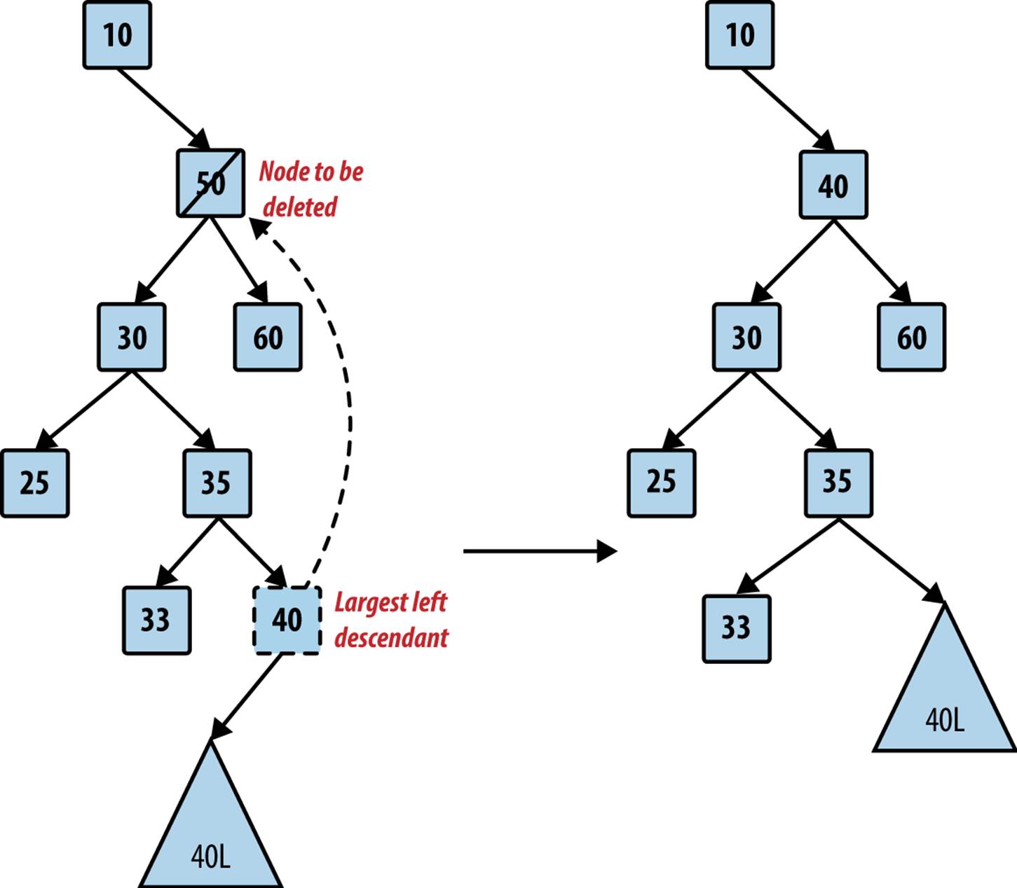
Figure 5-14. Locating largest descendant in left subtree

Example 5-16. BinaryNode remove and removeFromParent methods

def removeFromParent (self, parent, val):

""" Helper method for remove. Ensures proper behavior when

removing node that has children."""

if parent:

return parent.remove (val)

return None

def remove (self, val):

"""

Remove val from Binary Tree. Works in conjunction with

remove method in Binary Tree.

"""

newRoot = self

if val == self.value:

if self.left isNone:

return self.right

child = self.left

while child.right:

child = child.right

childKey = child.value;

self.left = self.removeFromParent (self.left, childKey)

self.value = childKey;

if self.heightDifference() == -2:

if self.right.heightDifference() <= 0:

newRoot = self.rotateLeft()

else:

newRoot = self.rotateRightLeft()

elif val < self.value:

self.left = self.removeFromParent (self.left, val)

if self.heightDifference() == -2:

if self.right.heightDifference() <= 0:

newRoot = self.rotateLeft()

else:

newRoot = self.rotateRightLeft()

else:

self.right = self.removeFromParent (self.right, val)

if self.heightDifference() == 2:

if self.left.heightDifference() >= 0:

newRoot = self.rotateRight()

else:

newRoot = self.rotateLeftRight()

newRoot.computeHeight()

return newRoot

The remove code has a structure similar to add. Once the recursive call locates the target node that contains the value to be removed, it checks to see whether there is a larger descendant in the left subtree to be swapped. As each recursive call returns, observe how it checks whether any rotation is needed. Because the depth of the tree is bounded by O(log n), and each rotation method executes a constant time, the total execution time for remove is bounded by O(log n).

The final logic we expect in a BST is the ability to iterate over its contents in sorted order; this capability is simply not possible with hash tables. Example 5-17 contains the necessary changes to BinaryTree and BinaryNode.

Example 5-17. Support for in-order traversal

class BinaryTree:

def __iter__(self):

"""In order traversal of elements in the tree."""

if self.root:

return self.root.inorder()

class BinaryNode:

def inorder(self):

"""In order traversal of tree rooted at given node."""

if self.left:

for n inself.left.inorder():

yield n

yield self.value

if self.right:

for n inself.right.inorder():

yield n

With this implementation in place, you can print out the values of a BinaryTree in sorted order. The code fragment in Example 5-18 adds 10 integers (in reverse order) to an empty BinaryTree and prints them out in sorted order:

Example 5-18. Iterating over the values in a BinaryTree

bt = BinaryTree()

for i inrange(10, 0, -1):

bt.add(i)

for v inbt:

print (v)

Analysis

The average-case performance of search in a balanced AVL tree is the same as a Binary Search (i.e., O(log n)). Note that no rotations ever occur during a search.

Self-balancing binary trees require more complicated code to insert and remove than simple binary search trees. If you review the rotation methods, you will see that they each have a fixed number of operations, so these can be treated as behaving in constant time. The height of a balanced AVL will always be on the order of O(log n) because of the rotations; thus there will never be more than O(log n) rotations performed when adding or removing an item. We can then be confident that insertions and deletions can be performed in O(log n) time. The trade-off is usually worth it in terms of runtime performance gains. AVL trees store additional height information with each node, increasing storage requirements.

Variations

One natural extension for a binary tree is an n-way tree, where each node has more than one value, and correspondingly, more than two children. A common version of such trees is called the B-Tree, which performs very well when implementing relational databases. A complete analysis of B-Trees can be found in (Cormen et al., 2009) and there are helpful online B-Tree tutorials with examples.

Another common self-balancing binary tree is the red–black tree. Red–black trees are approximately balanced and guarantee that no branch has a height more than twice that of any other branch in the tree. This relaxed guarantee improves the performance of insert and delete by reducing the number of rotations needed. We provide an implementation in the algs.model.tree.BalancedTree class found in the repository. Further details can be found in (Cormen et al., 2009).

References

Adel’son-Vel’skii, G. M. and E. Landis, “An algorithm for the organization of information,” Soviet Mathematics Doklady, 3: 1259–1263, 1962.

Bloom, B., “Space/time trade-offs in hash coding with allowable errors,” Communications of the ACM, 13(7): 422–426, 1970, http://dx.doi.org/10.1145/362686.362692.

Bose, P., H. Guo, E. Kranakis, A. Maheshwari, P. Morin, J. Morrison, M. Smid, and Y. Tang, “On the false-positive rate of Bloom filters,” Information Processing Letters 108: 210–213, 2008, http://dx.doi.org/10.1016/j.ipl.2008.05.018.

Cormen, T. H., C. Leiserson, R. Rivest, and C. Stein, Introduction to Algorithms. Third Edition. MIT Press, 2009.

Hester, J. H. and D. Hirschberg, “Self-organizing linear search,” ACM Computing Surveys, 17(3): 295–311, 1985, http://dx.doi.org/10.1145/5505.5507.

Knuth, D. E., The Art of Computer Programming, Volume 3: Sorting and Searching. Second Edition. Addison-Wesley, 1998.

Schmidt, D., “GPERF: A Perfect Hash Function Generator,” C++ Report, SIGS, 10(10), 1998, http://www.cs.wustl.edu/~schmidt/PDF/gperf.pdf.