Practical Data Science with R (2014)

Appendix A. Working with R and other tools

In this appendix, we’ll show how you can install tools and start working with R. We’ll demonstrate some example concepts and steps, but you’ll want to follow up with additional reading.

A.1. Installing the tools

The primary tool for working our examples will be R as run inside RStudio. But other tools (databases, version control) are also highly recommended. You may also need access to online documentation or other help to get all of these tools to work in your environment. The distribution sites we list are a good place to start.

RStudio and the database tools we suggest require Java. You can download Java from http://www.oracle.com/technetwork/java/javase/downloads/index.html. You won’t need to enable Java in your web browser (Java enabled in the web browser is currently considered an unacceptable security risk).

A.1.1. Installing R

A precompiled version of R can be downloaded from CRAN (http://cran.r-project.org); we recommend picking up RStudio from http://rstudio.com. CRAN is also the central repository for the most popular R libraries. CRAN serves the central role for R, similar to the role that CPAN serves for Perl and CTAN serves for Tex. Follow the instructions given at CRAN to download and install R, and we suggest you install Git and RStudio before starting to use R.

A.1.2. The R package system

R is a broad and powerful language and analysis workbench in and of itself. But one of its real strengths is the depth of the package system and packages supplied through CRAN. To install a package from CRAN, just type install.packages ('nameofpackage'). To use an installed package, type library(nameofpackage). Any time you type library('nameofpackage')^[1] or require('nameofpackage'), you’re assuming you’re using a built-in package or you’re able to run install.packages ('nameofpackage') if needed. We’ll return to the package system again and again in this book. To see what packages are present in your session, type sessionInfo().

¹ Actually, library('nameofpackage') also works with quotes. The unquoted form works in R because R has the ability to delay argument evaluation (so an undefined nameofpackage doesn’t cause an error) as well as the ability to snoop the names of argument variables (most programming languages rely only on references or values of arguments). Given that a data scientist has to work with many tools and languages throughout the day, we prefer to not rely on features unique to one language unless we really need the feature. But the “official R style” is without the quotes.

Changing your CRAN mirror

You can change your CRAN mirror at any time with the chooseCRANmirror() command. This is handy if the mirror you’re working with is slow.

A.1.3. Installing Git

We advise installing Git version control before we show you how to use R and RStudio. This is because without Git, or a tool like it, you’ll lose important work. Not just lose your work—you’ll lose important client work. A lot of data science work (especially the analysis tasks) involves trying variations and learning things. Sometimes you learn something surprising and need to redo earlier experiments. Version control keeps earlier versions of all of your work, so it’s exactly the right tool to recover code and settings used in earlier experiments. Git is available in precompiled packages from http://git-scm.com.

A.1.4. Installing RStudio

RStudio supplies a text editor (for editing R scripts) and an integrated development environment for R. Before picking up RStudio from http://rstudio.com, you should install both R and Git as we described earlier.

The RStudio product you initially want is called RStudio Desktop and is available precompiled for Windows, Linux, and OS X. RStudio is available in 64-bit and 32-bit versions—which version you want depends on whether your operating system is 32- or 64-bit. Use the 64-bit version if you can.

A.1.5. R resources

A lot of the power of R comes from the deep bench of freely available online resources. In this section, we’ll touch on a few sources of code and documentation.

Installing R views

R has an incredibly deep set of available libraries. Usually, R already has the package you want; it’s just a matter of finding it. A powerful way to find R packages is using views: http://cran.r-project.org/web/views/.

You can also install all of the packages (with help documentation) from a view in a single command (though be warned: this can take an hour to finish). For example, here we’re installing a huge set of time series libraries all at once:

install.packages('ctv')

library('ctv')

install.views('TimeSeries')

Once you’ve done this, you’re ready to try examples and code.

Online R resources

A lot of R help is available online. Some of our favorite resources include these:

· CRAN— The main R site: http://cran.r-project.org

· Stack Overflow R section— A question-and-answer site: http://stackoverflow.com/questions/tagged/r

· Quick-R— A great R resource: http://www.statmethods.net

· LearnR— A translation of all the plots from Lattice: Multivariate Data Visualization with R (Use R!) (by D. Sarker; Springer, 2008) into ggplot2: http://learnr.wordpress.com

· R-bloggers— A high-quality R blog aggregator: http://www.r-bloggers.com

A.2. Starting with R

R implements a dialect of a statistical programming language called S. The original implementation of S evolved into a commercial package called S+. So most of R’s language design decisions are really facts about S. To avoid confusion, we’ll mostly just say R when describing features. You might wonder what sort of command and programming environment S/R is. It’s a pretty powerful one, with a nice command interpreter that we encourage you to type directly into.

Working with R and issuing commands to R is in fact scripting or programming. We assume you have some familiarity with scripting (be it Visual Basic, Bash, Perl, Python, Ruby, and so on) or programming (be it C, C#, C++, Java, Lisp, Scheme, and so on), or are willing to use one of our references to learn. We don’t intend to write long programs in R, but we’ll have to show how to issue R commands. R’s programming, though powerful, is a bit different than many of the popular programming languages, but we feel that with a few pointers, anyone can use R. If you don’t know how to use a command, try using the help() call to get at some documentation.

Throughout this book, we’ll instruct you to run various commands in R. This will almost always mean typing the text or the text following the command prompt > into the RStudio console window, followed by pressing Return. For example, if we tell you to type 1/5, you can type that into the console window, and when you press Enter you’ll see a result such as [1] 0.2. The [1] portion of the result is just R’s way of labeling result rows (and is to be ignored), and the 0.2 is the floating point representation of one-fifth, as requested.

Help

Always try calling help() to learn about commands. For example, help('if') will bring up help in R’s if command.

Let’s try a few commands to help you become familiar with R and its basic data types. R commands can be terminated with a line break or a semicolon (or both), but interactive content isn’t executed until you press Return. The following listing shows a few experiments you should run in your copy of R.

Listing A.1. Trying a few R commands

> 1

[1] 1

> 1/2

[1] 0.5

> 'Joe'

[1] "Joe"

> "Joe"

[1] "Joe"

> "Joe"=='Joe'

[1] TRUE

> c()

NULL

> is.null(c())

[1] TRUE

> is.null(5)

[1] FALSE

> c(1)

[1] 1

> c(1,2)

[1] 1 2

> c("Apple",'Orange')

[1] "Apple" "Orange"

> length(c(1,2))

[1] 2

> vec <- c(1,2)

> vec

[1] 1 2

Multiline commands in R

R is good with multiline commands. To enter a multiline command, just make sure it would be a syntax error to stop parsing where you break a line. For example, to enter 1+2 as two lines, add the line break after the plus sign and not before. To get out of R’s multiline mode, press Escape. A lot of cryptic R errors are caused by either a statement ending earlier than you wanted (a line break that doesn’t force a syntax error on early termination) or not ending where you expect (needing an additional line break or semicolon).

A.2.1. Primary features of R

R commands look like a typical procedural programming language. This is deceptive, as the S language (the language R implements) was actually inspired by functional programming and also has a lot of object-oriented features.

Assignment

R has five common assignment operators: =, <-, ->, <<-, and ->>. Traditionally in R, <- is the preferred assignment operator and = is thought as a late addition and an amateurish alias for it.

The main advantage of the <- notation is that <- always means assignment, whereas = can mean assignment, list slot binding, function argument binding, or case statement, depending on context. One mistake to avoid is accidentally inserting a space in the assignment operator:

> x <- 2

> x < - 3

[1] FALSE

> print(x)

[1] 2

We actually like = assignment better because data scientists tend to work in more than one language at a time and more bugs are caught early with =. But this advice is too heterodox to burden others with (see http://mng.bz/hfug). We try to consistently use <- in this book, but some habits are hard to break.

The = operator is also used to bind values to function arguments (and <- can’t be so used) as shown in the next listing.

Listing A.2. Binding values to function arguments

> divide <- function(numerator,denominator) { numerator/denominator }

> divide(1,2)

[1] 0.5

> divide(2,1)

[1] 2

> divide(denominator=2,numerator=1)

[1] 0.5

divide(denominator<-2,numerator<-1) # yields 2, a wrong answer

[1] 2

The -> operator is just a right-to-left assignment that lets you write things like x -> 5. It’s cute, but not game changing.

The <<- and ->> operators are to be avoided unless you actually need their special abilities. What they do is search through parent calling environments (usually associated with a stack of function calls) to find an unlocked existing definition they can alter; or, finding no previous definition, they create a definition in the global environment. The ability evades one of the important safety points about functions. When a variable is assigned inside a function, this assignment is local to the function. Nobody outside of the function ever sees the effect; the function can safely use variables to store intermediate calculations without clobbering same-named outside variables. The <<- and ->> operators reach outside of this protected scope and allow potentially troublesome side effects. Side effects seem great when you need them (often for error tracking and logging), but on the balance they make code maintenance, debugging, and documentation much harder. In the following listing, we show a good function that doesn’t have a side effect and a bad function that does.

Listing A.3. Demonstrating side effects

> x<-1

> good <- function() { x <- 5}

> good()

> print(x)

[1] 1

> bad <- function() { x <<- 5}

> bad()

> print(x)

[1] 5

Vectorized operations

Many R operations are called vectorized, which means they work on every element of a vector. These operators are convenient and to be preferred over explicit code like for loops. For example, the vectorized logic operators are ==, &, and |. The next listing shows some examples using these operators on R’s logical types TRUE and FALSE (which can also be written as T and F).

Listing A.4. R truth tables for Boolean operators

> c(T,T,F,F) == c(T,F,T,F)

[1] TRUE FALSE FALSE TRUE

> c(T,T,F,F) & c(T,F,T,F)

[1] TRUE FALSE FALSE FALSE

> c(T,T,F,F) | c(T,F,T,F)

[1] TRUE TRUE TRUE FALSE

Never use && or || in R

In many C-descended languages, the preferred logic operators are && and ||. R has such operators, but they’re not vectorized, and there are few situations where you want what they do (so using them is almost always a typo or a bug).

To test if two vectors are a match, we’d use R’s identical() or all.equal() methods.

R also supplies a vectorized sector called ifelse(,,) (the basic R-language if statement isn’t vectorized).

R is an object-oriented language

Every item in R is an object and has a type definition called a class. You can ask for the type of any item using the class() command. For example, class(c(1,2)) is numeric. R in fact has two object-oriented systems. The first one is called S3 and is closest to what a C++ or Java programmer would expect. In the S3 class system, you can have multiple commands with the same name. For example, there may be more than one command called print(). Which print() actually gets called when you type print(x) depends on what type x is at runtime. S3 is a bit of a “poor man’s” object-oriented system, as it doesn’t support the more common method notation c(1,2).print() (instead using print(c(1,2))), and methods are just defined willy-nilly and not strongly associated with object definitions, prototypes, or interfaces. R also has a second object-oriented system called S4, which supports more detailed classes and allows methods to be picked based on the types of more than just the first argument. Unless you’re planning on becoming a professional R programmer (versus a professional R user or data scientist), we advise not getting into the complexities of R’s object-oriented systems. Mostly you just need to know that most R objects define useful common methods like print(), summary(), and class(). We also advise leaning heavily on the help() command. To get class-specific help, you use a notationmethod.class; for example, to get information on the predict() method associated with objects of class glm, you would type help(predict.glm).

R is a functional language

Functions are first-class objects in R. You can define anonymous functions on the fly and store functions in variables. For example, here we’re defining and using a function we call add. In fact, our function has no name (hence it’s called anonymous), and we’re just storing it in a variable named add:

> add <- function(a,b) { a + b}

> add(1,2)

[1] 3

To properly join strings in this example, we’d need to use the paste() function.

R is a generic language

R functions don’t use type signatures (though methods do use them to determine the object class). So all R functions are what we call generic. For example, our addition function is generic in that it has no idea what types its two arguments may be or even if the + operator will work for them. We can feed any arguments into add, but sometimes this produces an error:

> add(1,'fred')

Error in a + b : non-numeric argument to binary operator

R is a dynamic language

R is a dynamic language, which means that only values have types, not variables. You can’t know the type of a variable until you look at what value the variable is actually storing. R has the usual features of a dynamic language, such as on-the-fly variable creation. For example, the line x=5either replaces the value in variable x with a 5 or creates a new variable named x with a value of 5 (depending on whether x had been defined before). Variables are only created during assignment, so a line like x=y is an error if y hasn’t already been defined. You can find all of your variables using the ls() command.

Don’t rely on implicit print()

A command that’s just a variable name often is equivalent to calling print() on the variable. But this is only at the so-called “top level” of the R command interpreter. Inside a sourced script, function, or even a loop body, referring to a variable becomes a no-op instead of print(). This is especially important to know for packages like ggplot2 that override the inbuilt print() command to produce desirable side effects like producing a plot.

R behaves like a call-by-value language

R behaves like what’s known as a call-by-value language. That means, from the programmer’s point of view, each argument of a function behaves as if it were a separate copy of what was passed to the function. Technically, R’s calling semantics are actually a combination of references and what is called lazy evaluation. But until you start directly manipulating function argument references, you see what looks like call-by-value behavior.

Call-by-value is a great choice for analysis software: it makes for fewer side effects and bugs. But most programming languages aren’t call-by-value, so call-by-value semantics often come as a surprise. For example, many professional programmers rely on changes made to values inside a function being visible outside the function. Here’s an example of call-by-value at work.

Listing A.5. Call-by-value effect

> vec <- c(1,2)

> fun <- function(v) { v[[2]]<-5; print(v)}

> fun(vec)

[1] 1 5

> print(vec)

[1] 1 2

R isn’t a disciplined language

R isn’t a disciplined language in that there’s usually more than one way to do something. The good part is this allows R to be broad, and you can often find an operator that does what you want without requiring the user to jump through hoops. The bad part is you may find too many options and not feel confident in picking a best one.

A.2.2. Primary R data types

While the R language and its features are interesting, it’s the R data types that are most responsible for R’s style of analysis. In this section, we’ll discuss the primary data types and how to work with them.

Vectors

R’s most basic data type is the vector, or array. In R, vectors are arrays of same-typed values. They can be built with the c() notation, which converts a comma-separated list of arguments into a vector (see help(c)). For example, c(1,2) is a vector whose first entry is 1 and second entry is2. Try typing print(c(1,2)) into R’s command prompt to see what vectors look like and notice that print(class(1)) returns numeric, which is R’s name for numeric vectors.

Numbers in R

Numbers in R are primarily represented in double-precision floating-point. This differs from some programming languages, such as C and Java, that default to integers. This means you don’t have to write 1.0/5.0 to prevent 1/5 from being rounded down to 0, as you would in C or Java. It also means that some fractions aren’t represented perfectly. For example, 1/5 in R is actually (when formatted to 20 digits by sprintf("%.20f",1/5)) 0.20000000000000001110, not the 0.2 it’s usually displayed as. This isn’t unique to R; this is the nature of floating-point numbers. A good example to keep in mind is 1/5!=3/5-2/5, because 1/5-(3/5-2/5) is equal to 5.55e-17.

R doesn’t generally expose any primitive or scalar types to the user. For example, the number 1.1 is actually converted into a numeric vector with a length of 1 whose first entry is 1.1. Note that print(class(1.1)) and print(class(c(1.1,0))) are identical. Note also thatlength(1.1) and length(c(1.1)) are also identical. What we call scalars (or single numbers or strings) are in R just vectors with a length of 1. R’s most common types of vectors are these:

· Numeric— Arrays of double-precision floating-point numbers.

· Character— Arrays of strings.

· Factor— Arrays of strings chosen from a fixed set of possibilities (called enums in many other languages).

· Logical— Arrays of TRUE/FALSE.

· NULL— The empty vector c() (which always has type NULL). Note that length(NULL) is 0 and is.null(c()) is TRUE.

R uses the square-brace notation (and others) to refer to entries in vectors.^[2] Unlike most modern program languages, R numbers vectors starting from 1 and not 0. Here’s some example code showing the creation of a variable named vec holding a numeric vector. This code also shows that most R data types are mutable, in that we’re allowed to change them:

² The most commonly used index notation is []. When extracting single values, we prefer the double square-brace notation [[]] as it gives out-of-bounds warnings in situations where [] doesn’t.

> vec <- c(2,3)

> vec[[2]] <- 5

> print(vec)

[1] 2 5

Number sequences

Number sequences are easy to generate with commands like 1:10. Watch out: the : operator doesn’t bind very tightly, so you need to get in the habit of using extra parentheses. For example, 1:5*4 + 1 doesn’t mean 1:21. For sequences of constants, try using rep().

Lists

In addition to vectors (created with the c() operator), R has two types of lists. Lists, unlike vectors, can store more than one type of object, so they’re the preferred way to return more than one result from a function. The basic R list is created with the list() operator, as inlist(6,'fred'). Basic lists aren’t really that useful, so we’ll skip over them to named lists. In named lists, each item has a name. An example of a named list would be created in list('a'=6,'b'='fred'). Usually the quotes on the list names are left out, but the list names are always constant strings (not variables or other types). In R, named lists are essentially the only convenient mapping structure (the other mapping structure being environments, which give you mutable lists). The ways to access items in lists are the $ operator and the [[]] operator (see help('[[')in R’s help system). Here’s a quick example.

Listing A.6. Examples of R indexing operators

> x <- list('a'=6,b='fred')

> names(x)

[1] "a" "b"

> x$a

[1] 6

> x$b

[1] "fred"

> x[['a']]

$a

[1] 6

> x[c('a','a','b','b')]

$a

[1] 6

$a

[1] 6

$b

[1] "fred"

$b

[1] "fred"

Labels use case-sensitive partial match

The R list label operators (such as $) allow partial matches. For example, list('abe'='lincoln')$a returns lincoln, which is fine and dandy until you add a slot actually labeled a to such a list and your older code breaks. In general, it would be better if list('abe'='lincoln')$awas an error, so you have a chance of being signalled of a potential problem the first time you make such an error. You could try to disable this behavior with options(warnPartialMatchDollar=T), but even if that worked in all contexts, it’s likely to break any other code that’s quietly depending on such shorthand notation.

As you see in our example, the [] operator is vectorized, which makes lists incredibly useful as translation maps.

Selection: [[]] versus []

[[]] is the strictly correct operator for selecting a single element from a list or vector. At first glance, [] appears to work as a convenient alias for [[]], but this is not strictly correct for single-value (scalar) arguments. [] is actually an operator that can accept vectors as its argument (trylist(a='b')[c('a','a')]) and return nontrivial vectors (vectors of length greater than 1, or vectors that don’t look like scalars) or lists. The operator [[]] has different (and better) single-element semantics for both lists and vectors (though, unfortunately, [[]] has different semantics for lists than for vectors).

Really you should never use [] when [[]] can be used (when you want only a single result). Everybody, including the authors, forgets this and uses [] way more often than is safe. For lists, the main issue is that [[]] usefully unwraps the returned values from the list type (as you’d want: compare class(list(a='b')['a']) to class(list(a='b')[['a']])). For vectors, the issue is that [] fails to signal out-of-bounds access (compare c('a','b')[[7]] to c('a','b')[7] or, even worse, c('a','b')[NA]).

Data frames

R’s central data structure is called the data frame. A data frame is organized into rows and columns. A data frame is a list of columns of different types. Each row has a value for each column. An R data frame is much like a database table: the column types and names are the schema, and the rows are the data. In R, you can quickly create a data frame using the data.frame() command. For example, d = data.frame(x=c(1,2), y=c('x','y')) is a data frame.

The correct way to read a column out of a data frame is with the [[]] or $ operators, as in d[['x']], d$x or d[[1]]. Columns are also commonly read with the d[,'x'] or d['x'] notations. Note that not all of these operators return the same type (some return data frames, and some return arrays).

Sets of rows can be accessed from a data frame using the d[rowSet,] notation, where rowSet is a vector of Booleans with one entry per data row. We prefer to use d[rowSet,,drop=F] or subset(d,rowSet), as they’re guaranteed to always return a data frame and not some unexpected type like a vector (which doesn’t support all of the same operations as a data frame).^[3] Single rows can be accessed with the d[k,] notation, where k is a row index. Useful functions to call on a data frame include dim(), summary(), and colnames(). Finally, individual cells in the data frame can be addressed using a row-and-column notation, like d[1,'x'].

³ To see the problem, type class(data.frame(x=c(1,2))[c(T,F),]) or class(data.frame(x=c (1,2))[1,]), which, instead of returning single-row data frames, return numeric vectors.

From R’s point of view, a data frame is a single table that has one row per example you’re interested in and one column per feature you may want to work with. This is, of course, an idealized view. The data scientist doesn’t expect to be so lucky as to find such a dataset ready for them to work with. In fact, 90% of the data scientist’s job is figuring out how to transform data into this form. We call this task data tubing, and it involves joining data from multiple sources, finding new data sources, and working with business and technical partners. But the data frame is exactly the right abstraction. Think of a table of data as the ideal data scientist API. It represents a nice demarcation between preparatory steps that work to get data into this form and analysis steps that work with data in this form.

Data frames are essentially lists of columns. This makes operations like printing summaries or types of all columns especially easy, but makes applying batch operations to all rows less convenient. R matrices are organized as rows, so converting to/from matrices (and using transpose t()) is one way to perform batch operations on data frame rows. But be careful: converting a data frame to a matrix using something like the model.matrix() command (to change categorical variables into multiple columns of numeric level indicators) doesn’t track how multiple columns may have been derived from a single variable and can potentially confuse algorithms that have per-variable heuristics (like stepwise regression and random forests).

Data frames would be useless if the only way to populate them was to type them in. The two primary ways to populate data frames are R’s read.table() command and database connectors (which we’ll cover in section A.3).

Matrices

In addition to data frames, R supports matrices. Matrices are two-dimensional structures addressed by rows and columns. Matrices differ from data frames in that matrices are lists of rows, and every cell in a matrix has the same type. When indexing matrices, we advise using the ,drop=Fnotation, as without this selections that should return single-row matrices instead return vectors. This would seem okay, except in R vectors aren’t substitutable for matrices, so downstream code that’s expecting a matrix will mysteriously crash at runtime. And the crash may be rare and hard to demonstrate or find, as it only happens if the selection happens to return exactly one row.

NULL and NA

R has two special values: NULL and NA.

In R, NULL is just an alias for c(), the empty vector. It carries no type information, so an empty vector of numbers is the same type as an empty vector of strings (a design flaw, but consistent with how most programming languages handle so-called null pointers). NULL can only occur where a vector or list is expected; it can’t represent missing scalar values (like a single number or string).

For missing scalar values, R uses a special symbol, NA, which indicates missing or unavailable data. In R, NA behaves like the not-a-number or NaN seen in most floating-point implementations (except NA can represent any scalar, not just a floating-point number). The value NA represents a nonsignalling error or missing value. Nonsignalling means you don’t get a printed warning, and your code doesn’t halt (not necessarily a good thing). NA is inconsistent if it reproduces. 2+NA is NA, as we’d hope, but paste(NA,'b') is a valid non-NA string.

Even though class(NA) claims to be logical, NAs can be present in any vector, list, slot, or data frame.

Factors

In addition to a string type called character, R also has a special “set of strings” type similar to what Java programmers would call an enumerated type. This type is called a factor, and a factor is just a string value guaranteed to be chosen from a specified set of values called levels. The value of factors is they are exactly the right data type to represent the different values or levels of categorical variables.

The following example shows the string red encoded as a factor (note how it carries around the list of all possible values) and a failing attempt to encode apple into the same set of factors (returning NA, R’s special not-a-value symbol).

Listing A.7. R’s treatment of unexpected factor levels

> factor('red',levels=c('red','orange'))

[1] red

Levels: red orange

> factor('apple',levels=c('red','orange'))

[1] <NA>

Levels: red orange

Factors are useful in statistics, and you’ll want to convert most string values into factors at some point in your data science process.

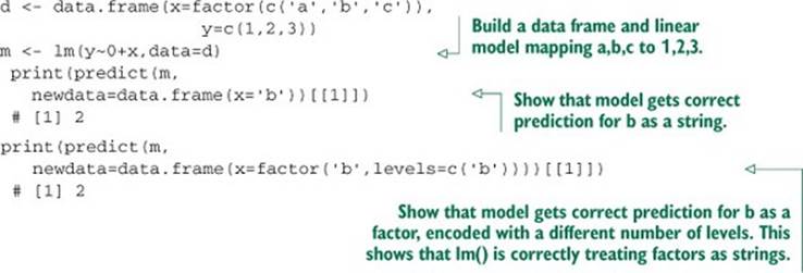
Making sure factor levels are consistent

In this book, we often prepare training and test data separately (simulating the fact that new data will be usually prepared after the original training data). For factors, this introduced two fundamental issues: consistency of numbering of factor levels during training, and application and discovery of new factor level values during application. For the first issue, it’s the responsibility of R code to make sure factor numbering is consistent. Listing A.8 demonstrates that lm() correctly handles factors as strings and is consistent even when a different set of factors is discovered during application (this is something you may want to double-check for noncore libraries). For the second issue, discovering a new factor during application is a modeling issue. The data scientist either needs to ensure this can’t happen or develop a coping strategy (such as falling back to a model not using the variable in question).

Listing A.8. Confirm lm() encodes new strings correctly.

Slots

In addition to lists, R can store values by name in object slots. Object slots are addressed with the @ operator (see help('@')). To list all of the slots on an object, try slotNames(). Slots and objects (in particular the S3 and S4 object systems) are advanced topics we won’t cover in this book. You need to know that R has object systems, as some packages will return them to you, but you shouldn’t be creating your own objects early in your R career.

A.2.3. Loading data from HTTPS sources

In chapter 2, we showed how to use read.table() to read data directly from HTTP-style URLs. With so many of our examples hosted on GitHub, it would be convenient to be able to load examples into R directly from GitHub. The difficulties in loading directly from GitHub are these: first, finding the correct URL (to avoid any GitHub page redirects), and second, finding a library that will let you access data over an HTTPS connection.

With some digging, you can work out the structure of GitHub raw URLs. And you can load data from HTTPS sources as shown in the following listing.

Listing A.9. Loading UCI car data directly from GitHub using HTTPS

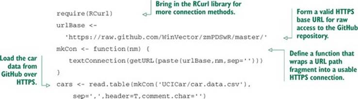
This method can be used for most of the examples in the book. But we think that cloning or downloading a zip file of the book repository is probably going to be more convenient for most readers.

A.3. Using databases with R

Some of our more significant examples require using R with a SQL database. In this section, we’ll install one such database (H2) and work one example of using SQL to process data.

A.3.1. Acquiring the H2 database engine

The H2 database engine is a serverless relational database that supports queries in SQL. All you need to do to use H2 is download the “all platforms zip” from http://www.h2database.com. Just unpack the zip file in some directory you can remember. All you want from H2 is the Java JAR file found in the unzipped bin directory. In our case, the JAR is named h2-1.3.170.jar, or you can use what comes out of their supplied installer. The H2 database will allow us to show how R interacts with a SQL database without having to install a database server. If you have access to your own database such as PostgreSQL, MySQL, or Oracle, you likely won’t need to use the H2 database and can skip it. We’ll only use the H2 database a few times in this book, but you must anticipate that some production environments are entirely oriented around a database.

A.3.2. Starting with SQuirreL SQL

SQuirreL SQL is a database browser available from http://squirrel-sql.sourceforge.net. You can use it to inspect database contents before attempting to use R. It’s also a good way to run long SQL scripts that you may write as part of your data preparation. SQuirreL SQL is also a good way to figure out database configuration before trying to connect with R. Both SQuirreL SQL and H2 depend on Java, so you’ll need a current version of Java available on your workstation (but not necessarily in your web browser, as that’s considered a security risk).

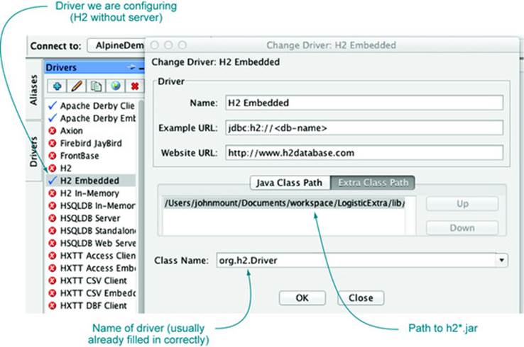
For example, we’ll show how to use SQuirreL SQL to create an example H2 database that’s visible to R. First start SQuirreL SQL, click on the Drivers pane on the right, and define a new database driver. This will bring up a panel as shown in figure A.1. We’ve selected the H2 Embedded driver. In this case, the panel comes prepopulated with the class name of the H2 driver (something we’ll need to copy to R) and what the typical structure of a URL referring to this type of database looks like. We only have to populate the Extra Class Path tab with a class path pointing to our h2-1.3.170.jar, and the driver is configured.

Figure A.1. SQuirreL SQL driver configuration

Then to connect to (and in this case create) the database, we go to the SQuirreL SQL Aliases panel and define a new connection alias, as shown in figure A.2. The important steps are to select the driver we just configured and to fill out the URL. For H2-embedded databases, the database will actually be stored as a set of files derived from the path in the specified URL.

Figure A.2. SQuirreL SQL connection alias

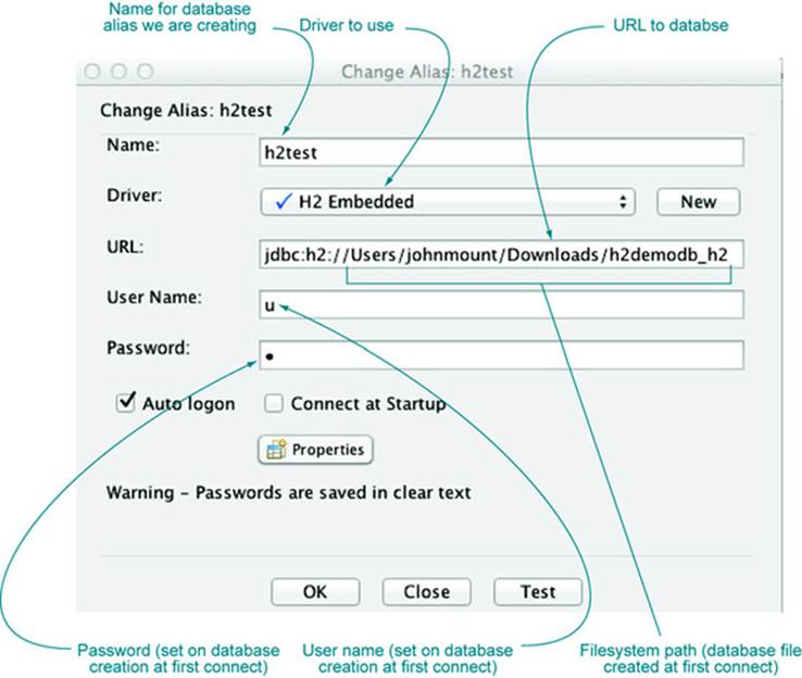
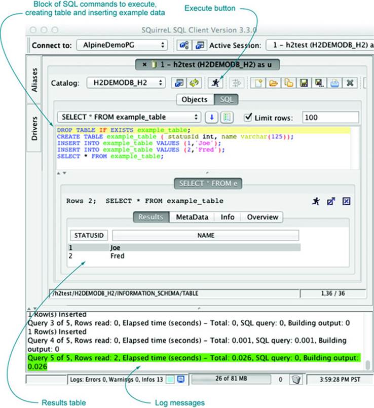
Figure A.3 shows SQuirreL SQL in action. For our example, we’re executing five lines of SQL code that create and populate a demonstration table. The point is that this same table can be easily accessed from R after we close the SQuirreL SQL connection to release the H2 exclusive lock.

Figure A.3. SQuirreL SQL table commands

To access any database from R, you can use R’s JDBC package. In the next listing, we’ll show how to do this. Each line beginning with a > prompt is a command we type into R (without copying the > prompt). Each line without the prompt is our copy of R’s response. Throughout this book, for short listings we’ll delete the prompts, and leave the prompts in when we want to demonstrate a mixture of input and output. We’ll define more of R’s syntax and commands later, but first we want to show in the following listing how to read data from our example database.

Listing A.10. Reading database data into R

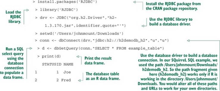
The point is this: a lot of your clients will have data in databases. One way to get at such data is to dump it into a text file like a pipe-separated values or tab-separated values file. This is often good enough, but can also lead to issues of quoting and parsing if text fields are present. Also, SQL databases carry useful schema information that provides types of various columns (not forcing you to represent numeric data as strings, which is why one of our favorite ways to move data between Python and R is the non-JDBC database SQLite). You always want the ability to directly connect to a database.

Connecting to a database can take some work, but once you get SQuirreL SQL to connect, you can copy the connection specifics (drivers, URLs, usernames, and passwords) into RJDBC and get R to connect. Some tasks, such as joins or denormalizing data for analysis, are frankly easier in SQL than in R.^[4]

⁴ Another option is to use R’s sqldf package, which allows the use of SQL commands (including fairly complicated joins and aggregations) directly on R data frames.

You’ll want to perform many data preparation steps in a database. Obviously, to use a SQL database, you need to know some SQL. We’ll explain some SQL in this book and suggest some follow-up references. We also provide a quick database data-loading tool called SQL Screwdriver.

A.3.3. Installing SQL Screwdriver

SQL Screwdriver is an open source tool for database table loading that we provide. You can download SQL Screwdriver by clicking on the Raw tab of the SQLScrewdriver.jar page found at https://github.com/WinVector/SQLScrewdriver. Every database comes with its own table dumpers and loaders, but they all tend to be idiosyncratic. SQL Screwdriver provides a single loader that can be used with any JDBC-compliant SQL database and builds a useful schema by inspecting the data in the columns of the tab- or comma-separated file it’s loading from (a task most database loaders don’t perform). We have some SQL Screwdriver documentation at http://mng.bz/bJ9B, and we’ll demonstrate SQL Screwdriver on a substantial example in this section.

A.3.4. An example SQL data transformation task

We’ll work through an artificial example of loading data that illustrates a number of R tools, including gdata (which reads Excel files) and sqldf (which implements SQL on top of R data frames). Our example problem is trying to plot the effect that room prices have on bookings for a small hotel client.

Loading data from Excel

Our data can be found in the file Workbook1.xlsx found at https://github.com/WinVector/zmPDSwR/tree/master/SQLExample. The contents of the Excel workbook look like figure A.4.

Figure A.4. Hotel data in spreadsheet form

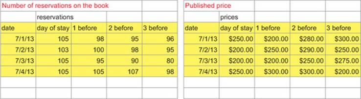
This data is typical of what you get from small Excel-oriented clients: it’s formatted for compact appearance, not immediate manipulation. The extra header lines and formatting all make the data less regular. We directly load the data into R as shown in the next listing.

Listing A.11. Loading an Excel spreadsheet

library(gdata)

bookings <- read.xls('Workbook1.xlsx',sheet=1,pattern='date',

stringsAsFactors=F,as.is=T)

prices <- read.xls('Workbook1.xlsx',sheet=2,pattern='date',

stringsAsFactors=F,as.is=T)

We confirm we have the data correctly loaded by printing it out.

Listing A.12. The hotel reservation and price data

> print(bookings)

date day.of.stay X1.before X2.before X3.before

1 2013-07-01 105 98 95 96

2 2013-07-02 103 100 98 95

3 2013-07-03 105 95 90 80

4 2013-07-04 105 105 107 98

> print(prices)

date day.of.stay X1.before X2.before X3.before

1 2013-07-01 $250.00 $200.00 $280.00 $300.00

2 2013-07-02 $200.00 $250.00 $290.00 $250.00

3 2013-07-03 $200.00 $200.00 $250.00 $275.00

4 2013-07-04 $250.00 $300.00 $300.00 $200.00

For this hotel client, the record keeping is as follows. For each date, the hotel creates a row in each sheet of their workbook: one to record prices and one to record number of bookings or reservations. In each row, we have a column labeled "day.of.stay" and columns of the form"Xn.before", which represent what was known a given number of days before the day of stay (published price and number of booked rooms). For example, the 95 bookings and $280 price recorded for the date 2013-07-01 in the column X2 before mean that for the stay date of July 1, 2013, they had 95 bookings two days before the date of stay (or on June 29, 2013) and the published price of the July 1, 2013, day of stay was quoted as $280 on June 29, 2013. The bookings would accumulate in a nondecreasing manner as we move toward the day of stay in the row, except the hotel also may receive cancellations. This is complicated, but clients often have detailed record-keeping conventions and procedures.

For our example, what the client actually wants to know is if there’s an obvious relation between published price and number of bookings picked up.

Reshaping data

For any dataset, you have keys and values. For our example of hotel booking and price data, the keys are the date (the day the customer will stay) and the number of days prior to the date the booking is made (day.of.stay, X1.before, ...). Right now, the date is a value column, but the number of days of stay is coded across many columns. The values are number of bookings and quoted prices. What we’d like to work with is a table where a specific set of columns holds keys and other columns hold values. The reshape2 package supplies a function that performs exactly this transformation, which we illustrate in the next listing.

Listing A.13. Using melt to restructure data

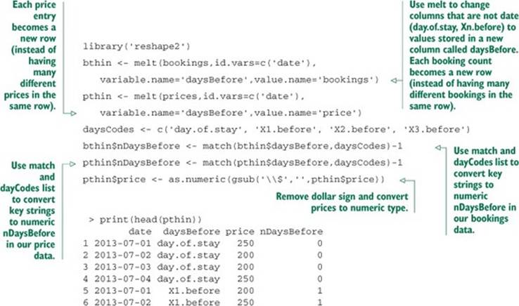
We now have our data in a much simpler and easier to manipulate form. All keys are values in rows; we no longer have to move from column to column to get different values.

Lining up the data for analysis

The bookings data is, as is typical in the hotel industry, the total number of bookings recorded for a given first day of stay. If we want to try to show the relation between price and new bookings, we need to work with change in bookings per day. To do any useful work, we have to match up three different data rows into a single new row:

· Item 1: a row from bthin supplying the total number of bookings by a given date (first day of stay) and a given number of days before the first day of stay.

· Item 2: a row from bthin supplying the total number of bookings for the same date as item 1 with nDaysBefore one larger than in item 1. This is so we can compare the two cumulative bookings and find how many new bookings were added on a given day.

· Item 3: a row from pthin supplying the price from the same date and number of days before stay as item 1. This represents what price was available at the time of booking (the decision to match this item to item 1 or item 2 depends on whether bookings are meant to record what is known at the end of the day or beginning of the day—something you need to confirm with your project sponsor).

To assemble the data, we need to use a fairly long SQL join to combine two references to bthin with one reference to pthin. While the join is complicated, notice that it specifies how we want rows to be matched up and not how to perform the matching.

Listing A.14. Assembling many rows using SQL

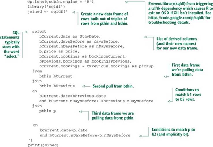
In R, there are many ways to assemble data other than SQL. But SQL commands are powerful and can be used both inside R (through sqldf) and outside R (through RJDBC).

SQL commands can look intimidating. The key is to always think about them as compositions of smaller pieces. The fact that R allows actual line breaks in string literals lets us write a large SQL command in a comparatively legible format in listing A.14 (you could even add comments using SQL’s comment mark -- where we’ve added callouts). SQL is an important topic and we strongly recommend Joe Celko’s SQL for Smarties, Fourth Edition (Morgan Kaufmann, 2011). Two concepts to become familiar with are select and join.

select

Every SQL command starts with the word select. Think of select as a scan or filter. A simple select example is select date,bookings from bthin where nDaysBefore=0. Conceptually, select scans through data from our given table (in our case bthin), and for each row matching the where clause (nDaysBefore=0) produces a new row with the named columns (date,bookings). We say conceptually because the select statement can often find all of the columns matching the where conditions much faster than a table scan (using precomputed indices). We already used simple selects when we loaded samples of data from a PUMS Census database into R.

join

join is SQL’s Swiss army knife. It can be used to compute everything from simple intersections (finding rows common to two tables) to cross-products (building every combination of rows from two tables). Conceptually, for every row in the first table, each and every row in a second table is considered, and exactly the set of rows that match the on clause is retained. Again, we say conceptually because the join implementation tends to be much faster than actually considering every pair of rows. In our example, we used joins to match rows with different keys to each other from the bthin table (called a self join) and then match to the pthin table. We can write the composite join as a single SQL statement as we did here, or as two SQL statements by storing results in an intermediate table. Many complicated calculations can be written succinctly as a few joins (because the join concept is so powerful) and also run quickly (because join implementations tend to be smart).

The purpose of this section is to show how to reshape data. But now that we’ve used select and join to build a table that relates change in bookings to known price, we can finally plot the relation in figure A.5.

Figure A.5. Hotel data in spreadsheet form

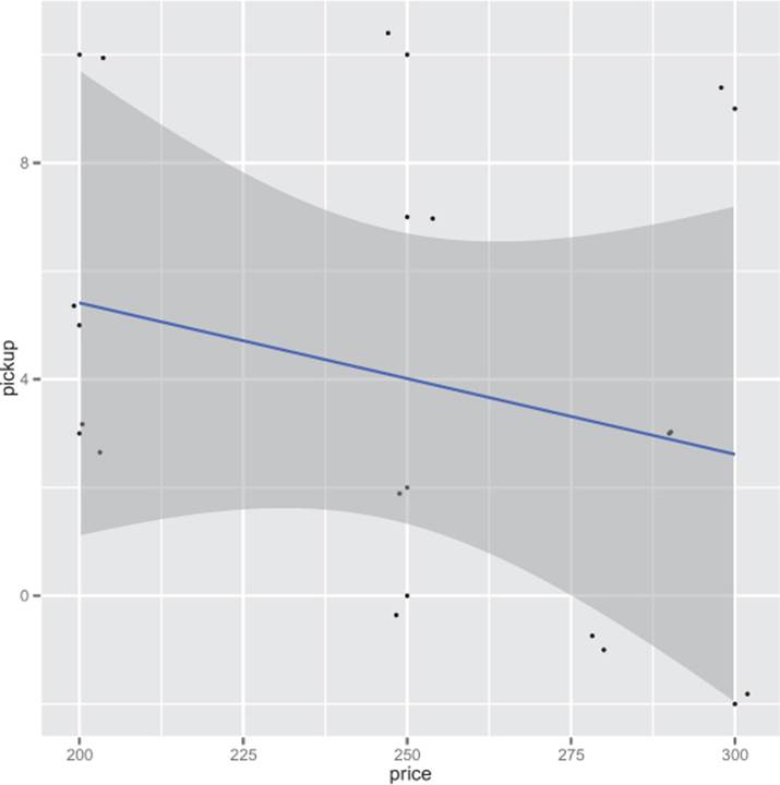
Listing A.15. Showing our hotel model results

library('ggplot2')

ggplot(data=joined,aes(x=price,y=pickup)) +

geom_point() + geom_jitter() + geom_smooth(method='lm')

print(summary(lm(pickup~price,data=joined)))

#

#Call:

#lm(formula = pickup ~ price, data = joined)

#

#Residuals:

# Min 1Q Median 3Q Max

#-4.614 -2.812 -1.213 3.387 6.386

#

#Coefficients:

# Estimate Std. Error t value Pr(>|t|)

#(Intercept) 11.00765 7.98736 1.378 0.198

#price -0.02798 0.03190 -0.877 0.401

#

#Residual standard error: 4.21 on 10 degrees of freedom

#Multiple R-squared: 0.07144, Adjusted R-squared: -0.02142

#F-statistic: 0.7693 on 1 and 10 DF, p-value: 0.401

The first thing to notice is the model coefficient p-value on price is way too large. At 0.4, the estimated relation between price and change in bookings can’t be trusted. Part of the problem is we have very little data: the joined data frame only has 12 rows. Also, we’re co-mingling data from different numbers of days before stay and different dates without introducing any features to model these effects. And this type of data is likely censored because hotels stop taking reservations as they fill up, independent of price. Finally, it’s typical of this sort of problem for the historic price to actually depend on recent bookings (for example, managers drop prices when there are no bookings), which can also obscure an actual causal connection from price to bookings. For an actual client, the honest report would say that to find a relation more data is needed. We at least need to know more about hotel capacity, cancellations, and current pricing policy (so we can ensure some variation in price and eliminate confounding effects from our model). These are the sort of issues you’d need to address in experiment design and data collection.

A.3.5. How to think in SQL

The trick to thinking in SQL is this: for every table, classify the columns into a few important themes and work with the natural relations between these themes. One view of the major column themes is given in the table A.1.

Table A.1. Major SQL column themes

The point is that analysis is much easier if you have a good taxonomy of column themes for every supplied data source. You then design SQL command sequences to transform your data into a new table where the columns are just right for analysis (as we demonstrated in section A.3.4). In the end, you should have tables where every row is an event you’re interested in and every needed fact is already available in a column. Building temporary tables and adding columns is much better than having complicated analysis code. These ideas may seem abstract, but they guide the analyses in this book.