Network Security Through Data Analysis: Building Situational Awareness (2014)

Part III. Analytics

Chapter 15. Network Mapping

In this chapter, we discuss mechanisms for managing the rate of false positives produced by detection systems by reducing make-work. Consider this scenario: I create a signature today to identify the IIS exploit of the week, and sometime tomorrow afternoon it starts firing off like crazy. Yay, somebody’s using an exploit! I check the logs, and I find out that I am not in fact being attacked by this exploit because my network actually doesn’t run IIS. Not only have I wasted analyst time dealing with the alert, I’ve wasted my time writing the original alert for something to which the network isn’t vulnerable.

The process of inventory is the foundation of situational awareness. It enables you to move from simply reacting to signatures to continuous audit and protection. It provides you with baselines and an efficient anomaly detection strategy, it identifies critical assets, and it provides you with contextual information to speed up the process of filtering alerts.

Creating an Initial Network Inventory and Map

Network mapping is an iterative process that combines technical analysis and interviews with site administrators. The theory behind this process is that any inventory generated by design is inaccurate to some degree, but accurate enough to begin the process of instrumentation and analysis. Acquiring this inventory begins with identifying the personnel responsible for managing the network.

The mapping process described in this book consists of four distinct phases, which combine iterative traffic analysis and asking a series of questions of network administrators and personnel. These questions inform the traffic analyses, and the analyses lead to more queries. Figure 15-1 shows how the process progresses: in phase I, you identify the space of IP addresses you are monitoring, and in each progressive phase you partition the space into different categories.

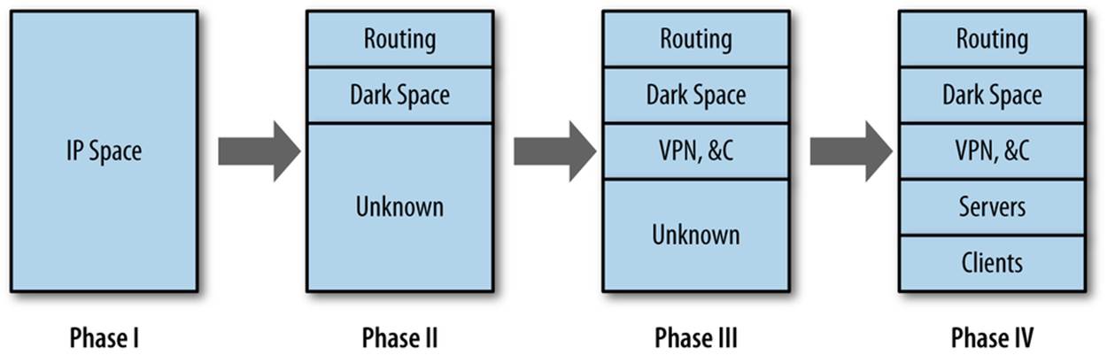
Figure 15-1. The mapping process

Creating an Inventory: Data, Coverage, and Files

In a perfect world, a network map should enable you to determine, based on addresses and ports, the traffic you are seeing on any host on the network. The likelihood of producing such a perfect map on an enterprise network is pretty low because by the time you finish the initial inventory,something on the network will have changed. Maps are dynamic and consequently have to be updated on a regular basis. This updating process provides you with a facility for continuously auditing the network.

A security inventory should keep track of every addressable resource on the network (that is, anything an attacker could conceivably reach if she had network access, even if that means access inside the network). It should keep track of which services are running on the resource, and it should keep track of how that system is monitored. An example inventory is shown in Table 15-1.

Table 15-1. An example worksheet

Table 15-1 has an entry for each unique observed port and protocol combination on the network, along with a role, an indicator of when the host was last seen in the sensor data, and the available sensor information. These fields are the minimum set that you should consider if generating an inventory. Additional potential items to consider include the following:

§ The Role field should be enumerable, rather than an actual text field. Enumerating the roles will make searching much less painful. A suggested set of categories is:

§ Service Server, where Service is HTTP, SSH, etc.

§ Workstation, to indicate a dedicated client

§ NAT, to indicate a network address translator

§ Service Proxy for any proxies

§ Firewall for Firewalls

§ Sensor for any sensors

§ Routing for any routing equipment

§ VPN for VPN concentrators and other equipment

§ DHCP for any dynamically addressed space

§ Dark for any address that is allocated in the network but has no host on it

§ Identifying VPNs, NATs, DHCP, and proxies, as we’ll discuss in a moment, is particularly important—they mess up the address allocation and increase the complexity of analysis.

§ Keeping centrality or volume metrics is also useful. A five-number summary of volume over a month is a good starting point for anomaly detection.

§ Per-host whitelists are a useful tool for anomaly management (see Chapter 2 for a more extensive discussion). The inventory is a good place to track per-host whitelist and rule files.

§ Ownership and point of contact information is critical. One of the most time-consuming steps after identifying an attack is usually finding out who owns the victim.

§ Keeping track of the specific services on hosts, and the versions of those services, helps track the risk that a particular system has to current exploits. This can be identified by banner grabbing, but it’s more effective to just scan the network using the inventory as a guideline.

Table 15-1 could be kept on paper or a spreadsheet, but it really should be kept in an RDBMS or other storage system. Once you’ve created the inventory, it will serve as a simple anomaly detection system, and should be updated regularly by automated processes.

Phase I: The First Three Questions

The first step of any inventory process involves figuring out what is already known and what is already available for monitoring. For this reason, instrumentation begins at a meeting with the network administrators.^[25^] The purpose of this initial meeting is to determine what is monitored, specifically:

§ What addresses make up the network?

§ What sensors do I have?

§ How are the sensors related to traffic?

Start with addresses, because they serve as the foundation of the inventory. More specific questions to ask include:

Is the network IPv4 or IPv6?

If the network is IPv6, there’s going to be a lot more address space to play with, which reduces the need for DHCP and NAT. The network is more likely to be IPv4, however, and that means that if it is of any significant size, there’s likely to be a fair degree of aliasing, NAT, and other address conservation tricks.

How many addresses are accessible or hidden behind NATs?

Ideally, you should be able to get a map showing the routing on the network, whether there are DMZs, and what information is hidden behind NATs. These individual subnets are future candidates for instrumentation.

How many hosts are on the network?

Determine how many PCs, clients, servers, computers, and embedded systems are on the network. These systems are the things you’re defending. Pay particular attention to embedded systems such as printers and teleconferencing tools because they often have network servers, are hard to patch and update, and are often overlooked in inventories.

This discussion should end with a list of all your potential IP addresses. This list will probably include multiple instances of the same ephemeral spaces over and over again. For example, if there are six subnets behind NAT firewalls, expect to see 192.168.0.0/16 repeated six times. You should also get an estimate of how many hosts are in each subnet and in the network as a whole.

The next set of questions to ask involves current instrumentation. Host-based instrumentation (e.g., server logs and the like, as discussed in Chapter 3) are not the primary target at this point. Instead, the goal is to identify whether network-level collection is available. If it is available, determine what is collected, and if not, determine whether it can be turned on. More specific questions to ask include:

What is currently being collected?

A source doesn’t have to be collected “for security purposes” to be useful. NetFlow, for example, has been primarily used as a billing system, but can be useful in monitoring as well.

Are there NetFlow-capable sensors?

For example, if Cisco routers with built-in NetFlow instrumentation are available, use them as your initial sensors.

Is any IDS present?

An IDS such as Snort can be configured to just dump packet headers. Depending on the location of the IDS (such as if it’s on the border of a network), it may be possible to put up a flow collector there as well.

At the conclusion of this discussion, you should come up with a plan for initially instrumenting the network. The goal of this initial instrumentation should be to capitalize on any existing monitoring systems and to acquire a systematic monitoring capability for cross-border traffic. As a rule of thumb, on most enterprise networks, it’s easiest to turn on deactivated capabilities such as NetFlow, while it’s progressively more difficult, respectively, to add new software and hardware.

The Default Network

Throughout this chapter, I use sidebars to discuss more concrete methods to answer the high-level questions in the text. These sidebars involve a hefty number of SiLK queries and at least a little understanding of how SiLK breaks down data.

The default network is shown in Figure 15-2. As described by SiLK, this network as two sensors: R1 (Router 1) and R2 (Router 2). There are three types of data: in (coming from the cloud into the network), out (going from the network to the cloud), and internal (traffic that doesn’t cross the border into the cloud).

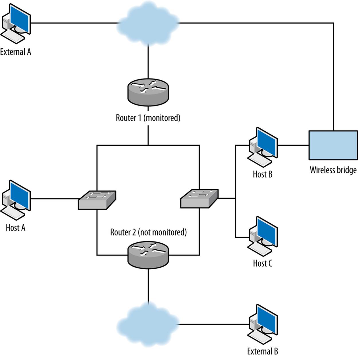
Figure 15-2. Unmonitored routes in action

In addition, there exist a number of IP sets. initial.set is a list of hosts on the network provided by administrators during the initial interview. This set is composed of servers.set and clients.set, comprising the clients and servers. servers.set contains webservers.set,dnsservers.set, and sshservers.set as subsets. These sets are accurate at the time of the interview, but will be updated as time passes.

Phase II: Examining the IP Space

You’ll need to consider the following questions:

§ Are there unmonitored routes?

§ What IP space is dark?

§ Which IP addresses are network appliances?

Following phase I, you should have an approximate inventory of the network and a live feed of, at the minimum, cross-border traffic data. With this information, you can begin to validate the inventory by comparing the traffic you are receiving against the list of IP addresses that the administrators provided you. Note the use of the word validate—you are comparing the addresses that you observe in traffic against the addresses you were told would be there.

Your first goal is to determine whether instrumentation is complete or incomplete, in particular, whether you have any unmonitored routes to deal with—that is, legitimate routes where traffic is not being recorded. Figure 15-2 shows some common examples of dark routes. In this figure, a line indicates a route between two entities:

§ The first unmonitored route occurs when traffic moves through router 2, which is not monitored. For example, if host A communicates with external address B using router 2, you will not see A’s traffic to B or B’s traffic to A.

§ A more common problem in modern networks is the present of wireless bridges. Most modern hosts have access to multiple wireless networks, especially in shared facilities. Host B in the example can communicate with the Internet while bypassing router 1 entirely.

The key to identifying unmonitored routes is to look at asymmetric traffic flow. Routing protocols forward traffic with minimal interest in the point of origin, so if you have n access points coming into your network, the chance of any particular session going in and out of the same point is about 1/n. You can expect some instrumentation failures to result on any network, so there are always going to be broken sessions, but if you find consistent evidence of asymmetric sessions between pairs of addresses, that’s good evidence that the current monitoring configuration is missing something.

The best tool for finding asymmetric sessions is TCP traffic, because TCP is the most common protocol in the IP suite that guarantees a response. To identify legitimate TCP sessions, take the opposite approach from Chapter 11: look for sessions where the SYN, ACK, and FIN flags are high, with multiple packets or with payload.

Identifying Asymmetric Traffic

To identify asymmetric traffic, look for TCP sessions that carry payload and don’t have a corresponding outgoing session. This can be done using rwuniq and rwfilter:

$ rwfilter --start-date=2013/05/10:00 --end-date=2013/05/10:00 --proto=6 \

--type=out --packets=4- --flags-all=SAF/SAF --pass=stdout | \

rwuniq --field=1,2 --no-title --sort | cut -d '|' -f 1,2 > outgoing.txt

# Note that I use 1,2 for the rwuniq above, and 2,1 for the rwuniq below.

# This ensures that the

# fields are present in the same order when I compare output.

$ rwfilter --start-date=2013/05/10:00 --end-date=2013/05/10:00 --proto=6 \

--type=in --packets=4- --flags-all=SAF/SAF --pass=stdout | rwuniq \

--field=2,1 --no-title --sort | cut -d '|' -f 2,1 > incoming.txt

Once these commands finish, I will have two files of internal IP and external IP pairs. I can compare these pairs directly using -cmp or a hand-written routine. Example 15-1 shows a python example that generates a report of unidirectional flows:

Example 15-1. Generating a report of unidirectional flows

#!/usr/bin/env python

#

#

# compare_reports.py

#

# Command line: compare_reports.py file1 file2

#

# Reads the contents of two files and checks to see if the same

# IP pairs appear.

#

import sys, os

def read_file(fn):

ip_table = set()

a = open(fn,'r')

for i in a.readlines():

sip, dip = map(lambda x:x.strip(), i.split('|')[0:2])

key = "%15s:%15s" % (sip, dip)

ip_table.add(key)

a.close()

return ip_table

if __name__ == '__main__':

incoming = read_file(sys.argv[1])

outgoing = read_file(sys.argv[2])

missing_pairs = set()

total_pairs = set()

# Being a bit sloppy here, run on both incoming and outgoing to ensure

# that if there's an element in one not in the other, it gets caught

for i in incoming:

total_pairs.add(i)

if not i in outgoing:

missing_pairs.add(i)

for i in outgoing:

total_pairs.add(i)

if not i in incoming:

missing_pairs.add(i)

print missing_pairs, total_pairs

# Now do some address breakdowns

addrcount = {}

for i in missing_pairs:

in_value, out_value = i.split(':')[0:2]

if not addrcount.has_key(in_value):

addrcount[in_value] = 0

if not addrcount.has_key(out_value):

addrcount[out_value] = 0

addrcount[in_value] += 1

addrcount[out_value] += 1

# Simple report, number of missing pairs, list of most commonly occurring

# addresses

print "%d missing pairs out of %d total" % (len(missing_pairs),

len(total_pairs))

s = addrcount.items()

s.sort(lambda a,b:b[1] - a[1]) # lambda just guarantees order

print "Most common addresses:"

for i in s[0:10]:

print "%15s %5d" % (i[0],addrcount[i[0]])

This approach is best done using passive collection because it ensures that you are observing traffic from a number of locations outside the network. Scanning is also for identifying dark spaces and back doors. When you scan and control the instrumentation, not only can you see the results of your scan on your desktop, but you can compare the traffic from the scan against the data provided by your collection system.

Although you can scan the network and check whether all your scanning sessions match your expectations (i.e., you see responses from hosts and nothing from empty space), you are scanning from only a single location, when you really need to look at traffic from multiple points of origin.

If you find evidence of unmonitored routes, you need to determine whether they can be instrumented and why they aren’t being instrumented right now. Unmonitored routes are a security risk: they can be used to probe, exfiltrate, and communicate without being monitored.

Unmonitored routes and dark spaces have similar traffic profiles to each other; in both cases, a TCP packet sent to them will not elicit a reply. The difference is that in an unmonitored route, this happens due to incomplete instrumentation, while a dark space has nothing to generate a response. Once you have identified your unmonitored routes, any monitored addresses that behave in the same way should be dark.

Identifying Dark Space

Dark spaces can be found either passively or actively. Passive identification requires collecting traffic to the network and progressively eliminating all address that respond or are unmonitored—at that point, the remainder should be dark. The alternative approach is to actively probe the addresses in a network and record the ones that don’t respond; those addresses should be dark.

Passive collection requires gathering data over a long period. At the minimum, collect traffic for at least a week to ensure that dynamic addressing and business processes are handled.

$ rwfilter --type=out --start-date=2013/05/01:00 --end-date=2013/05/08:23 \

--proto=0-255 --pass=stdout | rwset --sip-file=light.set

# Now remove the lit addresses from our total inventory

$ rwsettool --difference --output=dark.set initial.set light.set

An alternative approach is to ping every host on the network to determine whether it is present.

$ for i in `rwsetcat initial.set`

do

# Do a ping with a 5 second timeout and 1 attempt to each target

ping -q -c 1 -t 5 ${i} | tail -2 >> pinglog.txt

done

pinglog.txt will contain the summary information from the ping command, which will look like this:

--- 128.2.11.0 ping statistics ---

1 packets transmitted, 0 packets received, 100.0% packet loss

The contents can be parsed to produce a dark map.

Of these two options, scanning will be faster than passive mapping, but you have to make sure the network will return ECHO REPLY ICMP messages to your pings.

Another way to identify dynamic spaces through passive monitoring is to take hourly pulls and compare the configuration of dark and light addresses in each hour.

“Network appliances” in this context really means router interfaces. Router interfaces are identifiable by looking for routing protocols such as BGP, RIP, and OSPF. Another mechanism to use is to check for “ICMP host not found” messages (also known as network unreachable messages), which are generated only by routers.

Finding Network Appliances

Identifying network appliances involves either using traceroute, or looking for specific protocols used by them. Every host mentioned by traceroute except the endpoint is a router. If you check for protocols, candidates include:

BGP

BGP is commonly spoken by routers that route traffic across the Internet, and won’t be common inside corporate networks unless you have a very big network. BGP runs on TCP port 179.

# This will identify communications from the outside world with BGP speakers

# inside.

$ rwfilter --type=in --proto=6 --dport=179 --flags-all=SAF/SAF \

--start-date=2013/05/01:00 --end-date=2013/05/01:00 --pass=bgp_speakers.rwf

OSPF and EIGRP

Common protocols for managing routing on small networks. EIGRP is protocol number 88, OSPF protocol number 89.

# This will identify communications between OSPF and EIGRP speakers,

# note the use of internal, we don't expect this traffic to be cross-border

$ rwfilter --type=internal --proto=88,89 --start-date=2013/05/01:00 \

--end-date=2013/05/01:00 --pass=stdout | rwfilter --proto=88 \

--input-pipe=stdin --pass=eigrp.rwf --fail=ospf.rwf

RIP

Another internal routing protocol, RIP is implemented on top of UDP using port 520.

# This will identify communications with RIP speakers

$ rwfilter --type=internal --proto=17 --aport=520 \

--start-date=2013/05/01:00 --end-date=2013/05/01:00 --pass=rip_speakers.rwf

ICMP

Host unreachable messages (ICMP Type 3, Code 7) and time exceeded messages (ICMP Type 11) both originate from routers.

# Filter out icmp messages, the longer period is because ICMP is much rarer

$ rwfilter --type=out --proto=1 --icmp-type=3,11 --pass=stdout \

--start-date=2013/05/01:00 \

--end-date=2013/05/01:23 | rwfilter --icmp-type=11 --input-pipe=stdin \

--pass=ttl_exceeded.rwf --fail=stdout | rwfilter --input-pipe=stdin \

--icmp-code=7 --pass=not_found.rwf

$ rwset --sip=routers_ttl.set ttl_exceeded.rwf

$ rwset --sip=routers_nf.set not_found.rwf

$ rwsettool --union --output-path=routers.set routers_nf.set routers_ttl.set

The results of this step will provide you with a list of router interface addresses. Each router on the network will control one or more of these interfaces. At this point, it’s a good idea to go back to the network administrators in order to associate these interfaces with actual hardware.

Phase III: Identifying Blind and Confusing Traffic

You’ll need to consider the following questions:

§ Are there NATs?

§ Are there proxies, reverse proxies, or caches?

§ Is there VPN traffic?

§ Are there dynamic addresses?

After completing phase II, you will have identified which addresses within your network are active. The next step is to identify which addresses are going to be problematic. Life would be easier for you if every host were assigned a static IP address, that address were used by exactly one host, and the traffic were easily identifiable by port and protocol.

Obviously, these constraints don’t hold. Specific problems include:

NATs

These are a headache because they alias multiple IP addresses behind a much smaller set of addresses.

Proxies, reverse proxies, and caches

Like a NAT, a proxy hides multiple IP addresses behind a single proxy host address. Proxies generally operate at higher levels in the OSI stack and often handle specific protocols. Reverse proxies, as the name implies, provide aliases for multiple server addresses and are used for load balancing and caching. Caches store repeatedly referenced results (such as web pages) to improve performance.

VPNs

Virtual Private Network (VPN) traffic obscures the contents of protocols, hiding what’s being done and hiding how many hosts are involved. VPN traffic includes IPv6-over-IPv4 protocols such as 6to4 and Teredo, and encrypted protocols such as SSH and TOR. All of these protocols encapsulate traffic, meaning that the addresses seen at the IP layer are relays, routers, or concentrators rather than the actual hosts doing something.

Dynamic addresses

Dynamic addressing, such as that assigned through DHCP, causes a single host to migrate through a set of addresses over time. Dynamic addressing complicates analysis by introducing a lifetime for each address. You can never be sure whether the host you’re tracking through its IP address did something after its DHCP lease expired.

These particular elements should be well-documented by network administrators, but there are a number of different approaches for identifying them. Proxies and NATs can both be identified by looking for evidence that a single IP address is serving as a frontend for multiple addresses. This can be done via packet payload or flow analysis, although packet payload is more certain.

Identifying NATs

NATs are an enormous pain to identify unless you have access to payload data, in which case they simply become a significant pain. The best approach for identifying NATs is to quiz the network administrators. Failing that, you have to identify NATs through evidence that there are multiple addresses hidden behind the same address. A couple of different indicia can be used for this.

Variant User-Agent strings

The best approach I’ve seen to identify NAT is to pull the User-Agent strings from web sessions. Using a script such as bannergrab.py from Chapter 14, you can pull and dump all instances of the User-Agent string issuing from the NAT. If you see different instances of the same browser, or multiple browsers, you are likely looking at a NAT.

There is a potential false positive here. A number of applications (including email clients) include some form of HTTP interaction these days. Consequently, it’s best to restrict yourself to explicit browser banners, such as those output by Firefox, IE, Chrome, and Opera.

Multiple logons to common servers

Identify major internal and external services used by your network. Examples include the company email server, Google, and major newspapers. If a site is a NAT, you should expect to see redundant logins from the same address. Email server logs and internal HTTP server logs are the best tool for this kind of research.

TTL behavior

Recall that time-to-live (TTL) values are assigned by the IP stack and that initial values are OS-specific. Check the TTLs coming from a suspicious address and see if they vary. Variety suggests multiple hosts behind the address. If values are the same but below the initial TTL for an OS, you’re seeing evidence of multiple hops to reach that address.

Identifying Proxies

Proxy identification requires you to have both sides of the proxy instrumented. Figure 15-3 shows the network traffic between clients, proxies, and servers. As this figure shows, proxies take in requests from multiple clients, and send those requests off to multiple servers. In this way, a proxy behaves as both a server (to the clients it’s proxying for) and as a client (to the servers it’s proxying to). If your instrumentation lets you see both the client-to-proxy and proxy-to-server communication, you can identify the proxy by viewing this traffic pattern. If you don’t, you can use the techniques discussed in the previous cookbook on NAT identification. The same principles apply because, after all, a proxy is a frontend to multiple clients like a NAT firewall.

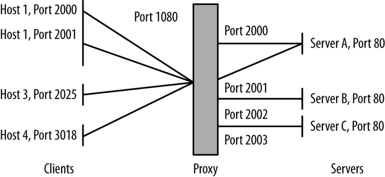
Figure 15-3. Network connections for a proxy

To identify a proxy using its connectivity, first look for hosts that are acting like clients. You can tell a client because it uses multiple ephemeral ports. For example, using rwuniq, you can identify clients on your network as follows:

$ rwfilter --type=out --start-date=2013/05/10:00 --end-date=2013/05/10:01 \

--proto=6,17 --sport=1024-65535 --pass=stdout | rwuniq --field=1,3 \

--no-title | cut -d '|' -f 1 | sort | uniq -c | egrep -v '^[ ]+1' |\

cut -d ' ' -f 3 | rwsetbuild stdin clients.set

That command identifies all combinations of source IP address (sip) and source port number (sport) in the sample data and eliminates any situation where a host only used one port. The remaining hosts are using multiple ports. It’s possible that hosts that are using only seven or eight ports at a time are running multiple servers, but as the distinct port count rises, the likelihood of them running multiple services drops.

Once you’ve identified clients, the next step is to identify which of the clients are also behaving as servers (see Identifying Servers).

VPN traffic can be identified by looking for the characteristic ports and protocols used by VPNs. VPNs obscure traffic analysis by wrapping all of the traffic they transport in another protocol such as GRE. Once you’ve identified a VPN’s endpoints, instrument there. Once the wrapper has been removed from VPN traffic, you should be able to distinguish flows and session data.

Identifying VPN Traffic

The major protocols and ports used by VPN traffic are:

IPSec

IPSec refers to a suite of protocols for encrypted communications over VPNs. The two key protocols are AH (authentication header, protocol 51) and ESP (Encapsulating Security Payload, protocol 50):

$ rwfilter --start-date=2013/05/13:00 --end-date=2013/05/13:01 --proto=50,51 \

--pass=vpn.rwf

GRE

GRE (generic routing encapsulation) is the workhorse protocol for a number of VPN implementations. It can be identified as protocol 47.

$ rwfilter --start-date=2013/05/13:00 --end-date=2013/05/13:01 --proto=47 \

--pass=gre.rwf

A number of common tunneling protocols are also identifiable using port and protocol numbers, although unlike standard VPNs, they are generally software-defined and don’t require special assets specifically for routing. Examples include SSH, Teredo, 6to4, and TOR.

Phase IV: Identifying Clients and Servers

After identifying the basic structure of the network, the next step is to identify what the network does, which requires profiling and identifying clients and servers on the network. Questions include:

§ What are the major internal servers?

§ Are there servers running on unusual ports?

§ Are there FTP, HTTP, SMTP, or SSH servers that are not known to system administration?

§ Are servers running as clients?

§ Where are the major clients?

Identifying Servers

Servers can be identified by looking for ports that receive sessions and by looking at the spread of communications to ports.

To identify ports that are receiving sessions, you need either access to pcap data or flow instrumentation that distinguishes the initial flags of a packet from the rest of the body (which you can get through YAF, as described in YAF). In a flow, the research then becomes a matter of identifying hosts that respond with a SYN and ACK:

$ rwfilter --proto=6 --flags-init=SA|SA --pass=server_traffic.rwf \

--start-date=2013/05/13:00 --end-date=2013/05/13:00 --type=in

This approach won’t work with UDP, because a host can send UDP traffic to any port it pleases without any response. An alternate approach, which works with both UDP and TCP, is to look at the spread of a port/protocol combination. I briefly touched on this in Identifying Proxies, and we’ll discuss it in more depth now.

A server is a public resource. This means that the address has to be sent to the clients, and that, over time, you can expect multiple clients to connect to the server’s address. Therefore, over time, you will see multiple flows with distinct source IP/source port combinations all communicating with the same destination IP/destination port combination. This differs from the behavior of a client, which will issue multiple sessions from different source ports to a number of distinct hosts. Figure 15-4 shows this phenomenon graphically.

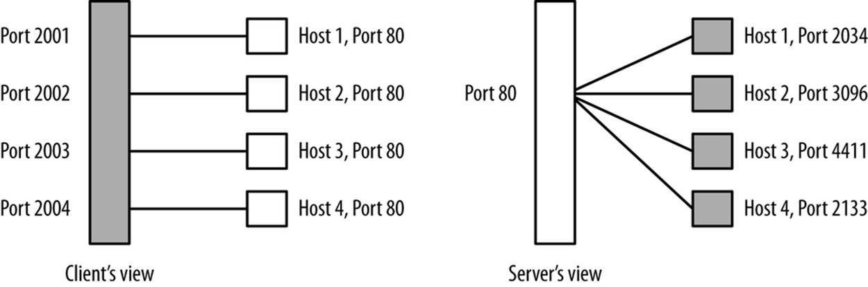
Figure 15-4. A graphical illustration of spread

Spread can easily be calculated with flow data by using the rwuniq command. Given a candidate file of traffic originating from one IP address, use the following:

$rwuniq --field=1,2 --dip-distinct candidate_file | sort -t '|' -k3 -nr |\

head -15

The more distinct IP addresses talk to the same host/port combination, the more likely is it that the port represents a server. In this script, servers will appear near the top of the list.

By using spread and direct packet analysis, you should have a list of most of the IP:port combinations that are running servers. This is always a good time to scan those IP:port combinations to verify what’s actually running: in particular, search for servers that are not running on common ports. Servers are a public resource (for some limited definition of “public”), and when they appear on an unusual port, it may be an indication that a user didn’t have permissions to run the server normally (suspicious behavior) or was trying to hide it (also suspicious behavior, especially if you’ve read Chapter 11).

Once you’ve identified the servers on a network, determine which ones are most important. There are a number of different metrics for doing so, including:

Total volume over time

This is the easiest and most common approach.

Internal and external volume

This differentiates servers accessed only by your own users from those accessed by the outside world.

Graph centrality

Path and degree centrality often identify hosts that are important and that would be missed using pure degree statistics (number of contacts). See Chapter 13 for more information.

The goal of this exercise is to produce a list of servers ordered by priority, from the ones you should watch the most to the ones that are relatively low profile or, potentially, even removable.

Once you have identified all the servers on a network, it’s a good time to go back to talk to the network administrators.^[26^] This is because you will almost invariably find servers that nobody knew were running on the network, examples of which include:

§ Systems being run by power users

§ Embedded web servers

§ Occupied hosts

Identifying Sensing and Blocking Infrastructure

Questions to consider:

§ Are there any IDS or IPS systems in place? Can I modify their configuration?

§ What systems do I have log access to?

§ Are there any firewalls?

§ Are there any router ACLs?

§ Is there an antispam system at the border, or is antispam handled at the mail server, or both?

§ Is AV present?

The final step of any new instrumentation project is to figure out what security software and capabilities are currently present. In many cases, these systems will be identifiable more from an absence than a presence. For example, if no hosts on a particular network show evidence of BitTorrent traffic (ports 6881–6889), it’s likely that a router ACL is blocking BitTorrent.

Updating the Inventory: Toward Continuous Audit

Once you’ve built an initial inventory, queue up all the analysis scripts you’ve written to run on a regular basis. The goal is to keep track of what’s changed on your network over time.

This inventory provides a handy anomaly-detection tool. The first and most obvious approach is to keep track of changes in the inventory. Sample questions to ask include:

§ Are there new clients or servers on the network?

§ Have previously existing addresses gone dark?

§ Has a new service appeared on a client?

Changes in the inventory can be used as triggers for other analyses. For example, when a new client or server appears on the network, you can start analyzing its flow data to see who it communicates with, scan it, or otherwise experiment on it in order to fill the inventory with information on the new arrival.

In the long term, keeping track of what addresses are known and monitored is a first approximation for how well you’re protecting the network. It’s impossible to say “X is more secure than Y”; we just don’t have the ability to quantitatively measure the X factor that is attacker interest. By working with the map, you can track coverage either as a strict number (out of X addresses on the network, Y are monitored) or as a percentage.

Further Reading

1. Umesh Shankar and Vern Paxson, “Active Mapping: Resisting NIDS Evasion Without Altering Traffic,” Proceedings of the 2003 IEEE Symposium on Security and Privacy.

2. Austin Whisnant and Sid Faber, “Network Profiling Using Flow,” CMU/SEI-2012-TR-006, Software Engineering Institute.