Software Testing Foundations: A Study Guide for the Certified Tester Exam (2014)

Chapter 5. Dynamic Analysis - Test Design Techniques

This chapter describes techniques for testing software by executing the test objects on a computer. It presents the different techniques, with examples, for specifying test cases and for defining test exit criteria.

These →test design techniques are divided into three categories: black box testing, white box testing, and experience-based testing.

Execution of the test object on a computer

Usually, testing of software is seen as the execution of the test object on a computer. For further clarification, the phrase →dynamic analysis is used. The test object (program) is fed with input data and executed. To do this, the program must be executable. In the lower test stages (component and integration testing), the test object cannot be run alone but must be embedded into a test harness or test bed to obtain an executable program (see figure 5-1).

A test bed is necessary

The test object will usually call different parts of the program through predefined interfaces. These parts of the program are represented by placeholders called stubs when they are not yet implemented and therefore aren’t ready to be used or if they should be simulated for this particular test of the test object. Stubs simulate the input/output behavior of the part of the program that usually would be called by the test object.¹

Figure 5–1
Test bed

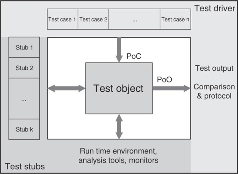
Furthermore, the test bed must supply the test object with input data. In most cases, it is necessary to simulate a part of the program that is supposed to call the test object. A test driver does this. Driver and stub combined establish the test bed. Together, they constitute an executable program with the test object itself.

The tester must often create the test bed, or the tester must expand or modify standard (generic) test beds, adjusting them to the interfaces of the test object. Test bed generators can be used as well (see section 7.1.4). An executable test object makes it possible to execute the dynamic test.

Systematic approach for determining the test cases

The objective of testing is to show that the implemented test object fulfills specified requirements as well as to find possible faults and failures. With as little cost as possible, as many requirements as possible should be checked and as many failures as possible should be found. This goal requires a systematic approach to test case design. Unstructured testing “from your gut feeling” does not guarantee that as many as possible, maybe even all, different situations supported by the test object are tested.

Step wise approach

The following steps are necessary to execute the tests:

§ Determine conditions and preconditions for the test and the goals to be achieved.

§ Specify the individual test cases.

§ Determine how to execute the tests (usually chaining together several test cases).

This work can be done very informally (i.e., undocumented) or in a formal way as described in this chapter. The degree of formality depends on several factors, such as the application area of the system (for example, safety-critical software), the maturity of the development and test process, time constraints, and knowledge and skill level of the project participants, just to mention a few.

Conditions, preconditions, and goals

At the beginning of this activity, the test basis is analyzed to determine what must be tested (for example, that a particular transaction is correctly executed). The test objectives are identified, for example, demonstrating that requirements are met. The failure risk should especially be taken into account. The tester identifies the necessary preconditions and conditions for the test, such as what data should be in a database.

Traceability

The traceability between specifications and test cases allows an analysis of the impact of the effects of changed specifications on the test, that is, the necessity for creation of new test cases and removal or change of existing ones. Traceability also allows checking a set of test cases to see if it covers the requirements. Thus, coverage can be a criterion for test exit.

In practice, the number of test cases can soon reach hundreds or thousands. Only traceability makes it possible to identify the test cases that are affected by specification changes.

→Test case specification

Part of the specification of the individual test cases is determining test input data for the test object. They are determined using the methods described in this chapter. However, the preconditions for executing the test case, as well as the expected results and expected postconditions, are necessary for determining if there is a failure (for detailed descriptions, see [IEEE 829]).

Determining expected result and behavior

The expected results (output, change of internal states, etc.) should be determined and documented before the test cases are executed. Otherwise, an incorrect result can easily be interpreted as correct, thus causing a failure to be overlooked.

Test case execution

It does not make much sense to execute an individual test case. Test cases should be grouped in such a way that a whole sequence of test cases is executed (test sequence, test suite or test scenario). Such a test sequence is documented in the →test procedure specifications or test instructions. This document commonly groups the test cases by topic or by test objectives. Test priorities and technical and logical dependencies between the tests and regression test cases should be visible. Finally, the test execution schedule (assigning tests to testers and determining the time for execution) is described in a →test schedule document.

To be able to execute a test sequence, a →test procedure or →test script is required. A test script contains instructions for automatically executing the test sequence, usually in a programming language or a similar notation, the test script may contain the corresponding preconditions as well as instruction for comparing the actual and expected results. JUnit is an example of a framework that allows easy programming of test scripts in Java [URL: xunit].

Black box and white box test design techniques

Several different approaches are available for designing tests. They can roughly be categorized into two groups: black box techniques² and white box techniques³. To be more precise, they are collectively called test case design techniques because they are used to design the respective test cases.

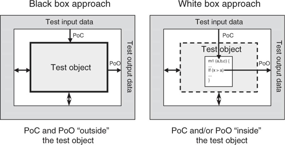
In black box testing, the test object is seen as a black box. Test cases are derived from the specification of the test object; information about the inner structure is not necessary or available. The behavior of the test object is watched from the outside (the →Point of Observation, or PoO, is outside the test object). The operating sequence of the test object can only be influenced by choosing appropriate input test data or by setting appropriate preconditions. The →Point of Control (PoC) is also located outside of the test object. Test cases are designed using the specification or the requirements of the test object. Often, formal or informal models of the software or component specification are used. Test cases can be systematically derived from such models.

In white box testing, the program text (code) is used for test design. During test execution, the internal flow in the test object is analyzed (the Point of Observation is inside the test object). Direct intervention in the execution flow of the test object is possible in special situations, such as, for example, to execute negative tests or when the component’s interface is not capable of initiating the failure to be provoked (the Point of Control can be located inside the test object). Test cases are designed with the help of the program structure (program code or detailed specification) of the test object (see figure 5-2). The usual goal of white box techniques is to achieve a specified coverage; for example, 80% of all statements of the test object shall be executed at least once. Extra test cases may be systematically derived to increase the degree of coverage.

Figure 5–2
PoC and PoO at black box and white box techniques

White box testing is also called structural testing because it considers the structure (component hierarchy, control flow, data flow) of the test object. The black box testing techniques are also called functional, specification-based, or behavioral testing techniques because the observation of the input/output behavior is the main focus [Beizer 95]. The functionality of the test object is the center of attention.

White box testing can be applied at the lower levels of the testing, i.e., component and integration test. A system test oriented on the program text is normally not very useful. Black box testing is predominantly used for higher levels of testing even though it is reasonable in component tests. Any test designed before the code is written (test-first programming, test-driven development) is essentially applying a black box technique.

Most test methods can clearly be assigned to one of the two categories. Some have elements of both and are sometimes called gray box techniques.

In the sections 5.1 and 5.2, black box and white box techniques are described in detail.

Intuitive test case design

Intuitive and experience-based testing is usually black box testing. It is described in a special section (section 5.3) because it is not a systematic technique. This test design technique uses the knowledge and skill of people (testers, developers, users, stakeholders) to design test cases. It also uses knowledge about typical or probable faults and their distribution in the test object.

5.1 Black Box Testing Techniques

In black box testing, the inner structure and design of the test object is unknown or not considered. The test cases are derived from the specification, or they are already available as part of the specification (“specification by example”). Black box techniques are also called specification based because they are based on specifications (of requirements). A test with all possible input data combinations would be a complete test, but this is unrealistic due to the enormous number of combinations (see section 2.1.4). During test design, a reasonable subset of all possible test cases must be selected. There are several methods to do that, and they will be shown in the following sections.

5.1.1 Equivalence Class Partitioning

Input domains are divided into equivalence classes

The domain of possible input data for each input data element is divided into →equivalence classes (equivalence class partitioning). An equivalence class is a set of data values that the tester assumes are processed in the same way by the test object. Testing one representative of the equivalence class is considered sufficient because it is assumed that for any other input value of the same equivalence class, the test object will show the same reaction or behavior. Besides equivalence classes for correct input, those for incorrect input values must be tested as well.

Example for equivalence class partitioning

The example for the calculation of the dealer discount from section 2.2.2 is revisited here to clarify the facts. Remember, the program will prescribe the dealer discount. The following text is part of the description of the requirements: “For a sales price of less than $15,000, no discount shall be given. For a price up to $20,000, a 5% discount is given. Below $25,000, the discount is 7%, and from $25,000 onward, the discount is 8.5%.”

Four different equivalence classes with correct input values (called valid equivalence classes, or vEC, in the table) can easily be derived for calculating the discount (see table 5-1).

Table 5–1
Valid equivalence classes and representatives

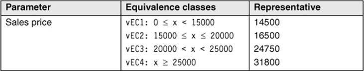
In section 2.2.2, the input values 14,500, 16,500, 24,750, 31,800 (see table 2-2) were chosen.

Every value is a representative for one of the four equivalence classes. It is assumed that test execution with input values like, for example, 13400, 17000, 22300, and 28900 does not lead to further insights and therefore does not find further failures. With this assumption, it is not necessary to execute those extra test cases. Note that tests with boundary values of the equivalence classes (for example, 15000) are discussed in section 5.1.2.

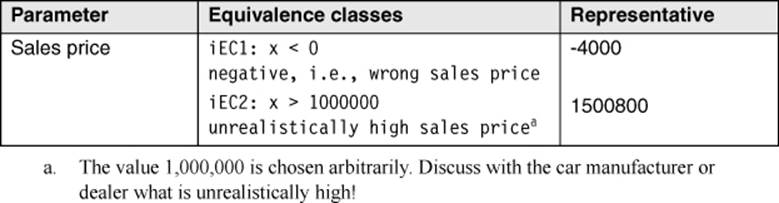
Equivalence classes with invalid values

Besides the correct input values, incorrect or invalid values must be tested. Equivalence classes for incorrect input values must be derived as well, and test cases with representatives of these classes must be executed. In the example we used earlier, there are the following two invalid equivalence classes⁴ (iEC).

Table 5–2
Invalid equivalence classes and representatives

Systematic development of the test cases

The following describes how to systematically derive the test cases. For every input data element that should be tested (e.g., function/method parameter at component tests or input screen field at system tests), the domain of all possible input values is determined. This domain is the equivalence class containing all valid or allowed input values. Following the specification, the program must correctly process these values. The values outside of this domain are seen as equivalence classes with invalid input values. For these values as well, it must be tested how the test object behaves.

Further partitioning of the equivalence classes

The next step is refining the equivalence classes. If the test object’s specification tells us that some elements of equivalence classes are processed differently, they should be assigned to a new (sub) equivalence class. The equivalence classes should be divided until each different requirement corresponds to an equivalence class. For every single equivalence class, a representative value should be chosen for a test case.

To complete the test cases, the tester must define the preconditions and the expected result for every test case.

Equivalence classes for output values

The same principle of dividing into equivalence classes can be used for the output data. However, identification of the individual test cases is more expensive because for every chosen output value, the corresponding input value combination causing this output must be determined. For the output values as well, the equivalence classes with incorrect values must not be left out.

Partitioning into equivalence classes and selecting the representatives should be done carefully. The probability of failure detection is highly dependent upon the quality of the partitioning as well as which test cases are executed. Usually, it is not trivial to produce the equivalence classes from the specification or from other documents.

Boundaries of the equivalence classes

The best test values are certainly those verifying the boundaries of the equivalence classes. There are often misunderstandings or inaccuracies in the requirements at these spots because our natural language is not precise enough to accurately define the limits of the equivalence classes. The colloquial phrase ... less than $15000 ... within the requirements may mean that the value 15000 is inside (EC: x <= 15000) or outside of the equivalence class (EC: x < 15000). An additional test case with x = 15000 may detect a misinterpretation and therefore failure. Section 5.1.2discusses the analysis of the boundary values for equivalence classes in detail.

Example: Equivalence class construction for integer input values

To clarify the procedure for building equivalence classes, all possible equivalence classes for an integer input value shall be identified. The following equivalence classes result for the integer parameter extras of the function calculate_price()::

Table 5–3
Equivalence classes for integer input values

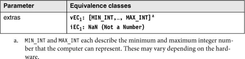
Notice that the domain is limited on a computer by the computer’s maximum and minimum values, contrary to plain mathematics. Using values outside the computer domain often leads to failures because such exceptions are not caught correctly.

The equivalence class for incorrect values is derived from the following consideration: Incorrect values are numbers that are greater or smaller than the range of the applicable interval or every nonnumeric value.⁵ If it is assumed that the program’s reaction on an incorrect value is always the same (e.g., an exception handling that delivers the error code NOT_VALID), then it is sufficient to map all possible incorrect values on one common equivalence class (named NaN for Not a Number here). Floating-point numbers are part of this equivalence class because it is expected that the program displays an error message to inputs such as 3.5. In this case, the equivalence class partitioning method does not require any further subdivision because the same reaction is expected for every wrong input. However, an experienced tester will always include a test case with a floating-point number in order to determine if the program rounds the number and then uses the corresponding integer number for its computation. The basis for this additional test case is thus experience-based testing (see section 5.3).

Because negative and positive values are usually handled differently, it is sensible to further partition the valid equivalence class (cEV1). Zero is also an input, which often leads to failure.

Table 5–4
Equivalence classes and representative values for integer inputs

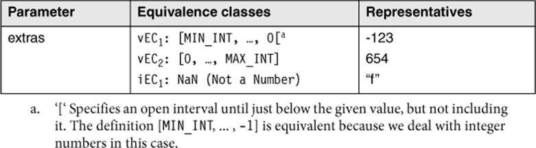
The representative was chosen relatively arbitrarily from the three equivalence classes. Additionally, we should test the boundary values (see section 5.1.2) of the corresponding equivalence classes: MIN_INT, -1, 0, MAX_INT. For the equivalence classes of the invalid values, no boundary values can be given.

Thus, using equivalence partitioning and including the boundary values for the integer parameter extras results in the following seven values to be tested:

{”f”, MIN_INT, -123, -1, 0, 654, MAX_INT}.

For each of these inputs, the predicted outputs or reactions of the test object must be defined, in order to decide after running the test if there was a failure.

Equivalence classes of inputs, which are no basic data types

For the integer input data of the example, it is very easy to determine equivalence classes and the corresponding representative test values. Besides the basic data types, data structures and sets of objects can also occur. It must then be decided in each case with which representative values to execute the test case.

Example for input values to be selected from a set

The following example should clarify this: A potential customer can be a working person, a student, a trainee, or a retired person. If the test object needs to react differently to each kind of customer, then every possibility must be verified with an additional test case. If there is no requirement for different reactions for each person type, then one test case may be sufficient.

If the test object is the component that calculates payment options (EasyFinance), then four different test cases must be provided. Financing will surely be calculated differently for the different customer groups. Details must be looked up in the requirements. Each calculation must be verified by a test to check the correctness of the calculations and to find failures.

For the test of the component that handles the online configuration of the car (VirtualShowRoom), it may be sufficient to choose only one representative for the customer, such as, for example, a working person. It is probably not relevant if a student or a retired person configures the car. The tester should, however, be aware that if she executes the test with the input working person only, she would not be able to tell anything about the correctness of the car configuration for any of the other person groups.

Hint for determining equivalence classes

The following hints can help determine equivalence classes:

§ For the inputs as well as for the outputs, identify the restrictions and conditions from the specification.

§ For every restriction or condition, partition into equivalence classes:

o If a continuous numerical domain is specified, then create one valid and two invalid equivalence classes.

o If a number of values should be entered, then create one valid (with all possible correct values) and two invalid equivalence classes (less and more than the correct number).

o If a set of values is specified where each value may possibly be treated differently, then create one valid equivalence class for each value of the set (containing exactly this one value) and one additional invalid equivalence class (containing all possible other values).

o If there is a condition that must be fulfilled, then create one valid and one invalid equivalence class to test the condition fulfilled and not fulfilled.

§ If there is any doubt that the values of one equivalence class are treated equally, the equivalence class should be divided further into subclasses.

Test Cases

Combination of the representatives

Usually, the test object has more than one input parameter. The equivalence class technique results in at least two equivalence classes (one valid and one invalid) for each of these parameters of the test object. Therefore, there are at least two representative values that must be used as test input for each parameter.

In order to specify a test case, you must assign each parameter an input value. For this purpose, it must be decided which of the available values should be combined to form test cases. To guarantee that all test object reactions (modeled by the equivalence class division) are triggered, you must combine the input values (i.e., the representatives of the corresponding equivalence classes), using the following rules:

Rules for test case design

§ The representative values of all valid equivalence classes should be combined to test cases, meaning that all possible combinations of valid equivalence classes will be covered. Any of those combinations builds a valid test case or a positive test case.

Separate test of the invalid value

§ The representative value of an invalid equivalence class shall be combined only with representatives of other valid equivalence classes. Thus, for every invalid equivalence class an additional negative test case shall be specified.

Restriction of the number of test cases

The number of valid test cases is the product of the number of valid equivalence classes per parameter. Because of this multiplicative combination, even a few parameters can generate hundreds of valid test cases. Since it is seldom possible to use that many test cases, more rules are necessary to reduce the number of valid test cases:

Rules for test case restriction

§ Combine the test cases and sort them by frequency of occurrence (typical usage profile). Prioritize the test cases in this order. That way only the relevant test cases (or combinations appearing often) are tested.

§ Test cases including boundary values or boundary value combinations are preferred.

§ Combine every representative of one equivalence class with every representative of the other equivalence classes (i.e., pairwise combinations⁶ instead of complete combinations).

§ Ensure that every representative of an equivalence class appears in at least one test case. This is a minimum criterion.

§ Representatives of invalid equivalence classes should not be combined with representatives of other invalid equivalence classes.

Test invalid values separately

The representatives of invalid equivalence classes are not combined. An invalid value should only be combined with valid ones because an incorrect parameter value normally triggers an exception handling. This is usually independent of values of other parameters. If a test case combines more than one incorrect value, defect masking may result and only one of the possible exceptions is actually triggered and tested. When a failure appears, it is not obvious which of the incorrect values has triggered the effect. This leads to extra time and cost for failure analysis.⁷

Example: Test of the DreamCar price calculation

In the following example, the function calculate_price() from the VSR-Subsystem DreamCar serves as test object (specified in section 3.2.3). We must test if the function calculates the correct total price from its input values. We assume that the inner structure of the function is unknown. Only the functional specification of the function and the external interface are known.

double calculate_price (
double baseprice, // base price of the vehicle
double specialprice, // special model addition
double extraprice, // price of the extras
int extras, // number of extras
double discount // dealer's discount
)

Step 1: Identifying the domain

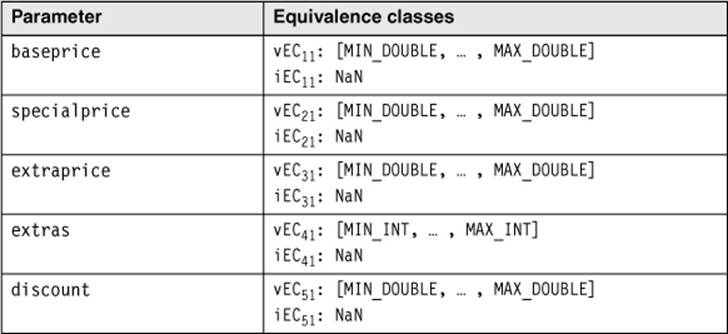
The equivalence class technique is used to derive the required test cases from the input parameters. First, we identify the domain for every input parameter. This results in equivalence classes for valid and invalid values for each parameter (see table 5-5).

With this technique, at least one valid and one invalid equivalence class per parameter has been derived exclusively from the interface specifications (test data generators work in a similar way; see section 7.1.2).

Table 5–5
Equivalence classes for integer input values

Step 2: Refine the equivalence classes based on the specification

In order to further subdivide these equivalence classes, information about the functionality of this method is needed. The functional specification delivers this information (see section 3.2.3). From this specification the following statements relevant for testing can be found:

§ Parameters 1 to 3 are prices (of cars). Prices are not negative. The specification does not define any price limits.

§ The value extras controls the discount for the supplementary equipment (10% if extras ≥ 3 and 15% if extras ≥ 5). The parameter extras defines the number of chosen parts of supplementary equipment and therefore it cannot be negative.⁸ The specification does not define an upper limit for the number.

§ The parameter discount denotes a general discount and is given as a percentage between 0 and 100. Because the specification text defines the limits for the discount for supplementary equipment as a percentage, the tester can assume that this parameter is entered as a percentage as well. Consultation with the client will otherwise clarify this matter.

These considerations are based not only on the functional specification. Rather, the analysis uncovers some “holes” in the specification. The tester fills these holes by making plausible assumptions based on application domain or general knowledge and her testing experience or by asking colleagues (testers or developers). If there is any doubt, consultation with the client is useful. The equivalence classes already defined before can be refined (partitioned into subclasses) during this analysis. The more detailed the equivalence classes are, the more precise the test. The class partition is complete when all conditions in the specification as well as conditions from the tester’s knowledge are incorporated.

Table 5–6
Further partitioning of the equivalence classes of the parameter of the function Calculate_price() with representatives

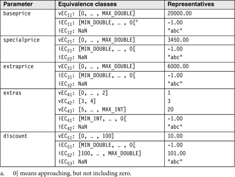
The result: Altogether, 18 equivalence classes are produced, 7 for correct/valid parameter values and 11 for incorrect/invalid ones.

Step 3: Select representatives

To get input data, one representative value must be chosen for every equivalence class. According to equivalence class theory, any value of an equivalence class can be used. In practice, perfect decomposition is seldom done. Due to an absence of detailed information, lack of time, or just lack of motivation, the decomposition is aborted at a certain level. Several equivalence classes might even (incorrectly) overlap.⁹ Therefore, one must remember that there could be values inside an equivalence class where the test object could react differently. Usage frequencies of different values may also be important.

Hence, in the example, the values for the valid equivalence classes are selected to represent plausible values and values that will probably often appear in practice. For invalid equivalence classes, possible values with low complexity are chosen. The selected values are shown in table 5-6.

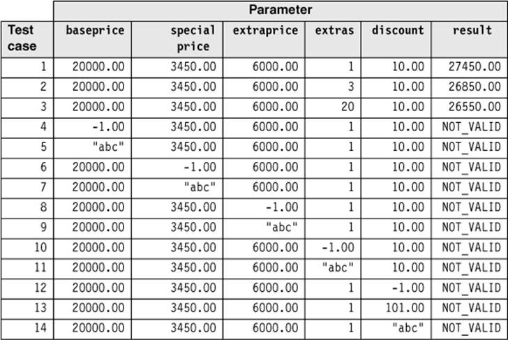
Step 4: Combine the test cases

The next step is to combine the values to test cases. Using the previously given rules, we get 1 × 1 × 1 × 3 × 1 = 3 valid test cases (by combining the representatives of the valid equivalence classes) and 2 + 2 + 2 + 2 + 3 = 11 negative test cases (by separately testing representatives of every invalid class). In total, 14 test cases result from the 18 equivalence classes (table 5-7).

Table 5–7
Further partitioning of the equivalence classes of the parameter test cases of the function Calculate_price()

For the valid equivalence classes, the same representative values were used to ensure that only the variance of one parameter triggers the reaction of the test object.

Because four out of five parameters have only one valid equivalence class, only a few valid test cases result. There is no reason to reduce the number of test cases any further.

After the test inputs have been chosen, the expected outcome must be identified for every test case. For the negative tests this is easy: The expected result is the corresponding error code or message. For the valid test cases, the expected outcome must be calculated (for example, by using a spreadsheet).

Definition of Test Exit Criteria

A test exit criterion for the test by equivalence class partitioning can be defined as the percentage of executed equivalence classes with respect to the total number of specified equivalence classes:

EC-coverage = (number of tested EC/total number of EC) × 100%

In the example, 18 equivalence classes have been defined, but only 15 have been executed in the chosen test cases. Then the equivalence class coverage is 83%.

EC-coverage = (15/18) × 100% = 83.33%

Example: Equivalence class coverage

All 18 equivalence classes are contained with at least one representative each in these 14 test cases (table 5-7). Thus, executing all 14 test cases achieves 100% equivalence class coverage. If the last three test cases are left out, for example due to time limitations (i.e., only 11 instead of 14 test cases are executed), all three invalid equivalence classes for the parameter discount are not tested and the coverage will be 15/18 (for example, 83.33%).

Degree of coverage defines test comprehensiveness

The more thoroughly a test object should be tested, the higher you should plan the intended coverage. Before test execution, the predefined coverage serves as a criterion for deciding when the testing is sufficient, and after test execution, it serves as verification if the required test intensity has been achieved.

If, in the previous example, the intended coverage for equivalence classes is defined as 80%, then this can be achieved with only 14 of the 18 tests. The test using equivalence class partitioning can be finished after 14 test cases. Thus, test coverage is a measurable criterion for ending testing.

The previous example also shows how critical it is to identify the equivalence classes. If the equivalence classes have not been identified completely, then fewer representative values will be chosen for designing test cases, and fewer test cases will result. A high coverage is achieved, but it has been calculated based on an incorrect total number of equivalence classes. The supposed good result does not reflect the actual intensity of the testing. Test case identification using equivalence class partitioning is only as good as the analysis it is based on.

The Value of the Technique

Equivalence class partitioning is a systematic technique. It contributes to a test where specified conditions and restrictions are not overlooked. The technique also reduces the amount of unnecessary test cases. Unnecessary test cases are the ones that have data from the same equivalence classes and therefore result in equal behavior of the test object.

Equivalence classes cannot be determined only for inputs and outputs of methods and functions. They can also be prepared for internal values and states, time-dependent values (for example, before or after an event), and interface parameters. The method can thus be used in any test level.

However, only single input or output conditions are considered. Possible dependencies or interactions between conditions are ignored. If they are considered, this is very expensive, but it can be done through further partitioning of the equivalence classes and by specifying appropriate combinations. This kind of combination testing is also called domain analysis.

However, in combination with fault-oriented techniques, like boundary value analysis, equivalence class partitioning is a powerful technique.

5.1.2 Boundary Value Analysis

A reasonable extension

→Boundary value analysis delivers a very reasonable addition to the test cases that have been identified by equivalence class partitioning. Faults often appear at the boundaries of equivalence classes. This happens because boundaries are often not defined clearly or are misunderstood. A test with boundary values usually discovers failures. The technique can be applied only if the set of data in one equivalence class is ordered and has identifiable boundaries.

Boundary value analysis checks the borders of the equivalence classes. On every border, the exact boundary value and both nearest adjacent values (inside and outside the equivalence class) are tested. The minimal possible increment in both directions should be used. For floating-point data, this can be the defined tolerance. Therefore, three test cases result from every boundary. If the upper boundary of one equivalence class equals the lower boundary of the adjacent equivalence class, then the respective test cases coincide as well.

In many cases there does not exist a “real” boundary value because the boundary value belongs to an equivalence class. In such cases, it can be sufficient to test the boundary with two values: one value that is just inside the equivalence class and another value that is just outside the equivalence class.

Example: Boundary values for discount

For computing the discount on the sales price (table 5-1), four valid equivalence classes were determined and corresponding values chosen for testing the classes. Equivalence classes 3 and 4 are specified with vEC3: 20000 < x ≤ 25000 and vEC4: x ≥ 25000. For testing the common boundary of the two equivalence classes (25000), the values 24999 and 25000 are chosen (to simplify the situation, it is assumed that only whole dollars are possible). The value 24999 lies in vEC3 and is the largest possible value in that equivalence class. The value 25000 is the least possible value in vEC4. The values 24998 and 25001 do not give any more information because they are further inside their corresponding equivalence classes. Thus, when are the values 24999 and 25000 sufficient and when should we additionally use the value 25001?

Two or three tests

It can help to look at the implementation. The program will probably contain the →instruction if (x < 25000)....¹⁰ Which test cases could find a wrong implementation of this condition? The test values 24999, 25000, and 25001 generate the truth-values true, false, and false for the IF statement and the corresponding program parts are executed. Test value 25001 does not seem to add any value because test value 25000 already generates the truth-value false (and thus the change to the neighbor equivalence class). Wrong implementation of the statement if (x ≤ 25000) leads to the truth-values true, true, and false. Even here, a test with the value 25001 does not lead to any new results and can thus be omitted, because the test with value 25000 will lead to a failure and thus find the fault. Only a totally wrong implementation stating, for example, if (x <> 25000) and the truth-values true, false, and true can be found with test case value 25001. The values 24999 and 25000 deliver the expected results, that is, the same ones as with the correct implementation.

Hint

Wrong implementation of the instruction in if (x > 25000) with false, false, and true and in if (x ≥ 25000) with false, true, and true results in two or three differences between actual and expected result and can be found by test cases with the values 24999 and 25000.

To illustrate the facts, table 5-8 shows the different conditions and the truth-values of the corresponding boundary values.

Table 5–8
Table with three boundary values to test the condition

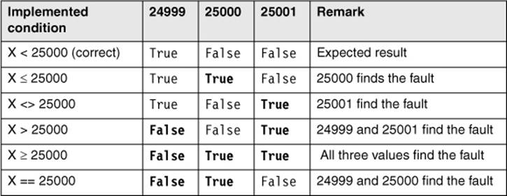
It should be decided when a test with only two values is considered enough or when it is beneficial to test the boundary with three values. The wrong query in the example program, implemented as if (x <> 25000), can be found in a code review because it does not check the boundary of a value area if (x < 25000) but instead checks whether two values are unequal. However, this fault can easily be overlooked. Only with a boundary value test with three values can all possible wrong implementations of boundary conditions be found.

Example: Integer input

A test involving an integer input value (see section 5.1.1) produces 5 new test cases, giving us a total of 12 test cases with the following input values:

{"f",
MIN_INT-1, MIN_INT, MIN_INT+1,
-123,
-1, 0, 1,
654,
MAX_INT-1, MAX_INT, MAX_INT+1}

The test case with the input value -1 tests the maximum value of the equivalence class EC1: [MIN_INT, ... 0[. This test case also verifies the smallest deviation from the lower boundary (0) of the equivalence class EC2: [0, ..., MAX_INT]. Seen from EC2, the value lies outside this equivalence class. Note that values above the uppermost boundary as well as beneath the lowermost boundary cannot always be entered due to technical reasons.

Only test values for the input variable are given in this example. To complete the test cases for each of the 12 values, the expected behavior of the test object and the expected outcome must be specified using the test oracle. Additionally, the applicable pre- and postconditions are necessary.

Is the test cost justified?

Here too we have to decide if the test cost is justified, and every boundary with the adjacent values must be tested with extra test cases. Test cases with values of equivalence classes that do not verify any boundary can be dropped. In the example, these are the test cases with the input values -123 and 654. It is assumed that test cases with values in the middle of an equivalence class do not deliver any new insight. This is because the maximum and the minimum values of the equivalence class are already chosen in some test cases. In the example these values are MIN_INT+1, 1, and MAX_INT-1.

Boundaries do not exist for sets

For the example with the input data element customer given earlier, no boundaries for the input domain can be found. The input data type is discrete, that is, a set of the four elements (working person, student, trainee, and retired person). Boundaries cannot be identified here. A possible order by age cannot be defined clearly.

Of course, boundary value analysis can also be applied for output equivalence classes.

Test Cases

Analogous to the test case determination in equivalence class partition, the valid boundaries inside an equivalence class may be combined as test cases. The invalid boundaries must be verified separately and cannot be combined with other invalid boundaries.

As described in the previous example, values from the middle of an equivalence class are, in principle, not necessary if the two boundary values in an equivalence class are used for test cases.

Example: Boundary values for calculate_price()

Table 5-9 lists the boundary values for the valid equivalence classes for verification of the function calculate_price().

Table 5–9
Boundaries of the parameters of the function calculate_price()

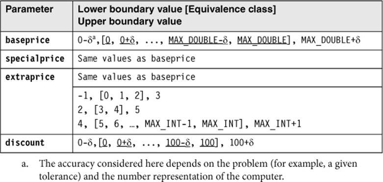
Considering only those boundaries that can be found inside equivalence classes, we get 4 + 4 + 4 + 9 + 4 = 25 boundary-based values. Of these, two (extras: 1, 3) are already tested in the original equivalence class partitioning in the example before (test cases 1 and 2 in table 5-7). Thus, the following 23 boundary values must be used for new test cases:

baseprice: 0.00, 0.01¹¹, MAX_DOUBLE-0.01, MAX_DOUBLE
specialprice: 0.00, 0.01, MAX_DOUBLE-0.01, MAX_DOUBLE
extraprice: 0.00, 0.01, MAX_DOUBLE-0.01, MAX_DOUBLE
extras: 0, 2, 4, 5, 6, MAX_INT-1, MAX_INT
discount: 0.00, 0.01, 99.99, 100.00

As all values are valid boundaries, they can be combined into test cases (table 5-10).

The expected results of a boundary value test are often not clearly visible from the specification. The experienced tester must then define reasonable expected results for her test cases:

§ Test case 15 verifies all valid lower boundaries of equivalence classes of the parameters of calculate_price(). The test case doesn’t seem to be very realistic.¹² This is because of the imprecise specification of the functionality, where no lower and upper boundaries are specified for the parameters (see below).¹³

§ Test case 16 is analogous to test case 15, but here we test the precision of the calculation.¹⁴

§ Test case 17 combines the next boundaries from table 5-9. The expected result is rather speculative with a discount of 99.99%. A look into the specification of the method calculate_price() shows that the prices are added. Thus, it makes sense to check the maximal values individually. Test cases 18 to 20 do this. For the other parameters, we use the values from test case 1 (table 5-7). Further sensible test cases result when the values of the other parameters are set to 0.00, in order to check if maximal values without further addition are handled correctly and without overflow.

§ Analogous to test cases 17 to 20, test cases for MAX_DOUBLE should be run.

§ For the still-not-tested boundary values (extras = 5, 6, MAX_INT-1, MAX_INT and discount = 100.00), more test cases are needed.

Boundary values outside the valid equivalence classes are not used here.

The example shows the detrimental effect of imprecise specifications on the test.¹⁵ If the tester communicates with the customer before determining the test cases, and the value ranges of the parameters can be specified more precisely, then the test will be less expensive. This is shown here.

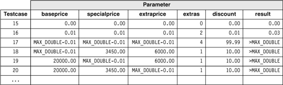
Table 5–10
Further test cases for the function calculate_price()s

Early test planning—already during specification—pays off

The customer has given the following information:

§ The base price is between 10000 and 150000.

§ The extra price for a special model is between 800 and 3500.

§ There are a maximum of 25 possible extras, whose prices are between 50 and 750.

§ The dealer discount is maximum 25%.

After specifying the equivalence classes, the following valid boundary values result for the parameters:

baseprice: 10000.00, 10000.01, 149999.99, 150000.00
specialprice: 800.00, 800.01, 3499.99, 3500.00
extraprice: 50.00, 50.01, 18749.99, 18750.00¹⁶
extras: 0, 1, 2, 3, 4, 5, 6, 24, 25
discount: 0.00, 0.01, 24.99, 25.00

All these values may be freely combined to test cases. One test case is needed for each value outside the equivalence classes. The following values must be considered:

baseprice: 9999.99, 150000.01
specialprice: 799.99, 3500.01
extraprice: 49.99, 18750.01
extras: -1, 26
discount: -0.01, 25.01

Thus, we see that a more precise specification results in fewer test cases and clear prediction of the results.

Adding the boundary values for the machine (MAX_DOUBLE, MIN_DOUBLE, etc.) is a good idea. This will detect problems with hardware restrictions.

As discussed earlier, it must be decided if it is sufficient to test a boundary with two instead of three test data values. In the following hints, we assume that two test values are sufficient because there has been a code review and possible totally wrong value area checks have been found.

Hint for test case design by boundary analysis

§ For an input domain, the boundaries and the adjacent values outside the domain must be considered. Domain: [-1.0; +1.0], test data: -1.0, +1.0 and -1.001, +1.001.¹⁷

§ If an input file has a restricted number of data records (for example, between 1 and 100), the test values should be 1, 100 and 0, 101.

§ If the output domains serve as the basis, then this is the way to proceed: The output of the test object is an integer value between 500 and 1000. Test outputs that should be achieved: 500, 1000, 499, 1001. Indeed, it can be difficult to identify the respective input test data to achieve exactly the required outputs. Generating the invalid outputs may even be impossible, but you may find defects by thinking about it.

§ If the permitted number of output values is to be tested, proceed just as with the number of input values: If outputs of 1 to 4 data values are allowed, the test outputs to produce are 1, 4 as well as 0 and 5 data values.

§ For ordered sets, the first element and the last element are of special interest for the test.

§ If complex data structures are given as input or output (for instance, an empty list or zero), tables can be considered as boundary values.

§ For numeric calculations, values that are close together, as well as values that are far apart, should be taken into consideration as boundary values.

§ For invalid equivalence classes, boundary value analysis is only useful when different exception handling for the test object is expected, depending on an equivalence class boundary.

§ Additionally, extremely large data structures, lists, tables, etc. should be chosen. For example, you should exceed buffer, file, or data storage boundaries, in order to check the behavior of the test object in extreme cases.

§ For lists and tables, empty and full lists and the first and last elements are of interest because they often show failures due to incorrect programming (Off-by-one problem).

Definition of the Test Exit Criteria

Analogous to the test completion criterion for equivalence class partition, an intended coverage of the boundary values (BVs) can also be predefined and calculated after execution of the tests.

BV-Coverage = (number of tested BV / total number of BV) × 100%

Notice that the boundary values, as well as the corresponding adjacent values above and below the boundary, must be counted. However, only differing values are used for the calculation. Overlapping values of adjacent equivalence classes are counted as only one boundary value because only one test case with the respective input value is used.

The Value of the Technique

In combination with equivalence class partitioning

Boundary value analysis should be used together with equivalence class partitioning because faults can be found more often at the boundaries of the equivalence classes than far inside the classes. It makes sense to combine both techniques, but the technique still allows enough freedom in selecting the concrete test data.

The technique requires a lot of creativity to define appropriate test data at the boundaries. This aspect is often ignored because the technique appears to be very easy, even though determining the relevant boundaries is not at all trivial.

5.1.3 State Transition Testing

Consider history

In many systems, not only the current input but also the history of execution or events or inputs influences computation of the outputs and how the system will behave. History of system execution needs to be taken into account. To illustrate the dependence on history, →state diagrams are used. They are the basis for designing the test (→state transition testing).

The system or test object starts from an initial state and can then comes into different states. Events trigger state changes or transitions. An event may be a function invocation. State transitions can involve actions. Besides the initial state, the other special state is the end state. →Finite state machines, state diagrams, and state transition tables model this behavior.

Definition of a finite state machine

A finite state machine is formally defined as follows: An abstract machine for which the number of states and input symbols are both finite and fixed. A finite state machine consists of states (nodes), transitions (links), inputs (link weights), and outputs (link weights). There are a finite number of internal configurations, called states. The state of a system implicitly contains the information that has resulted from the earlier inputs and that is necessary to find the reaction of the system to new inputs.

Example: Stack

Figure 5-3 shows the popular example of a stack. The stack—for example, a dish stack in a heating device—can be in three different states: empty, filled, and full.

The stack is “empty” after initializing where the maximum height (Max) is defined (current height = 0). By adding an element to the stack (calling the function push), the state changes to “filled” and the current height is incremented. In this state further elements can be added (push, increment height) as well as withdrawn (call of the function pop, decrement height). The uppermost element can also be displayed (call of the function top, height unchanged). Displaying does not alter the stack itself and therefore does not remove any element. If the current height is one less than the maximum (height = Max – 1) and one element is added to the stack (push), then the state of the stack changes from “filled” to “full.” No further element can be added. The condition (Max –1) is described as the guard for the transition between the initial and the resulting state. Appropriate guards are illustrated in figure 5-3. If one element is removed (pop) from a stack in the “full” state, the state is changed back from “full” to “filled.” A transition from “filled” to “empty” happens only if the stack consists of just one element, which is removed (pop). The stack can only be deleted in the “empty” state.

Figure 5–3
State diagram of a stack

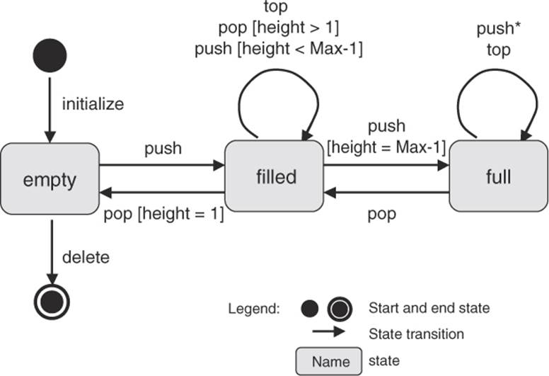
Depending upon the specification, you can define which functions (push, pop, top, etc.) can be called for which state of the stack. You must still clarify what happens when an element is added to a “full” stack (push*). The function must work differently from the case of a just–“filled” stack. Thus, the functions must behave differently depending on the state of the stack. The state of the test object is a decisive element and must be taken into account when testing.¹⁸

A possible concrete test case

Here is a possible test case with pre- and postconditions for a stack that may store text strings:

Further functions of the stack (showing the current level, showing the maximum level, enquiry if the stack is empty, etc.) are not considered in this example because they do not change the state of the stack.

The test object in state transition testing

In state transition testing, the test object can be a complete system with different system states as well as a class in an object-oriented system with different states. Whenever the input history leads to differing behavior, a state transition test must be applied.

Further test cases for the stack example

Different levels of test intensity can be defined for a state transition test. A minimum requirement is to get to all possible states. In the stack example, these states are empty, filled, and full.¹⁹ With an assumed maximum height of 4, all three states are reached after calling the following functions:

Test case 1:²⁰ initialize [empty], push [filled], push, push, push [full].

Yet, even not all the functions of the stack have been called in this test.

Another requirement for the test is to invoke all functions. With the same stack as before, the following sequence of function calls is sufficient for compliance with this requirement:

Test case 2: initialize [empty], push [filled], top, pop [empty], delete.

However, in this sequence, not all the states have been reached.

Test criteria

A state transition test should execute all specified functions of a state at least once. Compliance between the specified and the actual behavior of the test object can thus be checked.

Design a transition tree

To identify the necessary test cases, the finite state machine is transformed into a so-called transition tree, which includes certain sequences of transitions ([Chow 78]). The cyclic state transition diagram with potentially infinite sequences of states changes to a transition tree, which corresponds to a representative number of states without cycles. With this translation, all states must be reached and all transitions of the transition diagram must appear.

The transition tree is built from a transition diagram this way:

1. The initial or start state is the root of the tree.

2. For every possible transition from the initial state to a following state in the state transition diagram, the transition tree receives a branch from its root to a node, representing this next state.

3. The process for step 2 is repeated for every leaf in the tree (every newly added node) until one of the following two end conditions is fulfilled:

o The corresponding state is already included in the tree on the way from the root to the node. This end condition corresponds to one execution of a cycle in the transition diagram.

o The corresponding state is a final state and therefore has no further transitions to be considered.

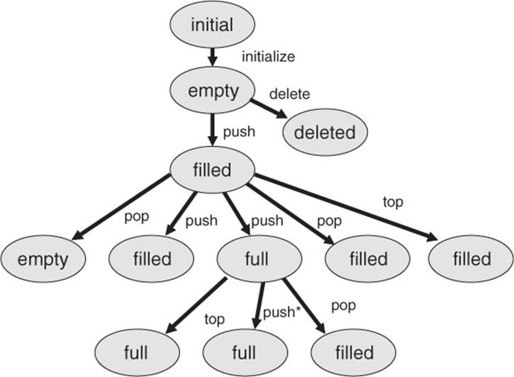
For the stack, the resulting transition tree is shown in figure 5-4.

Eight different paths can be recognized from the root to each of the end nodes (leaves). Each path represents a test case, that is, a sequence of function calls. Thereby, every state is reached at least once, and every possible function is called in each state according to the specification of the state transition diagram.

However, the transition tree doesn’t show the appropriate guards, but they need to be taken care of when test cases are designed.

In test case 1 (shown previously), the maximum assumed stack height is four and the guard condition for the transition from the filled to the full state when push is called is max. height (4) – 1 = 3. Three push calls are therefore necessary to pass from filled to full in the transition tree. In addition, another first push call serves to change the state from empty to filled. If no guard conditions are set in a transition tree (as in figures 5-4 and 5-5), it looks like a single push call is sufficient to move from the filled to the full state.

Figure 5–4
Transition tree for the stack example

The transition tree shown in figure 5-4 includes all possible call sequences resulting from the state model shown in figure 5-3. In addition, the reaction of the state machine for wrong usage must be checked, which means that functions are called in states in which they are not supposed to be called. Here again the remark that push needs to work differently depends on the state. If push is called in the “full” state, it cannot add an element to the stack but must leave it unchanged. A message may result, but this is not the same as a fault.

Incorrect use of functions

It is a violation of the specification if functions are called in states where they should not be used (e.g., to delete the stack while in the “full” state). A robustness test must be executed to check how the test object works when used incorrectly. It should be tested to see whether unexpected transitions appear. The test can be seen as an analogy to the test of unexpected input values.

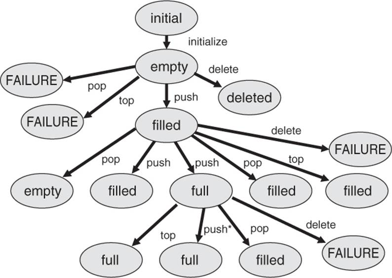
The transition tree should be extended by adding a branch for every function from every node. This means that from every state, all the functions should be executed or at least an attempt should be made to execute them (see figure 5-5).

Producing an extended transition tree can help to find gaps in the specifications.

Here, for example, the pop and top calls that weren’t present in the state diagram in figure 5-3 (i.e., that weren’t specified) have been added to the state “empty.” It definitely makes sense to define which reactions to expect when trying pop and top calls for an empty stack. A reasonable reaction would be, for example, an error message.

Figure 5–5
Transition tree for the test for robustness

State transition testing is also a good technique for system testing when testing the graphical user interface (GUI) of the test object: The GUI usually consists of a set of screens and dialog boxes; between those, the user can switch back and forth (via menu choices, an OK button, etc.). If screens and user controls are seen as states and input reactions as state transitions, then the GUI can be modeled with a state diagram. Appropriate test cases and test coverage can be identified by the state transition testing technique described earlier.

Example: Test of DreamCar-GUI

When testing the DreamCar GUI, it may look like this:

Figure 5–6
GUI navigation as state graph

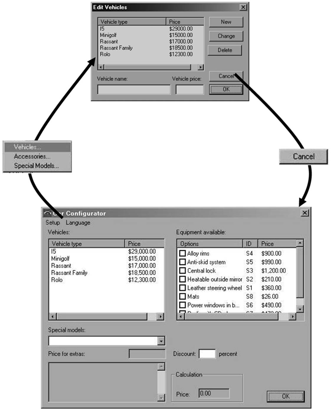
The test starts at the DreamCar main screen (state 1). The action²¹ “Setup vehicles” triggers the transition into the dialog “Edit vehicle” (state 2). The action “Cancel” ends this dialog and the application returns to state 1. Inside a state we can then use “local” tests, which do not change the state. These tests then verify the built-in functionality of the accessed screen. Navigation through arbitrarily complex chains of dialogs can then be modeled after this action. The state diagram of the GUI ensures that all dialogs are included and verified in the test.

Test Cases

To completely define a state-based test case, the following information is necessary:

§ The initial state of the test object (component or system)

§ The inputs to the test object

§ The expected outcome or expected behavior

§ The expected final state

Further, for each expected state transition of the test case, the following aspects must be defined:

§ The state before the transition

§ The initiating event that triggers the transition

§ The expected reaction triggered by the transition

§ The next expected state

It is not always easy to identify the states of a test object. Often, the state is not defined by a single variable but is rather the result from a constellation of values of several variables. These variables may be deeply hidden in the test object. Thus, the verification and evaluation of each test case can be very expensive.

Hint

§ Evaluate the state transition diagram from a testing point of view when writing the specification. If there are a high number of states and transitions, indicate the higher test effort and push for simplification if possible.

§ Check the specification, as well, to make sure the different states are easy to identify and that they are not the result of a multiple combination of values of different variables.

§ Check that the state variables are easy to display from the outside. It is a good idea to include functions that set, reset, and read the state for use during testing.

Definition of the Test Exit Criteria

Criteria for test intensity and for exiting can also be defined for state transition testing:

§ Every state has been reached at least once.

§ Every transition has been executed at least once.

§ Every transition violating the specification has been checked.

Percentages can be defined using the proportion of test requirements that were actually executed to possible ones, similar to the earlier described coverage measures.

Higher-level criteria

For highly critical applications, more stringent state transition test completion criteria can be defined:

§ All combination of transitions

§ All transitions in any order with all possible states, including multiple executions in a row

But, achieving sufficient coverage is often not possible due to the large number of necessary test cases. Therefore, it is reasonable to set a limit to the number of combinations or sequences that must be verified.

The Value of the Technique

State transition testing should be applied where states are important and where the functionality is influenced by the current state of the test object. The other testing techniques that have been introduced do not support these aspects because they do not account for the different behavior of the functions in different states.

Especially useful for test of object-oriented systems

In object-oriented systems, objects can have different states. The corresponding methods to manipulate the objects must then react according to what state they are in. State transition testing is therefore more important for object-oriented testing because it takes into account this special aspect of object orientation.

5.1.4 Logic-Based Techniques (Cause-Effect Graphing and Decision Table Technique, Pairwise Testing)

The previously introduced techniques look at the different input data independently. The input values are each considered separately for generating test cases. Dependencies among the different inputs and their effects on the outputs are not explicitly considered for test case design.

Cause-effect graphing

[Myers 79] describes a technique that uses the dependencies for identification of the test cases. It is known as →cause-effect graphing. The logical relationships between the causes and their effects in a component or a system are displayed in a so-called cause-effect graph. The precondition is that it is possible to find the causes and effects from the specification. Every cause is described as a condition that consists of input values (or combinations thereof). The conditions are connected with logical operators (e.g., AND, OR, NOT). The condition, and thus its cause, can be true or false. Effects are treated similarly and described in the graph (see figure 5-7).

Example: Cause-effect graph for an ATM

In the following example, we’ll use the act of withdrawing money at an automated teller machine (ATM) to illustrate how to prepare a cause-effect graph. In order to get money from the machine, the following conditions must be fulfilled:²²

§ The bank card is valid.

§ The PIN is entered correctly.

§ The maximum number of PIN inputs is three.

§ There is money in the machine and in the account.

The following actions are possible at the machine:

§ Reject card.

§ Ask for another PIN input.

§ “Eat” the card.

§ Ask for an other amount.

§ Pay the requested amount of money.

Figure 5-7 shows the cause-effect graph of the example.

Figure 5–7
Cause-effect graph of the ATM

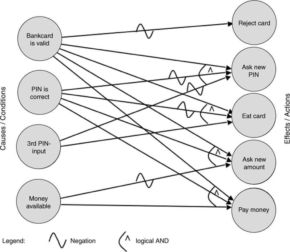
The graph makes clear which conditions must be combined in order to achieve the corresponding effects.

The graph must be transformed into a →decision table from which the test cases can be derived. The steps to transform a graph into a table are as follows:

1. Choose an effect.

2. Looking in the graph, find combinations of causes that have this effect and combinations that do not have this effect.

3. Add one column into the table for every one of these cause-effect combinations. Include the caused states of the remaining effects.

4. Check to see if decision table entries occur several times, and if they do, delete them.

Test with decision tables

The objective for a test based on decision tables is that it executes “interesting” combinations of inputs—interesting in the sense that potential failures can be detected. Besides the causes and effects, intermediate results with their truth-values may be included in the decision table.

A decision table has two parts. In the upper half, the inputs (causes) are listed; the lower half contains the effects. Every column defines the test situations, i.e., the combination of conditions and the expected effects or outputs.

In the easiest case, every combination of causes leads to one test case. However, conditions may influence or exclude each other in such a way that not all combinations make sense. The fulfillment of every cause and effect is noted in the table with a “yes” or “no.” Each cause and effect should at least once have the values “yes” and “no” in the table.

Example: Decision table for an ATM

Because there are four conditions (from “bank card is valid” to “money available”), there are, theoretically, 16 (2⁴) possible combinations. However, not all dependencies are taken into account here. For example, if the bank card is invalid, the other conditions are not interesting because the machine should reject the card.

An optimized decision table does not contain all possible combinations, but the impossible or unnecessary combinations are not entered. The dependencies between the inputs and the results (actions, outputs) lead to the following optimized decision table, showing the result (table 5-11).

Table 5–11
Optimized decision table for the ATM

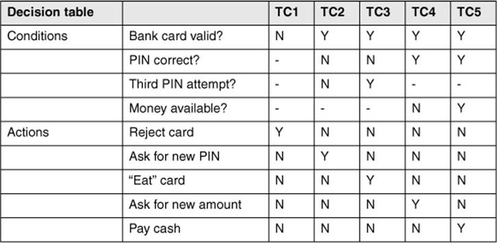
Every column of this table is to be interpreted as a test case. From the table, the necessary input conditions and expected actions can be found directly. Test case 5 shows the following condition: The money is delivered only if the card is valid, the PIN is correct after a maximum of three tries, and there is money available both in the machine and in the account.

This relatively small example shows how more conditions or dependencies can soon result in large and unwieldy graphs or tables.

From a decision table, a decision tree may be derived. The decision tree is analogous to the transition tree in state transition testing in how it’s used.

Every path from the root of the tree to a leaf corresponds to a test case. Every node on the way to a leaf contains a condition that determines the further path, depending on its truth-value.

Test Cases

Every column is a test case

In a decision table, the conditions and dependencies for the inputs, the corresponding predicted outputs, and the results for this combination of inputs can be read directly from every column to form a test case. The table defines logical test cases. They must be fed with concrete data values in order to be executed, and necessary preconditions and postconditions must be defined.

Definition of the Test Exit Criteria

Simple criteria for test exit

As with the previous methods, criteria for test completion can be defined relatively easily. A minimum requirement is to execute every column in the decision table by at least one test case. This verifies all sensible combinations of conditions and their corresponding effects.

The Value of the Technique

The systematic and very formal approach in defining a decision table with all possible combinations may show combinations that are not included when other test case design techniques are used. However, errors can result from optimization of the decision table, such as, for example, when the input and condition combinations to be considered are (erroneously) left out.

As mentioned, the graph and the table may grow quickly and lose readability when the number of conditions and dependent actions increases. Without adequate support by tools, the technique is then very difficult.

Pairwise Combination Testing

This test design technique can be used when interactions between different parameters are unknown. This is the opposite of cause-effect graphing, which is designed to cover explicitly known dependencies. Pairwise combination testing has the objective of finding destructive interaction between presumably independent parameters (or parameters for which the specification does not include dependencies).

The technique starts from the equivalence class table. For every equivalence class,²³ a representative value is chosen. Then, every representative for one class is combined with every representative for every other class (taking into account only pairs of combinations, not higher-level combinations).

After installation of the DreamCar subsystem, three parameters must be set: the operating system (Mac, Linux, or Windows), the language (German, Norwegian, English), and the screen size (small, large). If all combinations were chosen to test this, 3 × 3 × 2 = 18 test cases would result. However, choosing pair wise combinations, we need only 9 test cases. Table 5-12 shows a possible solution.

Table 5–12
Pairwise combinations

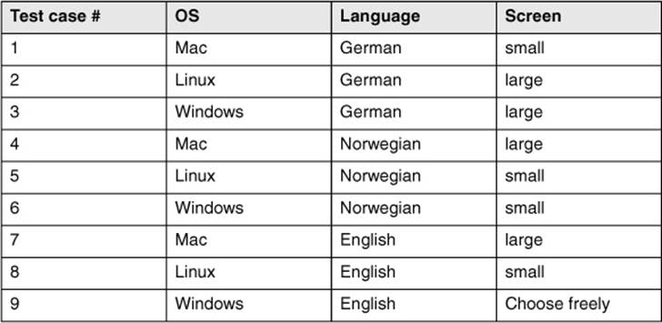
The solution shows that each operating system occurs with every possible language and every possible screen size. Every language also occurs with every possible screen size and with every possible operating system. Finally, every possible screen size occurs with every language and with every operating system. But not every possible triple combination (such as Mac, English, small) occurs in the test. Test case 9 is special: The combination of Windows and English is necessary, but any combinations with the screen size have already been covered in other test cases. Thus, the screen size can be freely chosen; for example, the most often occurring one can be used.

Pairwise combination tests will find any destructive interaction between supposedly independent parameters (provided the representative values chosen do this). Higher-level interactions will not necessarily be discovered.

The technique is not easy to apply manually, but tools are available [URL: pairwise].

The technique can be extended to cover higher levels of interaction.

5.1.5 Use-Case-Based Testing

UML is widely used

With the increasing use of object-oriented methods for software development, the Unified Modeling Language (UML) ([URL: UML]) is used ever more frequently in practice. UML defines more than 10 graphical notations that can be used in all kinds of software development, not only object-oriented.

→Use case testing

There are many research projects and approaches to directly derive test cases from UML diagrams and to generate these tests more or less automatically. One current issue is model-based testing.²⁴

Requirements identification

Requirements may be described as →use cases or business cases. They may be given as diagrams. The diagrams help define requirements on a relatively abstract level by describing typical user-system interactions. Testers may utilize use cases to derive test cases.

Figure 5-8 shows a use case diagram for part of the dialog with an ATM for withdrawing money.

The individual use cases in this example are “Get money,” “PIN query,” and “Eat card.” Relationships between use cases may be “include” and “extend.” “Include” conditions are always used, and “extend” connections can lead to extensions of a use case under certain conditions at a certain point (extension point). Thus, the “extend” conditions are not always executed; there are alternatives.

Figure 5–8
Use case diagram for ATM

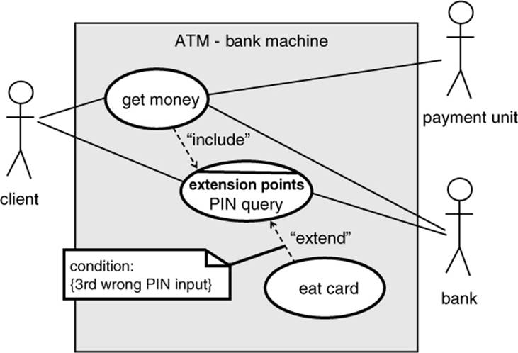
Showing an external view

Use case diagrams mainly serve to show the external view of a system from the viewpoint of the user or to show the relation to neighboring systems. Such external connections are shown as lines to actors (for example, the man symbol in the figure). There are further elements in a use case diagram that are included in this discussion.

Pre- and postconditions

For every use case, certain preconditions must be fulfilled to enable its execution. A precondition for getting money at the ATM is, for example, that the bank card is valid. After a use case is executed, there are postconditions. For example, after successfully entering the correct PIN, it is possible to get money. However, first the amount must be entered, and it must be confirmed that the money is available. Pre- and postconditions are also applicable for the flow of use cases in a diagram, that is, the path through the diagram.

Useful for system and acceptance testing

Use cases and use case diagrams serve as the basis for determining test cases in use-case-based testing. As the external view is modeled, the technique is very useful for both system testing and acceptance testing. If the diagrams are used to model the interactions between different subsystems, test cases can also be derived for integration testing.

Typical system use is tested

The diagrams show the “normal,” “typical,” and “probable” flows and often their alternatives. Thus, the use-case-based test checks typical use of a system. It is especially important for acceptance of a system that it runs as stable as possible in “normal” use. Thus, use-case-based testing is highly relevant for the customer and user and therefore for the developer and tester as well.

Test Cases

Every use case has a purpose and shall achieve a certain result. Events may occur that lead to further alternatives or activities. After the execution, there are postconditions. All of the following information is necessary for designing test cases and is thus available:

§ Start situation and preconditions

§ Possibly other conditions

§ Expected results

§ Postconditions

However, the concrete input data and results for the individual test cases cannot be derived directly from the use cases. The individual input and output data must be chosen. Additionally, each alternative contained in the diagram (“extend” relation) must be covered by a test case. The techniques for designing test cases on the basis of use cases may be combined with other specification-based test design techniques.

Definition of the Test Exit Criteria

A possible criterion is that every use case or every possible sequence of use cases in the diagram is tested at least once by a test case. Since alternatives and extensions are use cases too, this criterion also requires their execution.

The Value of the Technique

Use-case-based testing is very useful for testing typical user-system interactions. Thus, it is best to apply it in acceptance testing and in system testing. Additionally, test specification tools are available to support this approach (section 7.1.4). “Expected” exceptions and special treatment of cases can be shown in the diagram and included in the test cases, such as, for example, entering a wrong PIN three times (see figure 5-8). However, no systematic method exists to determine further test cases for testing facts that are not shown in the use case diagram. The other test techniques, such as boundary value analysis, are helpful for this.

Excursion

This section definitely did not describe all black box test design techniques. We’ll briefly describe a few more techniques here to offer some tips about their selection. Further techniques can be found in [Myers 79], [Beizer 90], [Beizer 95], and [Pol 98].

Syntax test

→Syntax testing describes a technique for identifying test cases that can be applied if a formal specification of the syntax of the inputs is available. Syntax testing would be used for testing interpreters of command languages, compilers, and protocol analyzers, for example. The syntax definition is used to specify test cases that cover both the compliance to and violation of the syntax rules for the inputs [Beizer 90].

Random test

→Random testing generates values for the test cases by random selection. If a statistical distribution of the input values is given (e.g., normal distribution), then it should be used for the selection of test values. This ensures that the test cases are preferably close to reality, making it possible to use statistical models for predicting or certifying system reliability [IEEE 982], [Musa 87].

Smoke test

The term smoke test is often used in software testing. A smoke test is commonly understood as a “quick and dirty” test that is primarily aimed at verifying the minimum reliability of the test object. The test is concentrated on the main functions of the test object. The output of the test is not evaluated in detail. It is checked only if the test object crashes or seriously misbehaves. A test oracle is not used, which contributes to making this test inexpensive and easy. The term smoke test is derived from testing old-fashioned electrical circuits because short circuits lead to smoke rising. A smoke test is often used to decide if the test object is mature enough to proceed with further testing designed with the more comprehensive test techniques. Smoke tests can also be used for first and fast tests of software updates.

5.1.6 General Discussion of the Black Box Technique

Wrong specification is not detected

The basis of all black box techniques is the requirements or specifications of the system or its components and how they collaborate. Black box testing will not be able to find problems where the implementation is based on incorrect requirements or a faulty design specification because there will be no deviation between the faulty specification or design and the observed results. The test object will execute as the requirements or specifications require, even when they are wrong. If the tester is critical toward the requirements or specifications and uses “common sense”, she may find wrong requirements during test design.

Otherwise, to find inconsistencies and problems in the specifications, reviews must be used (section 4.1.2).

Functionality that’s not required is not detected

In addition, black box testing cannot reveal extra functionality that exceeds the specifications. (Such extra functionality is often the cause of security problems.) Sometimes additional functions are neither specified nor required by the customer. Test cases that execute those additional functions are performed by pure chance if at all. The coverage criteria, which serve as conditions for test exit, are exclusively identified on the basis of the specifications or requirements. They are not based on unmentioned or assumed functions.

Verification of the functionality

The center of attention for all black box techniques is the verification of the functionality of the test object. It is indisputable that the highest priority is that the software work correctly. Thus, black box techniques should always be applied.

5.2 White Box Testing Techniques

Code-based testing techniques

The basis for white box techniques is the source code of the test object.

Therefore, these techniques are often called structure-based testing techniques because they are based on the structure (of the program). They are also called →code-based testing techniques. The source code must be available, and in certain cases, it must be possible to manipulate it, that is, to add code.

All code should be executed

The foundation of white box techniques is to execute every part of the code of the test object at least once. Flow-oriented test cases are identified, analyzing the program logic, and then they are executed. However, the expected results should be determined using the requirements or specifications, not the code. This is done in order to decide if execution resulted in a failure.

A white box technique can focus on, for example, the statements of the test object. The primary goal of the technique is then to achieve a previously defined coverage of the statements during testing, such as, for example, to execute as many statements of the program as possible.

These are the white box test case design techniques:

§ →Statement testing

§ →Decision testing or →branch testing

§ Testing of conditions

o →Condition testing²⁵

o →Multiple condition testing

o →Condition determination testing²⁶

§ →Path testing

The following sections describe these techniques in more detail. The ISTQB Foundation Level syllabus describes only statement and branch or decision testing.

5.2.1 Statement Testing and Coverage

Control flow graph is necessary

This analysis focuses on each statement of the test object. The test cases shall execute a predefined minimum quota or even all statements of the test object. The first step is to translate the source code into a control flow graph. The graph makes it easier to specify in detail the control elements that must be covered. In the graph, the statements are represented as nodes (boxes) and the control flow between the statements is represented as edges (connections). If sequences of unconditional statements appear in the program fragment, they are illustrated as one single node because execution of the first statement of the sequence guarantees that all following statements will be executed. Conditional statements (IF, CASE) and loops (WHILE, FOR), represented as control flow graphs, have more than one edge going to the exit node.

After execution of the test cases, it must be determined which statements have been executed (section 5.2.6). When the previously defined coverage level has been achieved, the test is considered to be sufficient and will therefore be terminated. Normally, all instructions should be executed because it is impossible to verify the correctness of instructions that have not been executed.

Example

The following example will clarify how to do this. We chose a very simple program fragment for this example. It consists of only two decisions and one loop (figure 5-9).

Figure 5–9
Control flow of a program fragment

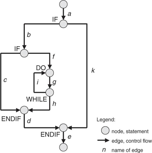
Test cases

Coverage of the nodes of the control flow

In this example, all statements (all nodes) can be reached by a single test case. In this test case, the edges of the graph must be traversed in this order:

a, b, f, g, h, d, e

One test case is enough

After the edges are traversed in this way, all statements have been executed once. Other combinations of edges of the graph can also be used to achieve complete coverage. But the cost of testing should always be minimized, which means reaching the goal with the smallest possible number of test cases.

The expected results and the expected behavior of the test object should be identified in advance from the specification (not the code!). After execution, the expected and actual results, and the behavior of the test object, must be compared to detect any difference or failure.

Definition of the Test Exit Criteria

The exit criteria for the tests can be very clearly defined:

→Statement coverage =
(number of executed statements / total number of statements) × 100%

C0-measure

Statement coverage is also known as C0-coverage (C-zero). It is a very weak criterion. However, sometimes 100% statement coverage is difficult to achieve, as when, for instance, exception conditions appear in the program that can be triggered only with great trouble or not at all during test execution.

The Value of the Technique

Unreachable code can be detected

If complete coverage of all statements is required and some statements cannot be executed by any test case, this may be an indication of unreachable source code (dead statements).

Empty ELSE parts are not considered

If a condition statement (IF) has statements only after it is fulfilled (i.e., after the THEN clause) and there is no ELSE clause, then the control flow graph has a THEN edge, starting at the condition, with (at least) one node, but additionally a second outgoing ELSE edge without any intermediate nodes. The control flow of both of these edges is reunited at the terminating (ENDIF) node. For statement coverage, an empty ELSE edge (between IF and ENDIF) is irrelevant. Possible missing statements in this program part are not detected by a test using this criterion!

Statement coverage is measured using test tools (section 7.1.4).

5.2.2 Decision/Branch Testing and Coverage

A more advanced criterion for white box testing is →branch coverage of the control flow graph; for example, the edges (connections) in the graph are the center of attention. This time, the execution of decisions is considered instead of the execution of the statement. The result of the decision determines which statement is executed next. This should be used in testing.

→branch or decision test

If the basis for a test is the control flow graph with its nodes and edges, then it is called a branch test or branch coverage. A branch is the connection between two nodes of the graph. In the program text, there are IF or CASE statements, loops, and so on, also called decisions. This test is thus called decision test or decision coverage. There may be differences in the degree of coverage. The following example illustrates this: An IF statement with an empty ELSE-part is checked. Decision testing gives 50% coverage if the condition is evaluated to true. With one more test case where the condition is false, 100% decision coverage will be achieved. For the branch test, which is built from the control flow graph, slightly different values result. The THEN part consists of two branches and one node, the ELSE part only of one branch without any node (no statement there). Thus, the whole IF statement with the empty ELSE part consists of three branches. Executing the condition with true results in covering two of the three branches, that is, 66% coverage. (Decision testing gives 50% in this case). Executing the second test case with the condition being false, 100% branch coverage and 100% decision coverage are achieved. Branch testing is discussed further a bit later.

Empty ELSE-parts are considered

Thus, contrary to statement coverage, for branch coverage it is not interesting if, for instance, an IF statement has no ELSE-part. It must be executed anyway. Branch coverage requires the test of every decision outcome: both THEN and ELSE in the IF statement; all possibilities for the CASE statement and the fall-through case; for loops, both execution of the loop body, bypassing the loop body and returning to the start of the loop.

Test Cases

Additional test cases necessary

In the example (figure 5-9), additional test cases are necessary if all branches of the control flow graph must be executed during the test. For 100% statement coverage, a test case executing the following order of edges was sufficient:

a, b, f, g, h, d, e

The edges c, i, and k have not been executed in this test case. The edges c and k are empty branches of a condition, while the edge i is the return to the beginning of the loop. Three test cases are necessary:

a, b, c, d, e
a, b, f, g, i, g, h, d, e
a, k, e

Connection (edge) coverage of the control flow graph

All three test cases result in complete coverage of the edges of the control flow graph. With that, all possible branches of the control flow in the source code of the test object have been tested.

Some edges have been executed more than once. This seems to be redundant, but it cannot always be avoided. In the example, the edges a and e are executed in every test case because there is no alternative to these edges.

For each test case, in addition to the preconditions and postconditions, the expected result and expected behavior must be determined and then compared to the actual result and behavior. Furthermore, it is reasonable to record which branches have been executed in which test case in order to find wrong execution flows. This helps to find faults, especially missing code in empty branches.

Definition of the Test Exit Criteria

As with statement coverage, the degree of branch coverage is defined as follows:

Branch coverage =
(number of executed branches / total number of branches) × 100%

C1-measure

Branch coverage is also called C1-coverage. The calculation counts only if a branch has been executed at all. The frequency of execution is not relevant. In our example, the edges a and e are each passed three times—once for each test case.

If we execute only the first three test cases in our example (not the fourth one), edge k will not be executed. This gives a branch coverage of 9 executed branches out of 10 total:

(9 / 10) × 100% = 90%.

For comparison, 100% statement coverage has already been achieved after the first test case.

Depending on the criticality of the test object, and depending on the expected failure risk, the test exit criterion can be defined differently. For instance, 85% branch coverage can be sufficient for a component of one project, whereas for a different project, another component must be tested with 100% coverage. The example shows that the test cost is higher for higher coverage requirements.

The Value of the Technique

More test cases necessary

Decision/branch coverage usually requires the execution of more test cases than statement coverage. How much more depends on the structure of the test object. In contrast to statement coverage, branch coverage makes it possible to detect missing statements in empty branches. Branch coverage of 100% guarantees 100% statement coverage, but not vice versa. Thus, branch coverage is a stronger criterion.

Each of the branches is regarded separately and no particular combinations of single branches are required.

Hint

§ A branch coverage of 100% should be aimed for.

§ The test can only be categorized as sufficient if, in addition to all statements, every possible branch of the control flow, and thus every possible result of a decision in the program text, is considered during test execution.

Inadequate for object-oriented systems

For object-oriented systems, statement coverage as well as branch coverage are inadequate because the control flow of the functions in the classes is usually short and not very complex. Thus, the required coverage criteria can be achieved with little effort. The complexity in object-oriented systems lies mostly in the relationship between the classes, so additional adequate coverage criteria are necessary in this case. As tools often support the process of determining coverage, coverage data can be used to detect not-called methods or program parts.

5.2.3 Test of Conditions²⁷

Considering the complexity of combined conditions

Branch coverage exclusively considers the logical value of the result of a condition (“true” or “false”). Using this value, it is decided which branch in the control flow graph to choose and, accordingly, which statement is executed next in the program. If a decision is based on several (partial) conditions connected by logical operators, then the complexity of the condition should be considered in the test. The following sections describe different requirements and degrees of test intensity under consideration of combined conditions.

Condition Testing and Coverage

The goal of condition testing is to cause each →atomic (partial) condition in the test to adopt both a true and a false value.

Definition of an atomic partial condition

An atomic partial condition is a condition that has no logical operators such as AND, OR, and NOT but at the most includes relation symbols such as > and =. A condition in the source code of the test object can consist of multiple atomic partial conditions.

Example for combined conditions

An example for a combined condition is x > 3 OR y < 5. The condition consists of two conditions (x > 3; y < 5) connected by the logical operator OR.

The goal of condition testing is that each partial condition (i.e., each individual part of a combined condition) is evaluated once, resulting in each of the logical values. The test data x = 6 and y = 8 result in the logical value true for the first condition (x > 3) and the logical value false for the second condition (y < 5). The logical value of the complete condition is true (true OR false = true). The second pair of test data with the values x = 2 and y = 3 results in false for the first condition and true for the second condition. The value of the complete condition results in trueagain (false OR true = true). Both parts of the combined condition have each resulted in both logical values. The result of the complete condition, however, is equal for both combinations.

A weak criterion

Condition coverage is therefore a weaker criterion than statement or branch coverage because it is not required that different logical values for the result of the complete condition are included in the test.

Multiple Condition Testing and Coverage

All combinations of the logical values

Multiple condition testing requires that all true-false combinations of the atomic partial conditions be exercised at least once. All variations should be built, if possible.

Continuation of the example

Four combinations of test cases are possible with the test data from the previous example for the two conditions (x > 3, y < 5):

x = 6 (T), y = 3 (T), x > 3 OR y < 5 (T)
x = 6 (T), y = 8 (F), x > 3 OR y < 5 (T)
x = 2 (F), y = 3 (T), x > 3 OR y < 5 (T)
x = 2 (F), y = 8 (F), x > 3 OR y < 5 (F)

Multiple condition testing subsumes statement and branch coverage

The evaluation of the complete condition results in both logical values. Thus, multiple condition testing meets the criteria of statement and branch coverage. It is a more comprehensive criterion that also takes into account the complexity of combined conditions. But this is a very expensive technique due to the growing number of atomic partial conditions that make the number of possible combinations grow exponentially (to 2ⁿ, with n being the number of atomic partial conditions).

Not all combinations are always possible

A problem results from the fact that test data cannot always generate all combinations.

Example for not feasible combinations of partial condition

An example should clarify this. For the combined condition of 3≤x AND x<5 not all combinations with the according values for the variable x can be produced because the parts of the combined condition depend on each other:

x = 4: 3 ≤ x (T), x < 5 (T), 3 ≤ x AND x < 5 (T)
x = 8: 3 ≤ x (T), x < 5 (F), 3 ≤ x AND x < 5 (F)
x = 1: 3 ≤ x (F), x < 5 (T), 3 ≤ x AND x < 5 (F)
x = ?: 3 ≤ x (F), x < 5 (F), combination not possible because the value x shall be smaller than 3 and greater than or equal to 5 at the same time.

Condition Determination Testing / Minimal Multiple Condition Testing

Restriction of the combinations

Condition determination testing eliminates the problems discussed previously. Not all combinations must be included; however, include every possible combination of logical values where the modification of the logical value of an atomic partial condition can change the logical value of the whole combined condition. Stated in another way, for a test case, every atomic partial condition must have a meaningful impact on the result. Test cases in which the result does not depend on a change of an atomic partial condition need not be designed.

Continuation of the example

For clarification, we revisit the example with the two atomic partial conditions (x > 3, y < 5) and the OR-connection (x > 3 OR y < 5). Four combinations are possible (2²):

1) x = 6 (T), y = 3 (T), x > 3 OR y < 5 (T)
2) x = 6 (T), y = 8 (F), x > 3 OR y < 5 (T)
3) x = 2 (F), y = 3 (T), x > 3 OR y < 5 (T)
4) x = 2 (F), y = 8 (F), x > 3 OR y < 5 (F)

Changing a partial condition without changing the result

For the first combination, the following applies: If the logical value is wrongly calculated for the first condition (i.e., an incorrect condition is implemented), then the fault can change the logical value of the first condition part from true (T) to false (F). But the result of the complete condition stays unchanged (T). The same applies for the second partial condition.

For the first combination, incorrect results of each partial condition are masked because they have no effect on the result of the complete condition and thus failures will not become visible at the outside. Consequently, the test with the first combination can be left out.

If the logical value of the first partial condition in the second test case is calculated wrongly as false, then the result value of the combined condition changes from true (T) to false (F). A failure then becomes visible because the value of the combined condition has also changed. The same applies for the second partial condition in the third test case. In the fourth test case, an incorrect implementation is detected as well because the logical value of the complete condition changes.

Small number of test cases

For every logical combination of the combined decision, it must be decided which test cases are sensitive to faults and for which combinations faults can be masked. Combinations where faults are masked need not be considered in the test. Here, the number of test cases is significantly smaller than in multiple condition testing.

Test Cases

For designing the test cases, it must be considered which input data leads to which result of the decisions or partial conditions and which parts of the program will be executed after the decision. The expected output and expected behavior of the test object should also be defined in advance in order to detect whether the program behaves correctly.

Hint

§ Because of the weak significance, condition testing should not be used.

§ For complex conditions, condition determination testing should be applied because the complexity of the conditional expression is taken into account for test case design. The method also subsumes statement and branch coverage, which means they need not be checked in addition.

However, it may be very expensive to choose the input values in such a way that a certain part of the condition gets the logical value required by the test case.

Definition of the Test Exit Criteria

Analogous to the previous techniques, the proportion between the executed and all the required logical values of the (partial) condition (parts) can be calculated. For the techniques, which concentrate on the complexity of the decisions in the source code, it is reasonable to try to achieve a complete verification (100% coverage). If complexity of the decisions is not important in testing, branch coverage can be seen as sufficient.

The Value of the Technique

Complex conditions are often defect prone

If complex decisions are present in the source code, they must be tested intensively to detect possible failures. Combinations of logical expressions are especially defect prone. Thus, a comprehensive test is very important. However, condition determination testing is an expensive technique for test case design.

Hint

§ It can be reasonable to split combined complex conditions into a tree structure of nested simple conditions and then execute a branch coverage test for these sequences of conditions.

§ The intensive test of complex conditions can possibly be omitted if they have been subjected to a review (section 4.1.2) in which the correctness is verified.

Excursion

A disadvantage of condition testing is that it checks Boolean expressions only inside a statement (for example, IF statement). In the following example of a program fragment, the following fact remains undetected: the IF condition actually consists of multiple parts and condition determination testing needs to be applied.

...
Flag = (A || (B && C));
If (Flag)
...;
else ...;
...

This particular disadvantage can be circumvented if all Boolean expressions that occur are used as a basis for the creation of test cases.

The compiler terminates evaluation of expressions

Another problem occurs in connection with measuring the coverage of (partial) conditions. Some compilers shortcut the evaluation of the Boolean expression as soon as the total result of the decision is known. For instance, if the value FALSE has been detected for one of two condition parts of an AND-combination, then the complete condition is FALSE regardless of the result of the second condition part. Some compilers even change the order of the evaluation, depending on the Boolean operators, to get the final result as quickly as possible and to be able to disregard any other partial conditions. Test cases that are supposed to achieve 100% coverage can be executed, but because of the shortened evaluation, this coverage cannot be verified.

Path Testing and Coverage²⁸

Excursion:

All possible paths through a test object

Until now, test case determination focused on the statements or branches of the control flow as well as the complexity of decisions. If the test object includes loops or repetitions, the previous considerations are not sufficient for an adequate test. Path coverage requires the execution of all different paths through the test object.

Example for a path test

To clarify the use of the term path, consider the control flow graph in figure 5-9.

The program fragment represented by the graph contains a loop. This DO-WHILE loop is executed at least once. In the WHILE condition at the end of the loop, it is decided whether the loop must be repeated, that is, if a jump back to the start of the loop is necessary. When using branch coverage for test design, the loop has been considered in two test cases:

§ Loop without repetition:

a, b, f, g, h, d, e

§ Loop with single return (i) and a single repetition:

a, b, f, g, i, g, h, d, e

Usually a loop is repeated more than once. Further possible sequences of branches through the graph of the program are as follows:

a, b, f, g, i, g, i, g, h, d, e
a, b, f, g, i, g, i, g, i, g, h, d, e
a, b, f, g, i, g, i, g, i, g, i, g, h, d, e
etc.

This shows that there are an indefinite number of paths in the control flow graph. Even with restrictions on the number of loop repetitions, the number of paths increases indefinitely (see also section 2.1.4).

Combination of program parts

A path describes the possible order of single program parts in a program fragment.

Contrary to this, branches are viewed independently, each for itself. The paths consider dependencies between the branches, as for example with loops, at which one branch leads back to the beginning of another branch.

Example: Statement and branch coverage in VSR

In section 5.1.1 for the function calculate_price() of the VSR subsystem DreamCar, test cases have been derived from valid and invalid equivalence classes of the parameters. In the following code, test cases are evaluated by their ability to cover the source code, that is, execute respective parts of the method. Branch coverage of 100% should be achieved to ensure that during test execution all branches have been executed at least once.

For better understanding, the source code of the function from section 3.2.3 is repeated here:

double calculate_price (
double baseprice, double specialprice,
double extraprice, int extras, double discount)
{
double addon_discount;
double result;

if (extras >= 3) addon_discount = 10;
else if (extras >= 5) addon_discount = 15;
else addon_discount = 0;
if (discount > addon_discount)
addon_discount = discount;
result = baseprice /100.0*(100-discount)
+ specialprice
+ extraprice/100.0*(100-addon_discount);
return (result);
}

The control flow graph of the function calculate_price() is shown in figure 5-10.

Figure 5–10
Control flow graph of the function calculate_price()

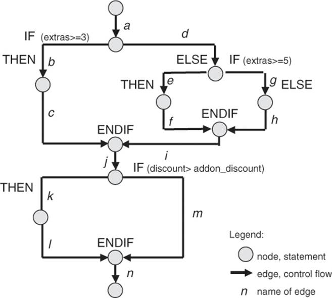
In section 3.2.3, the following two test cases have been chosen:

// testcase 01
price = calculate_price(10000.00,2000.00,1000.00,3,0);
test_ok = test_ok && (abs(price–12900.00) < 0.01);

// testcase 02
price = calculate_price(25500.00,3450.00,6000.00,6,0);
test_ok = test_ok && (abs(price-34050.00) < 0.01);

The test cases cause the execution of the following edges of the graph:

Test case 01: a, b, c, j, m, n
Test case 02: a, b, c, j, m, n

43% branch coverage achieved

The edges d, e, f, g, h, i, k, l have not been executed. The two test cases covered only 43% of the branches (6 out of 14). Test case 02 gives no improvement of the coverage and is not necessary for branch coverage. However, considering the specification, test case 02 should have led to execution of more statements because a different discount should have been calculated (with five or more pieces of extra equipment).

To increase test coverage, the following further test cases are specified:

// testcase 03
price = calculate_price(10000.00,2000.00,1000.00,0,10);
test_ok = test_ok && (abs(price–12000.00) < 0.01);

// testcase 04
price = calculate_price(25500.00,3450.00,6000.00,6,15);
test_ok = test_ok && (abs(price–30225.00) < 0.01);

These test cases cause the execution of the following edges of the graph:

Test case 03: a, d, g, h, i, j, k, l, n
Test case 04: a, b, c, j, k, l, n

86% path coverage achieved

These test cases lead to execution of further edges (d, g, h, i, k, and l) and thus increase branch coverage to 86%. Edges e and f have not yet been executed.

Evaluation of the conditions

Before trying to reach the missing edges by further test cases, the conditions of the IF statements are analyzed more closely, that is, the source code is analyzed in order to define further test cases. To get to the edges e and f, the result of the first condition (extras ≥ 3) must be false in order to execute the ELSE-part. In this ELSE-part, the condition (extras ≥ 5) must be true. Therefore, a value has to be found that meets the following condition:

¬(extras ≥ 3) AND (extras ≥ 5)

No such value exists and the missing edges can never be reached. The source code contains a defect.

Example: Relationship between the measures

This example should clarify the relationship between statement, branch, and path coverage as well. The test object consists of altogether three IF statements; two are nested and the third is placed separately from the others (figure 5-10).

All statements (nodes) are executed by the following sequence of edges in the graph:

a, b, c, j, k, l, n
a, d, e, f, i, j, k, l, n
a, d, g, h, i, j, k, l, n

These sequences are sufficient to achieve 100% statement coverage. But not all branches (edges) have been covered yet. The edge m is still missing. An execution sequence might look like this:

a, b, c, j, m, n

This new sequence can replace the first execution sequence shown previously. With the resulting three test cases, which result in these three execution sequences, 100% branch coverage is achieved.

Further paths through the graph

But, even for this simple program fragment, there are still possibilities to traverse the graph differently and thus take care of all paths through the graph. Until now, the following paths have not been executed yet:

a, d, e, f, i, j, m, n
a, d, g, h, i, j, m, n

Altogether, six different paths through the source code result (the three possible paths through the graph before edge j multiplied by two for the two possible paths after edge j). There is the precondition that the conditions are independent from each other and the edges can be combined freely.

If there are loops in the source code, then every possible number of loop repetitions is counted as a possible path through the program fragment. It is obvious that 100% path coverage in testing is not feasible for a nontrivial program.

5.2.4 Further White Box Techniques

In addition to the most common techniques described here, there are a number of other white box test techniques that can be used for evaluating test objects. You can find out more about them in [Myers 79], [Beizer 90], and [Pol 98]. The following section describes one technique in a little more detail.

Excursion

Data-flow-based techniques

A number of techniques use the flow of data through the test object as the basis for identifying test cases. Primarily, the data usages in the test object are verified. The use of each variable is analyzed, whereby the definitions of and read/write access to variables are distinguished from each other. These techniques may find faults where a value of a variable in the test object causes failures when it is used in other places. Furthermore, the technique verifies whether the value of a variable is used to create other variables or if it is used to calculate the logical value of a condition. This information allows defining various data flow criteria, which can then be covered by test cases. A detailed description of data-flow-based techniques can be found in [Clarke et al. 85].

5.2.5 General Discussion of the White Box Technique

Determine the test intensity

The basis for all of the white box techniques described is the source code.

Adequate test case design techniques can be chosen and applied depending on the complexity of the program structure. The intensity of the test depends on the source code and the selected technique.

Useful for lower test levels

The white box techniques we’ve described are appropriate for the lower test levels. For example, it is not very reasonable to require coverage of single statements or branches in a system test because system testing is not the right method to check single statements or conditions in the code.

Coverage is desirable even at higher test levels

The concept of coverage can be applied to other test levels above the code level. For example, during an integration test, we can assess what percentage of modules, components, or classes are executed during the test. This results in module, component, or class coverage. The required percentage value can be determined in advance and checked during test execution.

“Missing source code” is not considered

Missing implementation of requirements is impossible to find for white box techniques. White box techniques can verify only code that exists, that is, requirements that are implemented in the program, not code that should be there but isn’t. Thus, other test design techniques are required to find omissions.

5.2.6 Instrumentation and Tool Support

Determination of the executed program parts

Code-based white box techniques require that different program parts are executed and that conditions get different logical values. To be able to evaluate the test, it must be determined which program parts have already been executed and which haven’t. To do this, the test object must be instrumented at strategically relevant spots before test execution. →Instrumentation often works this way: The tool inserts counters in the program and initializes them with zero. During program execution, the counters are incremented when they are passed. At the end of the test execution, the counters contain the number of passes through the corresponding program parts. If a counter remained zero during the test, then the corresponding program part has not been executed.

Use tools

The instrumentation, the evaluation of the test runs, and the calculation of the achieved coverage should not be done manually because this would require too many resources and a manual instrumentation is error prone. Numerous tools perform these tasks (see section 7.1.4). These tools are important for white box testing because they increase productivity and indirectly improve the quality of the test object.

5.3 Intuitive and Experience-Based Test Case Determination

Besides the systematic approaches, intuitive determination of test cases should be performed. The systematically identified test cases may be supplemented by test cases designed using the testers’ intuition. The techniques are also called experience based because they depend on the experience of the testers. Intuitive testing can detect faults overlooked by systematic testing. It is therefore always advisable to perform additional intuitive testing.

Intuitive skill and experience of the testers

The basis of this method is the skill, experience, and knowledge of the tester to select test cases that uncover expected problems and their symptoms (failures). A systematic approach is not used. The test cases are based on where faults have occurred in the past or the tester’s ideas of where faults might occur in the future. This type of test case design is also called →error guessingand is used very often in practice.

Knowledge in developing similar applications and using similar technologies should also be used when designing test cases, in addition to experience in testing. If, for example, failures were found in previous projects in which a certain programming language was used, it is reasonable to use those failures when you are designing the tests in the actual project if you are using the programming language that caused the failures. One technique for intuitive testing, exploratory testing, will be discussed in more detail.

Exploratory testing

If the documents, which form the basis for test design, are of low quality, are obsolete, or do not exist at all, so-called exploratory testing may help. In the extreme case, only the program exists. The technique is also applicable when time is severely restricted because it uses much less time than other techniques. The approach is mainly based on the intuition and experience of the tester.

The approach of exploratory testing

The test activities in exploratory testing are executed nearly in parallel. The structured test process is not applied. An explicit previous planning of the test activities is not done. The possible elements of the test object (its specific tasks and functions) are “explored.” It is then decided which parts will be tested. Only a few test cases are executed and their results are analyzed. By executing the test cases, the “unknown” behavior of the test object will be determined further. Anything considered “interesting,” as well as other information, is then used to determine the next test cases. In this step-by-step manner, knowledge about the test object under test is collected. It becomes clearer what the test object does and how it works, which quality problems there could be, and which expectations to the program should be fulfilled. One result of exploratory testing may be that it becomes clear which test techniques can be applied if there is time left in the project.

Test charter

It makes sense to restrict exploratory testing to certain elements of the program (certain tasks or functions). The elements are further decomposed. The term test charter is used for such smaller parts. It should not take more than one or two hours to test a test charter. When executing test charters, the following questions are of interest:

§ Why? What is the goal of the test run?

§ What? What is to be tested?

§ How? Which testing method should be used?

§ What? What kind of problems should be found?

Main features of exploratory testing

The generic ideas of exploratory testing are as follows:

§ Results of one test case influence the design and execution of further test cases.

§ During testing, a “mental” model of the program under test is created. The model contains how the program “works” and how it behaves or how it should behave.

§ The test is run against this model. The focus is to find further aspects and behaviors of the program that are still not part of the “mental” model or are differing from aspects found before.

Neither black box nor white box

All the approaches for intuitive test case determination cannot be associated explicitly with white box or black box techniques because neither the requirements nor the source code are exclusively the basis for the considerations and tests. They should be applied more in the higher test levels. In the lower ones, usually sufficient information such as source code or detailed specification is accessible for applying systematic techniques.

Not to be used as first or only technique

Intuitive test case determination should not be applied as the primary testing technique. Instead, this technique should be used complete the test cases and to support the systematic test design techniques.

Test Cases

Knowledge for determination of additional test cases can be drawn from many sources.

Example: Tester knowledge for the CarConfigurator

In the development project for the CarConfigurator, the testers are very familiar with the previous system. Many of them have tested this system before. They know the weaknesses the system had and they know the problems the car dealers had with the operation of the old software (from hotline data and from discussions with car salespeople). Employees from the marketing department know for the business-related test which vehicles in which configurations are sold often and which theoretically possible combinations of extra equipment might not even be shippable. They use this experience to intuitively prioritize the systematically identified test cases and to complete them by additional test cases. The test manager knows which of the developer teams act under the most severe time pressure and even work on weekends. Hence, she will test the components from these teams more intensively.

Using all knowledge

Testers should use all their knowledge to find additional test cases. Naturally, the pre- and postconditions, the expected outcomes, and the expected behavior of the test object must be defined in advance for intuitive testing as well.

Hint

§ Because extensive experience is often only available in the minds of the experienced testers, maintaining a list with possible errors, faults, and suspicious situations might be very helpful. Frequently occurring errors, faults, and failures are noted in the list and are thus available to all the testers. With the help of the possible trouble areas and critical situations that have been identified, additional test cases can be designed.

§ The list may even be beneficial to developers because it indicates in advance what potential problems and difficulties might occur. These can be considered during implementation and thus serve for error prevention.

Definition of the Test Exit Criteria

A test exit criterion is not definable

Unlike with the systematic techniques, a criterion for termination cannot be specified. If the previously mentioned list exists, then a certain completeness can be verified against the list.

The Value of the Technique

Mostly successful in finding more defects

Intuitive test case determination and exploratory testing can often be used with good success. They are a sensible addition to systematic techniques. The success and effectiveness of this approach depend very much on testers’ skill and intuition and their previous experience with similar applications and the technologies used. Such approaches can also contribute to finding holes and errors in the risk analysis. If intuitive testing is applied in addition to systematic testing, inconsistencies in the test specification not previously detected can be found. Intensity and completeness of intuitive and exploratory test design cannot be measured.

5.4 Summary

Which technique and when to use it

This chapter has introduced a number of techniques for testing of software.²⁹ The question is, When should each technique be applied? The following list includes answers to this question and presents a reasonable approach. The general goal is to identify sufficiently different test cases in order to be able to find existing faults with a certain probability and with as little effort as possible. The techniques for test design should therefore be chosen appropriately.

However, before designing a test, you should check some factors that have considerable influence on the selection or even prescribe the application of certain test methods. The selection of techniques can depend on the following different circumstances and conditions:

§ The kind of test object

The complexity of the program text can vary considerably. Depending on this, adequate test techniques should be chosen. If, for example, decisions in the program are combined from several atomic conditions, branch coverage is not sufficient. A suitable technique to check the conditions should be chosen depending on the criticality and the risk in case of failure.

§ Formal documentation and the availability of tools

If specification or model information is available in a formal document, it can be fed directly into test design tools, which then derive test cases. This very much decreases the effort required to design the tests.

§ Conformance to standards

Industry and regulatory standards may require use of certain test techniques and coverage criteria. Compliance to such standards is often mandatory for safety-critical software or when high reliability is required.

§ Tester experience

Tester experience may lead to the choice of special techniques. A tester will, for example, reuse techniques that have led to finding serious faults earlier.

§ Customer wishes

The customer may require the use of specific test techniques and even the test coverage to be achieved. This has the advantage that at least these techniques will be applied during development. This may lead to fewer failures in acceptance testing.

§ Risk assessment

The expected risk dictates more or less the test activities, that is, the choice of techniques and the intensity of the execution. Risk-prone areas should be tested more thoroughly.

§ Additional factors

Finally, there are factors like the availability of the specification and other documentation, the knowledge and skill of the test personnel, time and budget, the test level, and previous experience with what kind of defects occur most often and with which test techniques these have been found. They can all have a large influence on selecting the testing techniques.

Test design techniques cannot be specified in a standard way. Their selection should always be based on a thoughtful decision. The following list should help in selecting the most applicable test technique.

Testing functionality

§ The system functioning correctly is certainly of great relevance. The functionality of the test object must be sufficiently verified. The development of all test cases, regardless of which technique or procedure was used, includes determining the expected results and reactions of the test object. This ensures a verification of the functionality for every evaluation of the test cases. Comparing the actual with the expected outputs and reactions contains a verification of the functionality.

Equivalence class partition combined with boundary value analysis

§ When you are designing test cases, equivalence class partitioning in combination with boundary value analysis should be applied for every test object. When you are executing these test cases, you should use the appropriate tools for measuring code coverage to find the test coverage already achieved (see section 7.1.4).

Consider execution history

§ If different states have an influence on the operating sequence in the test object, state transition testing must be applied. Only state transition testing verifies the cooperation of the states, transitions, and the corresponding behavior of the functions adequately.

§ If dependencies between the input data are given and must be taken care of in the test, these dependencies can be modeled using cause-effect graphs or decision tables. The corresponding test cases can be taken from the decision table.

§ If there are many parameters or settings with unknown dependencies, use pairwise testing for them.

§ For system testing, use cases (displayed in use case diagrams) can be applied as a basis for designing test cases.

§ In component and integration testing, coverage measurements should be included with all black box techniques. The parts of the test object still not executed should then be specifically tested with a white box test design technique. Depending on the criticality and nature of the test object, appropriate extensive white box technique must be selected.

Minimum criterion: branch coverage

§ The minimum criterion should be 100% branch coverage. If complex decisions exist in the test object, then condition determination testing is the appropriate technique to find faulty decisions.

§ In measuring coverage, loops should be repeated more than once. For critical parts of the system, the loops must be verified using the appropriate methods (boundary interior-path test and structured path test [Howden 75]).

§ Complete path coverage of a test object is usually not achievable. It should be considered a mere theoretical measure and is of little practical importance because of the great cost and because it is impossible to achieve for programs with loops. It is very seldom used in practice.

§ It is sensible to apply white box techniques at lower test levels while black box techniques can be applied in all test levels, especially the higher ones.

§ Intuitive determination of test cases should not be ignored. It is a good supplement to systematic test design methods.

Hint

§ Testing always comprises the combination of different techniques because no testing technique exists that covers all aspects to be considered in testing equally well.

§ The criticality and the expected risk in case of failure guide the selection of the testing techniques and the intensity of the execution.

§ The basis for the selection of the white box technique is the structure of the test object. If, for example, no complex decisions exist in the test object, the use of condition determination testing makes no sense.