Plan, Activity, and Intent Recognition: Theory and Practice, FIRST EDITION (2014)

Part I. Plan and Goal Recognition

Chapter 1. Hierarchical Goal Recognition

Nate Blaylock^a and James Allen^b, ^aNuance Communications, Montreal, QC, Canada, ^bFlorida Institute for Human and Machine Cognition, Pensacola, FL, USA

Abstract

This chapter discusses hierarchical goal recognition: simultaneous online recognition of goals and subgoals at various levels within an HTN-like plan tree. We use statistical, graphical models to recognize hierarchical goal schemas in time quadratic with the number of the possible goals. Within our formalism, we treat goals as parameterized actions, necessitating the recognition of parameter values as well. The goal schema recognizer is combined with a tractable version of the Dempster-Shafer theory to predict parameter values for each goal schema. This results in a tractable goal recognizer that can be trained on any plan corpus (a set of hierarchical plan trees). Additionally, we comment on the state of data availability for plan recognition in general and briefly describe a system for generating synthetic data using a mixture of AI planning and Monte Carlo sampling. This was used to generate the Monroe Corpus, one of the first large plan corpora used for training and evaluating plan recognizers. This chapter also discusses the need for general metrics for evaluating plan recognition and proposes a set of common metrics.

Keywords

Plan recognition

Goal recognition

Activity recognition

Plan corpus

Plan recognition metrics

Plan recognition evaluation

Acknowledgments

This material is based on work supported by a grant from DARPA under grant number F30602-98-2-0133, two grants from the National Science Foundation under grant numbers IIS-0328811 and E1A-0080124, ONR contract N00014-06-C-0032, and the EU-funded TALK project (IST-507802). Any opinions, findings, and conclusions or recommendations expressed in this material are those of the authors and do not necessarily reflect the views any of these organizations.

1.1 Introduction

Much work has been done over the years in plan recognition which is the task of inferring an agent’s goal and plan based on observed actions. Goal recognition is a special case of plan recognition in which only the goal is recognized. Goal and plan recognition have been used in a variety of applications including intelligent user interfaces [6,18,20], traffic monitoring [26], and dialog systems [13].

For most applications, several properties are required in order for goal recognition to be useful, as follows:

Speed: Most applications use goal recognition “online,” meaning they need recognition results before the observed agent has completed its activity. Ideally, goal recognition should take a fraction of the time it takes for the observed agent to execute its next action.

Precision and recall: We want the predictions to be correct (precision), and we want to make correct predictions at every opportunity (recall).

Early prediction: Applications need accurate plan prediction as early as possible in the observed agent’s task execution (i.e., after the fewest number of observed actions). Even if a recognizer is fast computationally, if it is unable to predict the plan until after it has seen the last action in the agent’s task, it will not be suitable for online applications; those need recognition results during task execution. For example, a helpful assistant application needs to recognize a user’s goal early to be able to help. Similarly, an adversarial agent needs to recognize an adversary’s goal early in order to help thwart its completion.

Partial prediction: If full recognition is not immediately available, applications often can make use of partial information. For example, if the parameter values are not known, just knowing the goal schema may be enough for an application to notice that a hacker is trying to break into a network. Also, even though the agent’s top-level goal (e.g., steal trade secrets) may not be known, knowing a subgoal (e.g., gain root access to server 1) may be enough for the application to act. (Our approach enables both types of partial prediction.)

In our work, we model goals, subgoals, and actions as parameterized action schemas from the SHOP2 HTN planner [23]. With this formalism, we can distinguish between recognition of a goal schema and its corresponding parameter values. The term instantiated goal recognition means the recognition of a goal schema together with its parameter values. Additionally, we consider the task of hierarchical goal recognition, which is the recognition of the chain of the agent’s currently active top-level goal and subgoals within a hierarchical plan. As an illustration, consider Figure 1.1; it shows a hierarchical plan tree and a corresponding set of goal chains for left-to-right execution.

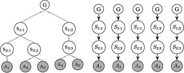
FIGURE 1.1 A hierarchical plan and corresponding goal chains.

Here, the root of the tree () is the agent’s top-level goal. Leaves of the tree () represent the atomic actions executed by the agent. Nodes in the middle of the tree represent the agent’s various subgoals within the plan. For each executed atomic action, we can define a goal chain which is the subgoals that were active at the time it was executed. This is the path that leads from the atomic action to the top-level goal . We cast hierarchical goal recognition as the recognition of the goal chain corresponding to the agent’s last observed action.

Recognizing such goal chains can provide valuable information not available from a system that recognizes top-level goals only. First, though not full plan recognition, which recognizes the full plan tree, hierarchical goal recognition provides information about which goal an agent is pursuing as well as a partial description of how (through the subgoals).

Additionally, the prediction of subgoals can be seen as a type of partial prediction. As mentioned before, when a full prediction is not available, a recognizing agent can often make use of partial predictions. A hierarchical recognizer may be able to predict an agent’s subgoals even when the top-level goal is still not clear. This can allow a recognizer to make predictions much earlier in an execution stream (i.e., after less observed actions).

The remainder of this chapter first discusses previous work in goal recognition. We then detail the need for annotated data for plan recognition and present a method for generating synthetic labeled data for training and testing plan recognizers. This is followed by a discussion of how best to measure plan recognition performance among a number of attributes. We then describe our own hierarchical goal recognizer and its performance. Finally, we conclude and discuss future directions.

1.2 Previous Work

We focus here exclusively on previous work on hierarchical goal recognition. For a good overview of plan recognition in general, see Carberry [14].

Pynadath and Wellman [27] use probabilistic state-dependent grammars (PSDGs) to do plan recognition. PSDGs are probabilistic context-free grammars (PCFGs) in which the probability of a production is a function of the current state. This allows, for example, the probability of a recipe (production) to become zero if one of its preconditions does not hold. Subgoals are modeled as nonterminals in the grammar, and recipes are productions that map those nonterminals into an ordered list of nonterminals or terminals. During recognition, the recognizer keeps track of the current productions and the state variables as a Dynamic Bayes Network (DBN) with a special update algorithm. The most likely string of current productions is predicted as the current hierarchical goal structure.

If the total state is observable, Pynadath and Wellman claim the complexity of the update algorithm to be linear in the size of the plan hierarchy (number of productions).¹ However, if the state is only partially observable, the runtime complexity is quadratic in the number of states consistent with observation, which grows exponentially with the number of unobservable state nodes.

Additionally, the recognizer only recognizes atomic goals and does not take parameters into account. Finally, although the PSDGs allow fine probability differences for productions depending on the state, it is unclear how such probability functions could be learned from a corpus because the state space can be quite large.

Bui [10] performs hierarchical recognition of Markov Decision Processes. He models these using an Abstract Hidden Markov Model (AHMM)—multilevel Hidden Markov Models where a policy at a higher level transfers control to a lower level until the lower level “terminates.” The addition of memory to these models [11] makes them very similar to the PSDGs used by Pynadath in that each policy invokes a “recipe” of lower-level policy and does not continue until the lower level terminates.

Recognition is done using a DBN, but because this is intractable, Bui uses a method called Rao-Blackwellization (RB) to split network variables into two groups. The first group, which includes the state variables as well as a variable that describes the highest terminating state in the hierarchy, is estimated using sampling methods. Then, using those estimates, exact inference is performed on the second part—the policy variables. The separation is such that exact inference on the second group becomes tractable, given that the first group is known.

The recognizer was used in a system that tracked human behavior in an office building at three abstract levels, representing individual offices at the bottom level, then office groups, and then finally the entire building. Policies at each level were defined specific to each region—for example, the policy (behavior) of using the printer in the printer room. In this model, only certain policies are valid in a given state (location), which helps reduce the ambiguity. Typically, the domain is modeled such that lower-level policies become impossible as the agent moves to another room, which makes it fairly clear when they then terminate.

Although the algorithm was successful for this tracking task, it is unclear how effective estimation of policy termination would be in general (e.g., when most policies are valid in most states). Also, similar to Pynadath, this method only recognizes atomic goals and does not support parameters.

1.3 Data for Plan Recognition

Historically, work on plan recognition (under its many names and guises) has been quite fragmented, and, although statistical techniques have been used, the data-driven revolution, which has occurred in many AI fields, has lagged for plan recognition; in part this is because of a lack of common data sets and metrics that allow systems to be compared. This section discusses plan corpora: data appropriate for plan recognition. We first describe types and possible sources of plan corpora. We then detail a novel method for creating synthetic data and describe the Monroe Plan Corpus, which was created using this method and serves as the principal data set for the goal recognizer in this chapter.

1.3.1 Human Sources of Plan Corpora

In this section we mention several plausible ways of gathering plan corpora by observing humans. These can be divided into the kind of data that they make available: unlabeled, goal labeled, and plan labeled data. We describe each in turn and then discuss the general difficulties of gathering human data.

1.3.1.1 Unlabeled data

Several techniques are used in related fields for gathering unlabeled data, which could be useful for plan recognition.

A number of projects in ubiquitous computing [2,25,29] have gathered raw data of a user’s state over time (location and speed from GPS data), which they use to predict user activity. These represent very low-level data, however, that is not immediately compatible with the intentional action streams that most plan recognizers take as input.

There have been several efforts to watch user behavior on a computer (e.g., mouse clicks, Unix commands) in order to recognize activity ([16,21], inter alia). It is unclear how useful such unlabeled data would be by itself for plan recognition (although Bauer [5], has done work on using such data to automatically construct recipe libraries).

1.3.1.2 Goal-labeled data

Much more useful to plan recognition are goal-labeled plan corpora, although such corpora are even more difficult to come by.

Albrecht et al. [1] extract a plan corpus from the logs of a Multi-User Dungeon (MUD) game. A log includes a sequence of both player location (within the game) and each command executed. In addition, the MUD records each successful quest completion, which can be used to automatically tag plan sessions with a top-level goal (as well as partial state with the user’s location). Albrecht et al. report that the corpus data is quite noisy: first because of player errors and typos and then because players in MUDs often interleave social interaction and other activities. We should also note that the goals in the corpus are atomic, as opposed to being parameterized goal schemas.

More tightly controlled, goal-labeled corpora have been gathered through data collection efforts in Unix [19] and Linux²[7] domains. In these experiments, test subjects are given a specific goal (e.g., “find a file that ends in.tex”) and their shell commands are recorded as they try to accomplish it. The subjects then report when they have successfully accomplished the goal because there is no way to easily compute this automatically.

In these controlled experiments, top-level goal labeling is much more reliable because it is assigned a priori. Of course, this work can still be noisy, as when the subject misunderstands the goal or incorrectly believes he has accomplished it. Also, this kind of data collection is expensive as compared to those mentioned earlier. The preceding data collections monitor the normal activity of subjects, whereas these types of collections require subjects to work on tasks specifically for the collection.

1.3.1.3 Plan-labeled data

Of course, the most useful type of plan corpus would include not only the top-level goal but also the plan and state of the world.

Bauer [4] records user action sequences (and corresponding system state) in an email program and uses a plan recognizer post hoc to label them with the appropriate goal and plan. This post hoc recognition can potentially be much more accurate than online prediction because it is able to look at the whole execution sequence. A potential problem we see with this approach is that, if the original plan recognizer consistently makes mistakes in predicting plans, these mistakes will be propagated in the corpus. This includes cases where the plan library does not cover extra or erroneous user actions.

1.3.1.4 General challenges for human plan corpora

In addition to the individual disadvantages mentioned, we see several shortcomings to this kind of human data collection for plan recognition.

First, this kind of data collection is most feasible in domains (e.g., operating systems) where higher-level user actions can be directly observed and automatically recorded (as opposed to low-level sensor readings). This, unfortunately, excludes most nonsoftware interaction domains. In fact, the only way we can envision to gather data for other domains would be to have it annotated by hand, which could be expensive and time consuming. Not to mention error-prone.

Finally, a major shortcoming of this work is that it is at most labeled with a top-level goal.³ In most domains where plan recognition is used (e.g., natural language understanding), the system can benefit not only from the prediction of a top-level goal but also from partial results where a subgoal is predicted. This is especially true of domains with plans composed of large action sequences, where the top-level goal may not become apparent until very far into the plan’s execution. We imagine that manual annotation of plan labeling would be quite tedious and error-prone.

1.3.2 Artificial Corpus Generation

In contrast to human data collection, we propose the use of an AI planner and Monte Carlo simulation to stochastically generate synthetic plan corpora [8]. This method can be used for any domain and provides a corpus accurately labeled with goal and hierarchical plan structure. It also provides an inexpensive way to produce the kind of large corpora needed for machine learning. The method is as follows:

1. Modify an AI planner to search for valid plans nondeterministically.

2. Model the desired domain for the planner.

3. The algorithm does the following to generate each item in the corpus:

(a) Stochastically generates a goal.

(b) Stochastically generates a start state.

(c) Uses the planner to find a valid plan for the generated goal and start state.

Next, we first describe the modifications to an AI planner. Then we discuss issues of domain modeling and the stochastic generation of the goal and start state. Finally, we discuss the general characteristics of the corpora generated by this process and mention the Monroe Plan Corpus.

1.3.2.1 Planner modification

For plan recognition, we want to create corpora that allow for all possible plans in the domain. Typical AI planners do not support this, as they usually deterministically return the same plan for a given goal and start state. Many planners also try to optimize some plan property (e.g., length or cost) and therefore would never output longer, less optimal plans. We want to include all possible plans in our corpus to give us broad coverage.

We therefore modified the SHOP2 planner [23] to randomly generate one of the set of all possible plans for a given goal and start state.⁴ We did this by identifying key decision points in the planner and randomizing the order that they were searched.

SHOP2 [23] is a sound and complete hierarchical transition network (HTN) planner. SHOP2 is novel in that it generates plan steps in the order they will be executed, which allows it to handle complex reasoning capabilities, such as axiomatic inference, and calls to external programs. It also allows partially ordered subtasks. The planning model in SHOP2 consists of methods (decomposable goals), operators (atomic actions), and axioms (facts about the state).

In searching the state space, there are three types of applicable decision points, which represent branches in the search space⁵:

• Which (sub) goal to work on next

• Which method to use for a goal

• Which value to bind to a parameter

To provide for completeness, SHOP2 keeps lists of all possibilities for a decision point so that it may backtrack if necessary. We modified the planner so that these lists are randomized after they are populated but before they are used. This one-time randomization guarantees that we search in a random order but also allows us to preserve the soundness and completeness of the algorithm. We believe the randomized version is equivalent to computing all valid plans and randomly choosing one.

1.3.2.2 Domain modeling

Each new domain must be modeled for the planner, just as it would if the intent were to use the planner for its usual purpose. As opposed to modeling for plan generation, however, care should be taken to model the domain such that it can encompass all anticipated user plans.

Usually the planning model must be written by hand, although work has been done on (semi-) automating the process (e.g., by Bauer [5]). Note that, in addition to the model of the plan library, which is also used in many plan recognizers, it is necessary to model state information for the planner.

1.3.2.3 Goal generation

We separate goal generation into two steps: generating the goal schema and generating parameter values for the schema.

Goal Schema Generation. In addition to the domain model for the planner, the domain modeler needs to provide a list of possible top-level goals in the domain, together with their a priori probability. A priori probabilities of goals are usually not known, but they could be estimated by the domain modeler’s intuitions (or perhaps by a small human corpus). The algorithm uses this list to stochastically pick one of the goal schemas.

Goal Parameter Value Generation. In domains where goals are modeled with parameters, the values of the parameters also must be generated. Goal parameter values can be generated by using one of two techniques. For goal schemas where the parameter values are more or less independent, the domain modeler can give a list of possible parameter values for each slot, along with their a priori probabilities. For schemas where parameter values are not independent, each possible set of parameter values is given, along with their probabilities.

Once the goal schema has been chosen, the algorithm uses this list to stochastically generate values for each parameter in it. At this point, a fully instantiated goal has been generated.

1.3.2.4 Start state generation

In addition to a top-level goal, planners need to know the state of the world—the start state. To model agent behavior correctly, we need to stochastically generate start states, as this can have a big effect on the plan an agent chooses.

Generating the start state is not as straightforward as goal generation for several reasons. First, the domain must be structured such that we can generate start states with an accompanying a priori probability. Second, in order to make the planning fast, we need to generate a start state from which the generated goal is achievable. As a practical matter, most planners (including SHOP2) are very slow when given an impossible goal because they must search through all the search space before noticing that the goal is impossible.

For these reasons, only a start state that makes the generated goal achievable should be generated. Unfortunately, we know of no general way of doing this.⁶ We do believe, however, that some general techniques can be used for start state generation. We discuss these next.

The approach we have chosen is to separate the state model into two parts: fixed and variable. In the fixed part, we represent all facts about the state that should be constant across sessions. This includes such things as fixed properties of objects and fixed facts about the state (e.g., the existence of certain objects, the location of cities).

The variable part of the state contains those facts that should be stochastically generated. Even with the fixed–variable separation, this part will probably not be a set of independent stochastically generated facts. Instead, the domain modeler must come up with code to do this by taking into account, among other things, domain objects, their attributes, and other states of the world. It is likely that values of sets of facts will need to be decided simultaneously, especially in cases where they are mutually exclusive, or one implies another, and so forth. This will likely also need to be closely linked to the actual goal that has been generated to ensure achievability.

1.3.2.5 The resulting synthetic corpus

A corpus generated by the process described here will contain a complex distribution of plan sessions. This distribution results from the interaction between (1) the a priori probabilities of top-level goals, (2) the probabilities of top-level goal parameter values, (3) the algorithm for generating start states, and (4) information encoded in the plan library itself. Thus, although it cannot be used to compute the a priori probabilities of top-level goals and parameter values, which are given as input to the generator, it can be used to, for example, model the probabilities of subgoals and atomic actions in the domain. This is information that cannot be learned directly from the plan library, since the recipes and variable fillers used are also dependent on, for example, the start state.

1.3.2.6 The Monroe Plan Corpus

We used this process to create the Monroe Plan Corpus⁷ for plans in an emergency response domain. In Monroe, we generated 5000 plans for 10 top-level goal schemas. Statistics about the Monroe Plan Corpus can be found in Table 1.1. For more details, see Blaylock and Allen [8]. This is the only plan-labeled corpus we are aware of.

Table 1.1

The Monroe Corpus

1.4 Metrics for Plan Recognition

There are no agreed-on benchmarks and metrics for reporting results in the plan and goal recognition community. This, in addition to the lack of common datasets, makes it difficult if not impossible to compare performance across recognizers. This section discusses plan recognition metrics in general and then proposes several, which we use in our evaluations described later in the chapter.

To choose metrics, we need to look at the desiderata for plan recognition systems in general. We noted several of these in the introduction: speed, precision and recall, early prediction, and partial prediction. While speed and precision and recall are quite obvious, the latter two (early and partial prediction) are often overlooked in the literature.

In reporting results for goal schema recognition, we use the following metrics:

Precision: the number of correct predictions divided by the total number of predictions made ().

Recall: the number of correct predictions divided by the total number of actions observed ().

Convergence: whether or not the final prediction was correct (i.e., whether the recognizer finished the session with the correct answer).

Convergence point: If the recognizer converged, at which point in the input it started giving only the correct answer. This is reported as a quotient of the action number (i.e., after observing actions) over the total number of actions for that case.⁸ This is similar to Lesh’s measurement of work saved [19], which measures how many user actions are saved by the system recognizing the goal early.⁹

Precision and recall are used to measure overall accuracy of the recognizer, both in predicting and deciding when to predict. It is important to remember that here the predictions are “online” (i.e., that they occur after each observed action), and not post hoc after all observations have been seen.

Convergence and convergence point are an attempt to measure early prediction—that is, how far into the plan session does the recognizer zero in on the correct prediction. We use the term convergence here, as it is often the case that the recognizer is unsure at the start of a session, but that at some point it has seen enough evidence to converge on a particular prediction, which it then begins predicting, and predicts from that point on—compare to [1]. Note that, for the purposes of calculating the convergence point if the recognizer does not make a prediction (i.e., predicts “don’t know”), it is considered an incorrect prediction and the convergence point is reset, even if the correct prediction was made before.

1.4.1 Example

To illustrate the metrics, we give a short (contrived) example here. Figure 1.2 shows the observed actions and resulting system prediction.

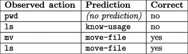
FIGURE 1.2 Example system performance.

Each of the metrics for this example are shown in Figure 1.3. To calculate precision, we see that three predictions were made and two of them were correct, giving us 66.7%. For recall, we note there were four possible prediction points (one after each observed action), and again, two correct predictions were made, giving us 50.0%.

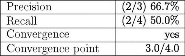
FIGURE 1.3 Evaluation metrics for example in Figure 1.2.

The example does converge since the last prediction was correct, therefore we can calculate a convergence point for it. After the third observed action, the recognizer made the right prediction, and it kept making this prediction throughout the rest of the plan session. Thus, we have a convergence point of 3.0 observed actions, over the total of 4.0 observed actions. Note that for a group of results, the denominator will be the average of total observed actions per each converged plan session.

1.4.2 Discussion

Plan recognition is almost never an end unto itself, but rather a component in a bigger system. However, this point is sometimes lost in the plan recognition field. It is important to use metrics beyond precision and recall to measure the behavior of systems to make sure that the systems we build can also handle early and partial predictions. Note that the general metrics described here do not cover partial prediction; however, we will introduce several metrics in the following for our formalism that do, by measuring performance at each level of the goal chain, as well as partial parameter prediction.

1.5 Hierarchical Goal Recognition

In this section, we discuss our system, which performs hierarchical recognition of both goal schemas and their parameters. We first describe the separate components: a goal schema recognizer and a goal parameter recognizer. We then discuss how these are put together to create a system that recognizes instantiated goals.

In most domains, goals are not monolithic entities; rather, they are goal schemas with instantiated parameters. Combining goal schema recognition with goal parameter recognition allows us to do instantiated goal recognition, which we will refer to here as simplygoal recognition.

First we give some definitions that will be useful throughout the chapter. We then describe the recognition model and our most recent results.

1.5.1 Definitions

For a domain, we define a set of goal schemas, each taking parameters, and a set of action schemas, each taking parameters. If actual goal and action schemas do not have the same number of parameters as the others, we can easily pad them with “dummy” parameters, which always take the same value.¹⁰

Given an instantiated goal or schema, it is convenient to refer to the schema of which it is an instance as well as each of its individual parameter values. We define a function that, for any instantiated action or goal, returns the corresponding schema. As a shorthand, we use , where is an instantiated action or goal.

To refer to parameter values, we define a function , which returns the value of the th parameter of an instantiated goal or action. As a shorthand, we use , where is again an instantiated action or goal.

As another shorthand, we refer to number sequences by their endpoints: . Thus, and .

1.5.2 Problem Formulation

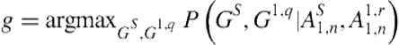
We define goal recognition as the following: given an observed sequence of instantiated actions observed thus far (), find the most likely instantiated goal :

(1.1)

If we expand the goal and actions into their schemas and parameters, this becomes¹¹:

(1.2)

If we assume that goal parameters are independent of each other and that goal schemas are independent from action parameters (given their action schemas), this becomes:

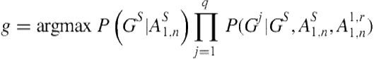(1.3)

In Equation (1.3), the first term describes the probability of the goal schema, , which we will use for goal schema recognition. The other terms describe the probability of each goal parameter, . We discuss these both in this section.

1.5.3 Goal Schema Recognition

1.5.3.1 Cascading Hidden Markov Models

In our hierarchical schema recognizer, we use a Cascading Hidden Markov Model (CHMM), which consists of stacked state-emission HMMs (). Each HMM () is defined by a 5-tuple , where is the set of possible hidden states; is the set of possible output states; is the initial state probability distribution; is the set of state transition probabilities; and is the set of output probabilities.

The HMMs are stacked such that for each HMM (), its output state is the hidden state of the HMM below it (). For the lowest level (), the output state is the actual observed output. In essence, at each timestep , we have a chain of hidden state variables () connected to a single observed output at the bottom level. An example of a CHMM is shown in Figure 1.4. Here, the th HMM (i.e., the HMM that starts with the hidden state () is a typical HMM with the output sequence . As we go up the CHMM, the hidden level becomes the output level for the level above it, and so forth.

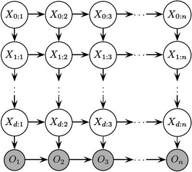
FIGURE 1.4 A Cascading Hidden Markov Model.

We will now describe the differences between CHMMs and other hierarchical HMMs. We then discuss how inference is done with CHMMs—in particular, how the forward probability is calculated, as this is a key part of our recognition algorithm.

Comparison to hierarchical HMMs

Hierarchical HMMs (HHMMs) [22] and the closely related Abstract HMMs (AHMMs) [12] also represent hierarchical information using a limited-depth stack of HMMs. In these models, an hidden state can output either a single observation or a string of observations. Each observation can also be associated with a hidden state at the next level down, which can also output observations, and so forth. In HHMMs, when a hidden state outputs an observation, control is transferred to that observation, which can also output and pass control. Control is only returned to the upper level (and the upper level moves to its next state) when the output observation has finished its output, which can take multiple timesteps.

In contrast, CHMMs are much simpler. Each hidden state can only output a single observation, thus keeping the HMMs at each level in lock-step. In other words, in CHMMs, each level transitions at each timestep, whereas only a subset transitions in HHMMs.

Next, we use CHMMs to represent an agent’s execution of a hierarchical plan. As we discuss there, mapping a hierarchical plan onto a CHMM results in a loss of information that could be retained by using an HHMM—compare to [12]. This, however, is exactly what allows us to do tractable online inference, as we show later. Exact reasoning in HHMMs has been shown to be exponential in the number of possible states [22].

Computing the forward probability in CHMMs

An analysis of the various kinds of inference possible with CHMMs is beyond the scope of this chapter. Here we only focus on the forward algorithm [28], which is used in our recognition algorithm.¹²

In a typical HMM, the forward probability () describes the probability of the sequence of outputs observed up until time () and that the current state is , given an HMM model (). The set of forward probabilities for a given timestep , (), can be efficiently computed using the forward algorithm, which uses a state lattice (over time) to efficiently compute the forward probability of all intermediate states. We describe the forward algorithm here to allow us to more easily show how it is augmented for CHMMs.

First, is initialized with initial state probabilities (). Then, for each subsequent timestep , individual forward probabilities are computed using the following formula:

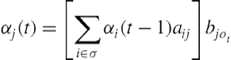(1.4)

The complexity of computing the forward probabilities for a sequence of observations is O (), where is the set of possible hidden states. However, as we will use the forward probability in making online predictions in the next section, we are more interested in the complexity for extending the forward probabilities to a new timestep (i.e., calculating given ). For extending to a new timestep, the runtime complexity is O (), or quadratic in the number of possible hidden states.

Algorithm overview

In a CHMM, we want to calculate the forward probabilities for each depth within a given timestep: , where . This can be done one timestep at a time, cascading results up from the lowest level ().

Initialization of each level occurs as normal—as if it were a normal HMM—using the start state probabilities in . For each new observation , the new forward probabilities for the chain are computed in a bottom-up fashion, starting with . At this bottom level, the new forward probabilities are computed as for a normal HMM using Eq. (1.4).

We then move up the chain, computing one forward probability set at a time, using the results of the level below as observed output. However, we cannot use Eq. (1.4) to calculate these forward probability sets () because the forward algorithm assumes that output is observed with certainty. While this was the case for level (where the output variable is ), for all other levels, the output state is actually also a hidden state (), and thus uncertain.

We overcome this by first observing that, although we do not know the value of with certainty, if we have the forward probability distribution for that node (), we can use it as a probability distribution over possible values for the state. As discussed before, we can compute the forward probability set at the bottom level , which gives us a probability distribution over possible values of . To calculate the forward probability at the next level up , as well as higher levels, we need to augment the forward algorithm to work for HMMs with uncertain output.

Changing the forward algorithm to handle uncertain output is straightforward, and needs only to include a weighted sum over output probabilities, as shown here:

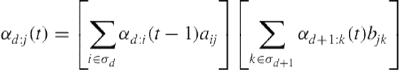(1.5)

Including this additional summation does not change the complexity of the forward algorithm. For updating each level, it remains quadratic in the number of hidden states .

1.5.3.2 Schema recognition algorithm

From the previous discussion, it may be quite apparent where we are going with this. A quick comparison of the goal chains in Figure 1.1 and the CHMM in Figure 1.4 shows a remarkable resemblance. Our hierarchical goal schema recognizer models an agent’s plan execution with a CHMM, with one level for each subgoal level in the hierarchical plan. The use of CHMMs requires having a plan tree of constant depth, which is not usually a valid assumption, including for the corpus we use later.

Given a variable depth corpus, we use a padding scheme to extend all leaves to the deepest level. To do this, we expand each leaf that is too shallow by copying the node that is its immediate parent and insert it between the parent and the leaf. We repeat this until the leaf node is at the proper depth. We refer to these copies of subgoals as ghost nodes.

After each observed action, predictions are made at each subgoal level using what we call augmented forward probabilities. Early experiments based purely on the CHMM forward probabilities gave only mediocre results. To improve performance, we added observation-level information to the calculations at each level by making both transition and output probabilities context-dependent on the current and last observed action (bigram). The idea was that this would tie upper-level predictions to possible signals present only in the actual actions executed, as opposed to just some higher-level, generic subgoal. This is similar to what is done in probabilistic parsing [15], where lexical items are included in production probabilities to provide better context.

The only change we made was to the transition probabilities () and output probabilities () at each level. Thus, instead of the transition probability being , we expand it to be conditioned on the observed actions as well:

Similarly, we added bigram information to the output probabilities ():

We will now describe how the CHMM is trained, and then how predictions are made. We then analyze the runtime complexity of the recognition algorithm.

Training the CHMM

As a CHMM is really just a stack of HMMs, we need only to estimate the transition probabilities (), output probabilities (), and start state probabilities () for each depth . To estimate these, we need a plan-labeled corpus (as described before) that has a set of goals and associated plans. Each hierarchical plan in the corpus can be converted into a set of goal chains, which are used to estimate the different probability distributions.

Predictions

At the start of a recognition session, a CHMM for the domain is initialized with start state probabilities from the model. After observing a new action, we calculate the new forward probabilities for each depth using the CHMM forward algorithm.

Using the forward probabilities, n-best predictions are made separately for each level. The most likely schemas are chosen, and their combined probability is compared against a confidence threshold . If the n-best probability is greater than , a prediction is made. Otherwise, the recognizer does not predict at that level for that timestep.

It is important to note that using this prediction algorithm means it is possible that, for a given timestep, subgoal schemas may not be predicted at all depths. It is even possible (and actually occurs in our experiments that follow) that the depths at which predictions occur can be discontinuous (i.e., a prediction could occur at levels 4, 3, and 1, but not 2 or 0). We believe this to be a valuable feature because subgoals at different levels may be more certain than others.

Complexity

The runtime complexity of the recognizer for each new observed timestep is the same as that of forward probability extension in the CHMM: , where is depth of the deepest possible goal chain in the domain (not including the observed action), and is the set of possible subgoals (at any level). Thus, the algorithm is linear in the depth of the domain and quadratic in the number of possible subgoals in the domain.

1.5.4 Adding Parameter Recognition

The preceding system only recognizes goal schemas. To do full goal recognition, we also need to recognize the parameter values for each posited goal schema. Put more precisely, for each recognized goal schema, we need to recognize the value for each of its parameter slots.

First briefly describe the top-level parameter recognition algorithm and then describe how it can be augmented to support parameter recognition within a hierarchical instantiated goal recognizer.

1.5.4.1 Top-level parameter recognition

One straightforward way of doing parameter recognition would be to treat instantiated goal schemas as atomic goals and then use the goal schema recognition algorithm. However, this solution has several problems. First, it would result in an exponential increase in the number of goals, as we would have to consider all possible ground instances. This would seriously impact the speed of the algorithm. It would also affect data sparseness, as the likelihood of seeing an n-gram in the training data will decrease substantially.

Instead, we perform goal schema and parameter recognition separately, as described in Equation (1.3). From the last term of the equation, we get the following for a single parameter :

(1.6)

We could estimate this with an n-gram assumption, as we did before. However, there are several problems here as well.

First, this would make updates at least linear in the number of objects in the world (the domain of ), which may be expensive in domains with many objects. Second, even without a large object space, we may run into data sparsity problems, since we are including both the action schemas and their parameter values.

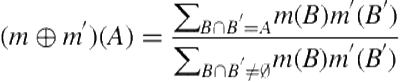
This solution misses out on the generalization that, often, the positions of parameters are more important than their value. For example, in a Linux goal domain, the first parameter (i.e., the source file) of the action mv is often the $filename parameter of a goal to move a file of a certain name, whereas the second parameter (i.e., the destination) almost never is, regardless of the parameter’s actual value. Our model learns probability distributions of equality over goal and action parameter positions. During recognition, we use these distributions along with a special, tractable case of Dempster-Shafer Theory to dynamically create a set of possible parameter values and our confidence in them, which we use to estimate Equation (1.6).

Formally, we want to learn the following probability distribution: . This gives us the probability that the value of the th parameter of action is equal to the th parameter of the goal , given both the goal and action schemas as well as the two parameter positions. Note that the value of the parameter is not considered here, only the position. We can easily compute this conditional probability distribution from the training corpus.

To use this model to predict the value of each goal schema parameter as we make action observations, we need to be able to combine probabilities for each parameter in the observed action, as well as probabilities from action to action. For this we use the Dempster-Shafer Theory.

Dempster-Shafer Theory

Dempster-Shafer Theory (DST) [30] is a generalization of probability theory that allows for incomplete knowledge. Given a domain , a probability mass is assigned to each subset of , as opposed to each element, as in classical probability theory. Such an assignment is called a basic probability assignment (bpa).

Assigning a probability mass to a subset in a bpa means that we place that level of confidence in the subset but cannot be any more specific. For example, suppose we are considering the outcome of a die roll ().¹³ If we have no information, we have a bpa of (i.e., all our probability mass is on ). This is because, although we have no information, we are 100% certain that one of the elements in is the right answer; we just cannot be more specific.

Now suppose we are told that the answer is an even number. In this case, our bpa would be ; we have more information, but we still cannot distinguish between the even numbers. A bpa of and would intuitively mean that there is a 50% chance that the number is even, and a 50% chance that it is 1. The subsets of that are assigned nonzero probability mass are called the focal elements of the bpa.

A problem with DST is that the number of possible focal elements of is the number of its subsets, or . This is both a problem for storage and for time for bpa combination (as discussed later). For parameter recognition, we use a special case of DST that only allows focal elements to be singleton sets or (the entire set). This, of course, means that the maximum number of focal elements is . As we show in the following, this significantly decreases the complexity of a bpa combination, allowing us to run in time linear with the number of actions observed so far, regardless of the number of objects in the domain.

Evidence combination

Two bpas, and , representing different evidence can be combined into a new bpa using Dempster’s rule of combination:

(1.7)

The complexity of computing this is , where and are the number of focal elements in and , respectively. Basically, the algorithm does a set intersection (hence the term) for combinations of focal elements.

As mentioned earlier, the complexity would be prohibitive if we allowed any subset of to be a focal element. However, our special case of DST limits and to . Also, because we only deal with singleton sets and , we can do set intersections in constant time. Thus, for our special case of DST, the complexity of Dempster’s rule of combination becomes , or in the worst case.

As a final note, it can be easily shown that our special case of DST is closed under Dempster’s rule of combination. We omit a formal proof, but it basically follows from the fact that the set intersection of any two arbitrary focal-element subsets from special-case bpas can only result in —a singleton set, or the empty set. Thus, as we continue to combine evidence, we are guaranteed to still have a special-case bpa.

Representing the model with DST

As stated before, we estimate from the corpus. For a given goal schema and the th action schema , we define a local bpa for each goal and action parameter positions and s.t. and . This local bpa intuitively describes the evidence of a single goal parameter value from looking at just one parameter position in just one observed action. The bpa has two focal elements: , which is a singleton set of the actual action parameter value, and . The probability mass of the singleton set describes our confidence that this value is the goal parameter value. The probability mass of expresses our ignorance, as it did in the preceding die roll example.

To smooth the distribution, we always make sure that both elements ( and ) are given at least a little probability mass. If either one is 1, a very small value is taken from that and given to the other. Several things are worth noting here.

First, we assume here that we already know the goal schema . This basically means that we have a two-step process with which we first recognize the goal schema and then use that to recognize the parameters. The following discusses how we can combine these processes in a more intelligent way.

Second, if a goal schema has more than one parameter, we keep track of these and make predictions about them separately. As we discuss next, it is possible that we will be more confident about one parameter and predict it, whereas we may not predict another parameter for the same goal schema. This allows us to make more fine-grained partial predictions. Finally, we do not need to represent, enumerate, or even know the elements of . This means that we can handle domains where the set of possible values is very large, or in which values can be created or destroyed.

Combining evidence

As mentioned earlier, we maintain a separate prediction bpa for each goal parameter position . Each of these are initialized as , which indicates complete ignorance about the parameter values. As we observe actions, we combine evidence within a single action and then among single actions.

First, within a single action , we combine each of the local bpas for each parameter position , which gives us an action bpa . This describes the evidence the entire action has given us. Then, we combine the evidence from each observed action to give us an overall prediction bpa that describes our confidence in goal parameter values given all observed actions so far. We then use this prediction bpa to make (or not make) predictions. When we observe an action , we create local bpas for each action parameter position . The action bpa is the combination of all these: . The prediction bpa is similarly calculated from all action bpas from observed actions: . However, we can calculate this incrementally by calculating at each action observation. This allows us to only do 1 action–bpa combination per observed action.

It is worth noting here that only values that we have seen as action parameter values will be part of the prediction bpa. Thus, the maximum number of focal elements for a bpa will be the total number of unique action parameters seen, plus 1 (for ). As a corollary, this means that our method will not be able to correctly predict a goal parameter unless its value has been seen as an action parameter value during the current plan session.

In what follows, we report results of total recall and also “recall/feasible,” which restricts recall to the prediction points at which the algorithm had access to the right answer. Admittedly, there are domains in which the correct parameter value could be learned directly from the training corpus without having been seen in the current session, although we do not believe it will be so in most cases.

Prediction

At some level, we are using the prediction bpa as an estimation of from Equation (1.6). However, because the bpa contains , it is not a true probability distribution and cannot provide a direct estimation. Instead, we use as a measure of confidence in deciding whether to make a prediction.

To make an -best prediction, we take the singleton sets with the highest probability mass and compare their combined mass with that of . If their mass is greater, we make that prediction. If has a greater mass, we are still too ignorant about the parameter value and hence therefore make no prediction.

Complexity

The other thing to mention is the computational complexity of updating the prediction bpa for a single goal parameter . We first describe the complexity of computing the th action bpa and then the complexity of combining it with the previous prediction bpa .

To compute , we combine 2-focal-element local bpas, one for each action parameter position. If we do a serial combination of the local bpas (i.e., ), this results in combinations, where the first bpa is an intermediate composite bpa and the second is always a 2-element local bpa. Each combination (maximally) adds just 1 subset to (the other subset is which is always shared). The ()th combination result will have maximum length . The combination of that with a local bpa is (). Thus, the overall complexity of the combination of the action bpa is .

The action bpa is then combined with the previous prediction bpa, which has a maximum size of (i.e., from the number of possible unique action parameter values seen). The combination of the two bpas is , which, together with the complexity of the computation of the action bpa, becomes . Here, is actually constant (and should be reasonably small), so we can treat it as a constant, in which case we get a complexity of . This is done for each of the goal parameters, but is also constant, so we still have . This gives us a fast parameter recognition algorithm that is not dependent on the number of objects in the domain.

1.5.4.2 Hierarchical parameter recognition

Application of this parameter recognition algorithm to the hierarchical case is not straightforward. For the rest of this section, we first describe our basic approach to hierarchical instantiated goal recognition and then discuss several problems (and their solutions) with incorporating the parameter recognizer.

The basic algorithm of the hierarchical instantiated goal recognizer is as follows: After observing a new action, we first run the hierarchical schema recognizer and use it to make preliminary predictions at each subgoal level. At each subgoal level, we associate a set of parameter recognizers, one for each possible goal schema, which are then updated in parallel. This is necessary because each parameter recognizer is predicated on a particular goal schema. Each parameter recognizer is then updated by the process described next to give a new prediction bpa for each goal parameter position. If the schema recognizer makes a prediction at that level (i.e., its prediction was above the threshold ), we then use the parameter recognizers for the predicted goal schemas to predict parameter values in the same way just described. This is similar to the algorithm used by our instantiated top-level goal recognizer [9], and it combines the partial prediction capabilities of the schema and parameter recognizers to yield an instantiated goal recognizer.

Dealing with uncertain output

One problem when moving the parameter recognizer from a “flat” to a hierarchical setting is that, at higher subgoal levels, the hidden state (subgoal predictions) of the level below becomes the output action. This has two consequences: first, instead of the output being a single goal schema, it is now a probability distribution over possible goal schemas (computed by the schema recognizer at the lower level). Second, instead of having a single parameter value for each subgoal parameter position, we now have the prediction bpa from the parameter recognizer at the level below.

We solve both of these problems by weighting evidence by its associated probability. In general, a bpa in DST can be weighted using Wu’s weighting formula [31]:

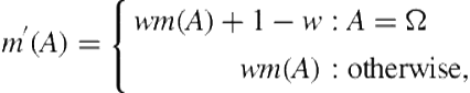(1.8)

where is the bpa to be weighted and is the weight. This equation essentially weights each of the focal points of the bpa and redistributes lost probability to , or the ignorance measure of the bpa.

To handle uncertain parameter values in the output level, we change the computation of local bpas. Here, we have an advantage because the uncertainty of parameter values at the lower level is actually itself represented as a bpa (the prediction bpa of the parameter recognizer at the lower level). We compute the local bpa by weighting that prediction bpa with the probability of positional equality computed from the corpus ().

Using these local bpas, we can then calculate the action bpa (or evidence from a single action or subgoal) in the same way as the original parameter recognizer. However, we still have the lingering problem of having uncertain subgoal schemas at that level. Modifying the updated algorithm for this case follows the same principle we used in handling uncertain parameters.

To handle uncertain goal schemas, we compute an action bpa for each possible goal schema. We then introduce a new intermediate result called an observation bpa, which represents the evidence for a parameter position given an entire observation (i.e., a set of uncertain goal schemas each associated with uncertain parameter values). To compute the observation bpa, first each action bpa in the observation is weighted according to the probability of its goal schema (using Eq. (1.8)). The observation bpa is then computed as the combination of all action bpas. This effectively weights the contributed evidence of each uncertain goal schema according to its probability (as computed by the schema recognizer).

Uncertain transitions at the prediction level

In the original parameter recognizer, we assumed that the agent only had a single goal that needed to be recognized, thus we could assume that the evidence we saw was always for the same set of parameter values. However, in hierarchical recognition this is not the case because subgoals may change at arbitrary times throughout the observations (refer to Figure 1.1).

This is a problem because we need to separate evidence. In the example shown in Figure 1.1, subgoals and give us evidence for the parameter values of but presumably not (directly) . Ideally, if we knew the start and end times of each subgoal, we could simply reset the prediction bpas in the parameter recognizers at that level after the third observation when the subgoal switched.

In hierarchical recognition, we do not know a priori when goal schemas begin or end. We can, however, provide a rough estimation by using the transition probabilities estimated for each HMM in the schema recognizer. We use this probability (i.e., the probability that a new schema does not begin at this timestep) to weight the prediction bpa at each new timestep.

Basically, this provides a type of decay function for evidence gathered from previous timesteps. Assuming we could perfectly predict schema start times, if a new schema started, we would have a 0 probability; thus, weighting would result in a reset prediction bpa. On the other hand, if a new subgoal did not start, then we would have a weight of 1 and thus use the evidence as it stands.

Uncertain transitions at the output level

A more subtle problem arises from the fact that subgoals at the output level may correspond to more than one timestep. As an example, consider again the goal chain sequence in Figure 1.1. At level 2, the subgoal is output for two timesteps by . This becomes a problem because Dempster’s rule of combination makes the assumption that combined evidence bpas represent independent observations. For the case in Figure 1.1, when predicting parameters for , we would combine output evidence from two separate times (as two separate observation bpas), as if two separate events had occurred.

The predictions for , of course, will likely be different at each of the timesteps, reflecting the progression of the recognizer at that level. However, instead of being two independent events, they actually reflect two estimates of the same event, with the last estimate presumably being the most accurate (because it has considered more evidence at the output level).

To reflect this, we also change the update algorithm to keep track of the prediction bpa formed with evidence from the last timestep of the most recently ended subgoal at the level below; this we call the last subgoal prediction (lsp) bpa. At a new timestep, the prediction bpa is formed by combining the observation bpa with this lsp bpa. If we knew the start and end times of subgoals, we could simply discard this prediction bpa if a subgoal had not yet ended, or make it the new lsp if it had. Not knowing schema start and end times gives us a similar problem at the output level. As we discussed, we need a way of distinguishing which observed output represents a new event versus which represents an updated view of the same event.

We handle this case in a similar way to that mentioned before. We calculate the probability that the new observation starts a new timestep by the weighted sum of all same transition probabilities at the level below. This estimate is then used to weight the prediction bpa from the last timestep and then combine it with the lsp bpa to form a new lsp bpa. In cases in which there is a high probability that a new subgoal was begun, the prediction bpa will have a large contribution to the lsp bpa, whereas it will not if the probability is low.

Complexity

First, we must analyze the complexity of the modified parameter recognizer, which deals with output with uncertain goal schemas. In this analysis, is the number of possible goal schemas, is the maximum parameters for a goal schema, is the current timestep, and is the depth of the hierarchical plan.

The modified algorithm computes the observation bpa by combining (worst case) action bpas—each with a maximum size of . Thus, the total complexity for the update of a single parameter position is ; for the parameter recognizer of a single goal schema (with parameter positions), this becomes . As is constant and likely small, we drop it, which gives us .

The complexity of an update for the instantiated recognizer can be calculated from the runtime of the schema recognizer plus the runtime of each of the parameter recognizers (one per each goal schema per level). Thus, the total runtime complexity is , or quadratic in the number of possible goal schemas and the number of actions observed so far.

1.6 System Evaluation

We now report on our experiments: first on the parameter recognizer itself, and then on the hierarchical instantiated goal recognizer. For the experiments, we used 4500 plan sessions from the Monroe Plan Corpus (described earlier and in [8]) for training and the remaining 500 for testing. This is the same data used in the experiments on our instantiated top-goal recognizer [9] and allows us to make comparisons.

Before we describe the experiments and their results, however, we briefly discuss the metrics we use to report results.

1.6.1 Metrics

We report results for individual subgoal depths, as well as totals. For each depth, we use the same metrics described previously.

In reporting results for each level (and in the total), we do not count predictions when the correct answer was a “ghost” node; they, as we described, are used to pad the plan tree such that all leaves are at the same depth. Ghost node prediction tends to be correct, and thus resulted in heavily inflated results, especially at lower depths. Ghost nodes were only introduced to support use of CHMMs, so it is unfair to credit these as correct predictions.

In reporting results for parameter recognition, we additionally use recall/feasible and convergence/feasible, which measure recall and convergence for those cases in which it was possible for the parameter recognizer to get the right answer. As described earlier, our algorithm for parameter recognition can never predict a parameter that has not yet been seen as the parameter of an observed action.

In reporting results for instantiated recognition, Parameter Percentage reports, for all correct predictions, the percentage of the goal parameters that were predicted. Convergence Parameter Percentage reports the same for all sessions that converged. These are an attempt to measure the specificity of correct predictions made. For hierarchical recognition, we make a change to how convergence and convergence point are calculated. Some subgoals only span one timestep (e.g., they only result in one executed atomic action); in this case, it does not make sense to report convergence or a convergence point. For all levels, we only report convergence and convergence point for subgoals that correspond to at least two timesteps.

1.6.2 Schema Recognition Results

The results of the experiment are shown in Table 1.2. Overall, the results are very encouraging with 81.9% precision and 52.3% recall for 1-best prediction, which jumps to 94.9% precision and 71.4% recall for 2-best prediction. In the 2-best case, 95.7% of sessions converged on the right answer. On average, this was after a little more than half of the actions had been observed.

Table 1.2

Results of the Hierarchical Schema Recognition Experiment

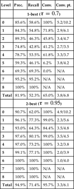
We now discuss the various levels in detail, first looking at the results for predicting top-level goal schemas (level 0) and then the other levels.

1.6.2.1 Top-level results

Results at the top level are also encouraging with 85.6% precision and 58.6% recall for 1-best prediction and 90.7% precision and 62.0% recall for 2-best. For comparison, we present the results of our top-level recognizer on the same dataset in Table 1.3.

Table 1.3

Results of Top-level Goal Schema Recognition

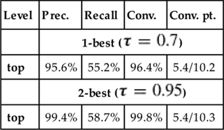
For recall, convergence, and convergence point, the two recognizers’ performance is fairly equivalent, both in 1-best and 2-best predictions. Precision, however, is markedly lower in the hierarchical recognizer for both the 1-best and 2-best cases. Whereas precision is 95.6% for 1-best in the flat recognizer, it drops to 85.7% for the hierarchical recognizer. A similar drop in precision from 99.4% to 91.5% is shown in the 2-best case.

Although there seem to be several factors involved in this drop, it is perhaps most important to mention two. First is the loss of true bigram information within the hierarchical recognizer. In the hierarchical recognizer, the top-level goal is predicted based on predictions at the next immediate subgoal level (level 1) as opposed to directly from the action observation level as is the top-level goal recognizer. Converting a plan tree into a sequence of goal chains loses explicit information about the actual previous subgoal.

Second, and most important, a direct comparison of algorithm performance is difficult because the hierarchical recognizer is doing much more than simple top-level goal classification, as was done in the top-level goal recognizer. Arguably, we could improve performance by using the hierarchical recognizer for the subgoal levels and then the flat recognizer for top-level recognition, although this then loses the generalization that the hierarchical recognizer can also handle cases where several top-level goals are pursued serially.

1.6.2.2 Other levels

Results at lower levels for 1-best prediction are on average not as good as those at the top level. The main reason is that there is actually more competition at lower levels, where more subgoals are possible, whereas only the 10 top-level schemas are possible at level 0. Also, there are several lower-level subgoals per level throughout a goal session. Only one top-level goal makes the transition probabilities much simpler at the top level as well; basically, transition probabilities are 1 between the same schemas and 0 between any others. This seems to especially account for the very low convergence numbers for levels 5 and 6 (6.2% and 0.0%, respectively), where there were only a few data points and these were fully recognized at the start of their interval, but not at the end. (In 2-best prediction both of these move to 100% convergence.)

That said, in the 1-best case, recognition results are fairly good for levels 1, 2, 7, and 8, although there is a trough between them. A partial explanation is that, at higher levels, there are less competitors. Thus, as we move to lower levels, things become more difficult to predict. At the same time, the lower we go, the closer to the observed output, and therefore the closer to certain information. Thus, the last two levels have very good precision and recall because they are so closely related to the observed action. (Levels 7 and 8 contained no subgoals that span more than one timestep, hence convergence and convergence point are not reported.)

It appears that in the middle (e.g., levels 3–6), the recognizer tends to not distinguish well among close competitors. That this is the case can be shown by looking at the 2-best case, where all levels move to the 90s or 100% for precision and also improve dramatically in recall.

1.6.3 Parameter Recognition Results

To test the parameter recognizer in its own right, we assumed perfect schema recognition—that is, for each new observation, we gave the parameter recognizer information about the chain of goal schemas at that time point, including information about which schemas began at that timestep. This perfect information about schema transitions meant that the parameter recognizer did not need to deal with (1) uncertain transitions at the prediction level and (2) uncertain schemas at the output level. Note that there was still uncertainty at the output level at higher levels because parameter values were still potentially uncertain, even though the schema was known (see Table 1.4).

Table 1.4

Results of Parameter Recognition

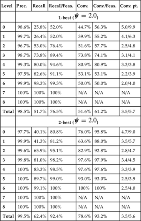
1.6.3.1 Top-level results

To help interpret the results, we compare performance at the top level to that of the flat recognizer, which only made predictions at the top level. For convenience, the results of the flat parameter recognizer on the same dataset are shown in Table 1.5. The hierarchical parameter recognizer performed slightly better in both the 1-best and 2-best cases. In 1-best, precision moved from 94.3% to 98.6%, although there was a drop in recall from 27.8% to 25.8%. In the 2-best recognizer, results were slightly better all around (see Table 1.6).

Table 1.5

Results of Flat Parameter Recognition

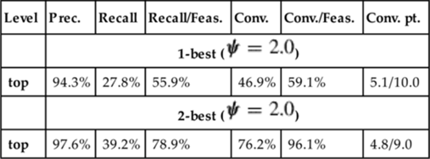
Table 1.6

Results of Instantiated Recognition

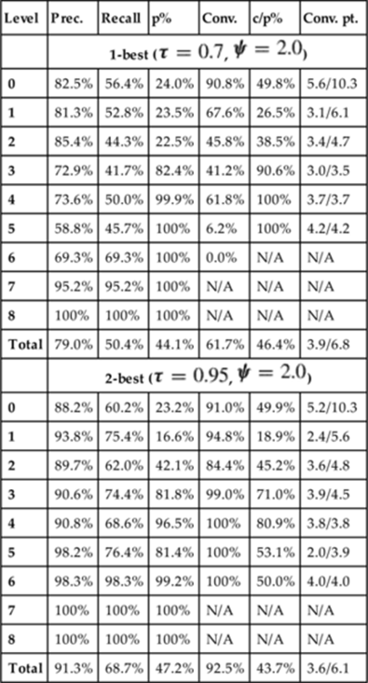
The reason for the improvement in performance is likely attributable to the fact that (perfect) subgoal schema information was present in the hierarchical recognizer. This allowed parameter values to be considered given the immediate child subgoal, giving better context for predictions.

1.6.3.2 Other levels

The hierarchical parameter recognizer performed well at other levels too, with precision staying (for the 1-best case) in the high 90s and even up to 100% for levels 7 and 8. This performance inched up for the 2-best case (with 100% precision for levels 4–8).

It is interesting to note that recall begins quite low (25.8% for level 0) and then climbs as we go down levels, reaching 100% for levels 7 and 8. As mentioned earlier, high absolute recall is not to be expected in plan recognition, as ambiguity is almost always present. The closer we move to the actual observed action, however, the higher precision gets. This can be attributed to two factors.

First, subgoals at lower levels are closer to the observed input, and thus deal with less uncertainty about what the parameter values are. Second, and probably most important, lower-level subgoals span fewer timesteps than those at higher levels, meaning that, if parameter values are available, they will be seen after a shorter number of actions.

In the case of levels 7 and 8, all subgoals only spanned one timestep, and thus only had one chance to get the right parameter values. It turns out that parameter values at these levels always directly corresponded to the action parameters, which is why precision and recall reach 100% here.

Overall, the performance of the parameter recognizer was very encouraging, especially the performance at lower levels that had high recall. This is an important factor in our ability to do specific and accurate partial prediction in the instantiated goal recognizer, which we move to now.

1.6.4 Instantiated Recognition Results

Here we examine the results of experiments on the instantiated hierarchical goal recognizer, which combined both schema and parameter recognizers as described previously. We first look at the results at the top level (i.e., level 0) and then the other levels.

1.6.4.1 Top-level results

To help interpret the results, we compare performance at the top level to that of our “flat” goal recognizer, which only made predictions at the top level. For convenience, the results of the flat instantiated recognizer on the same dataset are shown in Table 1.7.

Table 1.7

Results of Flat Instantiated Recognition on the Monroe Corpus

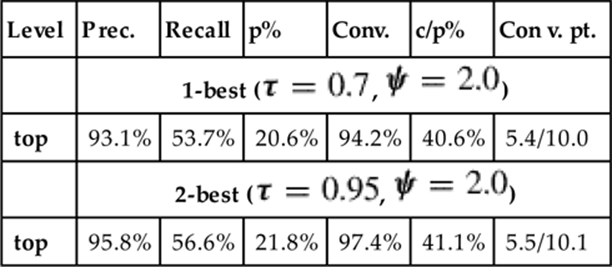
Note: Compare to [9].

Hierarchical instantiated results at the top level closely mirror results of the hierarchical schema recognizer [9]. This also happened for the flat recognizer and is to be expected, as schema recognition performance limits performance of the instantiated recognizers. The addition of parameter predictions serves to degrade the precision and recall of schema recognition results.

In the 2-best case, precision decreased from 95.8% in the flat recognizer to 88.2% in the hierarchical recognizer. However, recall increased from 56.6% to 60.2% and parameter percentage from 21.8% to 23.2%. This difference was more stark in convergence parameter percentage, which rose from 41.1% to 49.9%.

Although moving to a hierarchical recognizer seemed to degrade performance at the top level, at least in precision, this may be somewhat misleading because of the relative short length 9.5 actions of plans in the Monroe domain. We believe that longer, more complex plans will make it much more difficult to predict the top-level goal early on, thus requiring partial recognition of subgoals. Of course, this remains to be tested.

1.6.5 Other Levels

Precision and recall at other levels also closely mirror the performance of the schema recognizer. Precision dips in the middle levels but levels out for 2-best prediction, which achieves precision ranging from the high 80s to 100% (with recall ranging in the 60s and 70s for high levels and high 90s and 100% for the lower levels).

For 1-best parameter prediction for levels 1 and 2, it remains in the 20s, with a sudden jump to 82.4% at level 3, 99.9% at level 4, and 100% for the lower levels. Note that the drop in parameter prediction at several levels in the 2-best case is a result of the fact that the recognizer gets more cases right (i.e., increases recall), but that many of the new correct predictions have less instantiated parameter values. Thus, the decrease in number reflects that the recognizer is getting more correct predictions, but it does not reflect a decrease in performance for the cases it got correct in the 1-best prediction.

1.7 Conclusion

In this chapter, we have formalized hierarchical goal recognition as the recognition of the chain of an agent’s active subgoals given an observed action. We discussed needed metrics and data for plan recognition, and introduced a method for creating synthetic plan-labeled corpora using a randomized AI planner and Monte Carlo sampling, which was used to create the Monroe Plan Corpus. We also described a hierarchical goal recognition system that is able to recognize goal schemas and their parameters. We then showed its performance on the Monroe Plan Corpus.

We believe that an important area of future research will be the generalization of plan recognition to what we will call problem-solving recognition. Plan recognition is typically defined as the recognition of an agent’s plan, given observed actions. This definition, however, implicitly makes the assumption that an agent first creates a plan and then executes it.

Of course this is not always the case, and we would argue that there are many domains in which this is usually not the case. We believe if we want to model real agents from observations, we need to recognize the agent’s problem-solving activity itself. This would mean recognizing the agent’s current problem-solving state, which could then change from timestep to timestep. There would no longer be a single plan data object attached to a plan session; rather, a post hoc view of a plan session would reveal a trace of the agent’s problem-solving state over the session.

The agent may have had several (partial or full) plans over the session, which may have been expanded or revised (or scrapped) as time passed. This would also model shifts in execution of different plans for different objectives, and even phenomena such as goal abandonment. (It could be very useful to know when an agent has abandoned a goal without accomplishing it.) See Geib and Goldman [17] as an example of work on recognizing plan abandonment.

As this is a very new area, much work is needed here. However, as a possible extension to our work, we have considered the possibility of using an artificial agent to create a problem-solving labeled corpus which could then not only give us information about hierarchical goal structure over time but also could be used to train a recognizer to predict when phenomena (e.g., replanning or goal abandonment) has occurred. See Oliver et al. [24] for an example of using an agent to create synthetic data.

References

1. Albrecht DW, Zukerman I, Nicholson AE. Bayesian models for keyhole plan recognition in an adventure game. User Model User-Adapted Interact. 1998;8:5-47.

2. Ashbrook D, Starner T. Using GPS to learn significant locations and predict movement across multiple users. Personal Ubiquitous Comput. 2003;7(5):275-286.

3. Bauer M. A Dempster-Shafer approach to modeling agent preferences for plan recognition. User Model User-Adapted Interact. 1995;5:3-4.

4. Bauer M. Acquisition of user preferences for plan recognition. Proceedings of the Fifth International Conference on User Modeling. 1996:105-112.

5. Bauer M. Acquisition of abstract plan descriptions for plan recognition. Proceedings of the 15th National Conference on Artificial Intelligence. 1998:936-941.

6. Bauer M, Paul G. Logic-based plan recognition for intelligent help systems. In: Bäckström C, Sandewall E, editors. Current trends in AI planning. EWSP ’93—Second European workshop on planning. Frontiers in artificial intelligence and applications; 1993. p. 60–73 [see also DFKI Research, Report RR-93-43].

7. Blaylock N, Allen J. Statistical goal parameter recognition. In: Zilberstein S, Koehler J, Koenig S, eds. Proceedings of the 14th International Conference on Automated Planning and Scheduling. 2004:297-304.

8. Blaylock N, Allen J. Generating artificial corpora for plan recognition. In: Ardissono L, Brna P, Mitrovic A, eds. User Modeling. Springer; 2005:179-188.

9. Blaylock N, Allen J. Recognizing instantiated goals using statistical methods. In: Kaminka G, editor. IJCAI workshop on modeling others from observations; 2005b. p. 79–86.

10. Bui HH. Efficient approximate inference for online probabilistic plan recognition. Tech. Rep. 1/2002, School of Computing, Curtin University of Technology; 2002.

11. Bui HH. A general model for online probabilistic plan recognition. In: Gottlob G, Walsh T, eds. Proceedings of the 18th International Joint Conference on Artificial Intelligence. 2003.

12. Bui HH, Venkatesh S, West G. Policy recognition in the abstract hidden Markov model. J Artif Intell Res. 2002;17.

13. Carberry S. Plan recognition in natural language dialogue (ACL-MIT Press series on natural language processing). MIT Press; 1990.

14. Carberry S. Techniques for plan recognition. User Model User-Adapted Interact. 2001;11:31-48.

15. Charniak E. Statistical techniques for natural language parsing. AI Mag. 1997;18(4):33-43.

16. Davison BD, Hirsh H. Predicting sequences of user actions. In: Notes of the AAAI/ICML. Workshop on predicting the future: AI approaches to time-series analysis; 1998. p. 5–12.

17. Geib CW, Goldman RP. Recognizing plan/goal abandonment. In: Gottlob G, Walsh T, eds. Proceedings of the 18th International Joint Conference on Artificial Intelligence. 2003:1515-1517.

18. Horvitz E, Paek T. A computational architecture for conversation. Proceedings of the Seventh International Conference on User Modeling. 1999:201-210.

19. Lesh N. Scalable and adaptive goal recognition. Ph.D. thesis, University of Washington; 1998.

20. Lesh N, Rich C, Sidner CL. Using plan recognition in human-computer collaboration. In: Proceedings of the Seventh International Conference on User Modeling; 1999 [see also MERL Technical, Report TR98-23].

21. Mitchell TM, Wang SH, Huang Y, Cheyer A. Extracting knowledge about users’ activities from raw workstation contents. Proceedings of the 21st National Conference on Artificial Intelligence. 2006:181-186.

22. Murphy KP, Paskin MA. Linear time inference in hierarchical HMMs. Proceedings of Neural Information Processing Systems. 2001:833-840.

23. Nau D, Au T-C, Ilghami O, Kuter U, Murdock JW, Wu D, et al. SHOP2: an HTN planning system. J Artif Intell Res. 2003;20:379-404.

24. Oliver NM, Rosario B, Pentland A. Graphical models for recognizing human interactions. Proceedings of International Conference on Neural Information and Processing Systems. 1998:924-930.

25. Patterson DJ, Liao L, Fox D, Kautz H. Inferring high-level behavior from low-level sensors. Fifth Annual Conference on Ubiquitous Computing. 2003.

26. Pynadath DV, Wellman MP. Accounting for context in plan recognition, with application to traffic monitoring. Proceedings of the 11th Conference on Uncertainty in Artificial Intelligence. 1995:472-481.

27. Pynadath DV, Wellman MP. Probabilistic state-dependent grammars for plan recognition. Proceedings of the 16th Conference on Uncertainty in Artificial Intelligence. 2000.

28. Russell S, Norvig P. Artificial intelligence: a modern approach. 2nd ed. Pearson Education; 2003.

29. Sadilek A, Kautz H. Location-based reasoning about complex multi-agent behavior. J Artif Intell Res. 2012;43:87-133.

30. Shafer G. A mathematical theory of evidence. Princeton University Press; 1976.

31. Wu H. Sensor data fusion for context-aware computing using Dempster-Shafer theory. Ph.D. thesis, Carnegie-Mellon University, Robotics Institute; 2003.