Algorithms Third Edition in C++ Part 5. Graph Algorithms (2006)
CHAPTER EIGHTEEN
Graph Search
18.3 Graph-Search ADT Functions
DFS and the other graph-search methods that we consider later in this chapter all involve following graph edges from vertex to vertex, with the goal of systematically visiting every vertex and every edge in the graph. But following graph edges from vertex to vertex can lead us to all the vertices in only the same connected component as the starting vertex. In general, of course, graphs might not be connected, so we need one call on a search function for each connected component. We
Program 18.2 Graph search
This base class is for processing graphs that may not be connected. Derived classes must define a function searchC that, when called with a self-loop to v as its second argument, sets ord[t]to cnt++ for each vertex t in the same connected component as v. Typically, constructors in derived classes call search, which calls searchC once for each connected component in the graph.
template <class Graph> class SEARCH
{
protected:
const Graph &G;
int cnt;
vector <int> ord;
virtual void searchC(Edge) = 0;
void search()
{ for (int v = 0; v < G.V(); v++)
if (ord[v] == -1) searchC(Edge(v, v)); }
public:
SEARCH (const Graph &G) : G(G),
ord(G.V(), -1), cnt(0) { }
int operator[](int v) const { return ord[v]; }
};
will typically use graph-search functions that perform the following steps until all of the vertices of the graph have been marked as having been visited:
• Find an unmarked vertex (a start vertex).
• Visit (and mark as visited) all the vertices in the connected component that contains the start vertex.
The method for marking vertices is not specified in this description, but we most often use the same method that we used for the DFS implementations in Section 18.2: We initialize all entries in a private vertex-indexed vector to a negative integer, and mark vertices by setting their corresponding entry to a nonnegative value. Using this procedure amounts to using a single bit (the sign bit) for the mark; most implementations are also concerned with keeping other information associated with marked vertices in the vector (such as, for the DFS implementation in Section 18.2, the order in which vertices are marked). The method for looking for a vertex in the next connected component is also not specified, but we most often use a scan through the vector in order of increasing index.
We pass an edge to the search function (using a dummy self-loop in the first call for each connected component), instead of passing its destination vertex, because the edge tells us how we reached the vertex. Knowing the edge corresponds to knowing which passage led to a particular intersection in a maze. This information is useful in many DFS classes. When we are simply keeping track of which vertices we have visited, this information is of little consequence; but more interesting problems require that we always know from whence we came.
Program 18.2 is an implementation that illustrates these choices. Figure 18.8 gives an example that illustrates how every vertex is visited, by the effect on the ord vector of any derived class. Typically, the derived classes that we consider also examine all edges incident upon each vertex visited. In such cases, knowing that we visit all vertices tells us that we visit all edges as well, as in Trémaux traversal.
Program 18.3 is an example that shows how we derive a DFS-based class for computing a spanning forest from the SEARCH base class of Program 18.2. We include a private vector st in the derived class to hold a parent-link representation of the tree that we initialize in the constructor; define a searchC that is similar to searchC from Program 18.1, except that it takes an edge v-w as argument and to set st[w] to v; and add a public member function that allows clients to learn the parent of any vertex. Spanning forests are of interest in many applications, but our primary interest in them in this chapter is their relevance in understanding the dynamic behavior of the DFS, the topic of Section 18.4.
In a connected graph, the constructor in Program 18.2 calls searchC once for 0-0 and then finds that all the other vertices are marked. In a graph with more than one connected component, the constructor checks all the connected components in a straightforward manner. DFS is the first of several methods that we consider for searching a connected component. No matter which method (and no matter what graph representation) we use, Program 18.2 is an effective method for visiting all the graph vertices.
Figure 18.8 Graph search
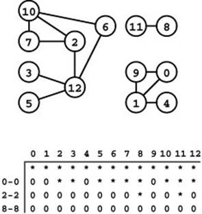
The table at the bottom shows vertex marks (contents of the ord vector) during a typical search of the graph at the top. Initially, the function GRAPHsearch in Program 18.2 unmarks all vertices by setting the marks all to -1 (indicated by an asterisk). Then it calls search for the dummy edge 0-0, which marks all of the vertices in the same connected component as 0 (second row) by setting them to a nonnegative values (indicated by 0s). In this example, it marks 0, 1, 4, and 9 with the values 0 through 3 in that order. Next, it scans from left to right to find the unmarked vertex 2 and calls search for the dummy edge 2-2 (third row), which marks the seven vertices in the same connected component as 2. Continuing the left-to-right scan, it calls search for 8-8 to mark 8 and 11 (bottom row). Finally, GRAPHsearch completes the search by discovering that 9 through 12 are all marked.
Program 18.3 Derived class for depth-first search
This code shows how we derive a spanning-forest DFS class from the base class defined in Program 18.2. The constructor builds a representation of the forest in st (parent links) along with ord (from the base class). Clients can use a DFS object to find any given vertex’s parent in the forest (ST), or any given vertex’s position in a preorder walk of the forest (overloaded [] operator). Properties of these forests and representations are the topic of Section 18.4.
template <class Graph>
class DFS : public SEARCH<Graph>
{ vector<int> st;
void searchC(Edge e)
{ int w = e.w;
ord[w] = cnt++; st[e.w] = e.v;
typename Graph::adjIterator A(G, w);
for (int t = A.beg(); !A.end(); t = A.nxt())
if (ord[t] == -1) searchC(Edge(w, t));
}
public:
DFS(const Graph &G) : SEARCH<Graph>(G),
st(G.V(), -1) { search(); }
int ST(int v) const { return st[v]; }
};
Property 18.2 A graph-search function checks each edge and marks each vertex in a graph if and only if the search function that it uses marks each vertex and checks each edge in the connected component that contains the start vertex.
Proof: By induction on the number of connected components. •
Graph-search functions provide a systematic way of processing each vertex and each edge in a graph. Generally, our implementations are designed to run in linear or near-linear time, by doing a fixed amount of processing per edge. We prove this fact now for DFS, noting that the same proof technique works for several other search strategies.
Property 18.3 DFS of a graph represented with an adjacency matrix requires time proportional to V2.
Proof: An argument similar to the proof of Property 18.1 shows that searchC not only marks all vertices connected to the start vertex but also calls itself exactly once for each such vertex (to mark that vertex). An argument similar to the proof of Property 18.2 shows that a call to search leads to exactly one call to searchC for each graph vertex. In searchC, the iterator checks every entry in the vertex’s row in the adjacency matrix. In other words, the search checks each entry in the adjacency matrix precisely once.•
Property 18.4 DFS of a graph represented with adjacency lists requires time proportional to V + E.
Proof: From the argument just outlined, it follows that we call the recursive function precisely V times (hence the V term), and we examine each entry on each adjacency list (hence the E term).•
The primary implication of Properties 18.3 and 18.4 is that they establish the running time of DFS to be linear in the size of the data structure used to represent the graph. In most situations, we are also justified in thinking of the running time of DFS as being linear in the size of the graph, as well: If we have a dense graph (with the number of edges proportional to V2) then either representation gives this result; if we have a sparse graph, then we assume use of an adjacency-lists representation. Indeed, we normally think of the running time of DFS as being linear in E. That statement is technically not true if we are using adjacency matrices for sparse graphs or for extremely sparse graphs with E << V and most vertices isolated, but we can usually avoid the former situation, and we can remove isolated vertices (see Exercise 17.34) in the latter situation.
As we shall see, these arguments all apply to any algorithm that has a few of the same essential features of DFS. If the algorithm marks each vertex and examines all the latter’s incident vertices (and does any other work that takes time per vertex bounded by a constant), then these properties apply. More generally, if the time per vertex is bounded by some function f (V, E), then the time for the search is guaranteed to be proportional to E + Vf (V, E). In Section 18.8, we see that DFS is one of a family of algorithms that has just these characteristics; in Chapters 19 through 22, we see that algorithms from this family serve as the basis for a substantial fraction of the code that we consider in this book.
Much of the graph-processing code that we examine is ADT-implementation code for some particular task, where we develop a class that does a basic search to compute structural information in other vertex-indexed vectors. We can derive the class from Program 18.2 or, in simple cases, just reimplement the search. Many of our graph-processing classes are of this nature because we typically can uncover a graph’s structure by searching it. We normally add code to the search function that is executed when each vertex is marked, instead of working with a more generic search (for example, one that calls a specified function each time a vertex is visited), solely to keep the code compact and self-contained. Providing a more general ADT mechanism for clients to process all the vertices with a client-supplied function is a worthwhile exercise (see Exercises 18.13 and18.14).
In Sections 18.5 and 18.6, we examine numerous graph-processing functions that are based on DFS. In Sections 18.7 and 18.8, we look at other implementations of search and at some graph-processing functions that are based on them. Although we do not build this layer of abstraction into our code, we take care to identify the basic graph-search strategy underlying each algorithm that we develop. For example, we use the term DFS class to refer to any implementation that is based on the recursive DFS scheme. The simple-path–search class Program 17.11 and the spanning-forest class Program 18.3 are examples of DFS classes.
Many graph-processing functions are based on the use of vertex-indexed vectors. We typically include such vectors as private data members in class implementations, to hold information about the structure of graphs (which is discovered during the search) that helps us solve the problem at hand. Examples of such vectors are the deg vector in Program 17.11 and the ord vector in Program 18.1. Some implementations that we will examine use multiple vectors to learn complicated structural properties.
Our convention in graph-search functions is to initialize all entries in vertex-indexed vectors to -1, and to set the entries corresponding to each vertex visited to nonnegative values in the search function. Any such vector can play the role of the ord vector (marking vertices as visited) in Programs 18.2 through 18.3. When a graph-search function is based on using or computing a vertex-indexed vector, we often just implement the search and use that vector to mark vertices, rather than deriving the class from SEARCH or maintaining the ord vector.
The specific outcome of a graph search depends not just on the nature of the search function but also on the graph representation and even the order in which search examines the vertices. For specificity in the examples and exercises in this book, we use the term standard adjacency-lists DFSto refer to the process of inserting a sequence of edges into a graph ADT implemented with an adjacency-lists representation (Program 17.9), then doing a DFS with, for example, Program 18.3. For the adjacency-matrix representation, the order of edge insertion does not affect search dynamics, but we use the parallel term standard adjacency-matrix DFS to refer to the process of inserting a sequence of edges into a graph ADT implemented with an adjacency-matrix representation (Program 17.7), then doing a DFS with, for example, Program 18.3.
Exercises
18.8 Show, in the style of Figure 18.5, a trace of the recursive function calls made for a standard adjacency-matrix DFS of the graph
3-7 1-4 7-8 0-5 5-2 3-8 2-9 0-6 4-9 2-6 6-4.
18.9 Show, in the style of Figure 18.7, a trace of the recursive function calls made for a standard adjacency-lists DFS of the graph
3-7 1-4 7-8 0-5 5-2 3-8 2-9 0-6 4-9 2-6 6-4.
18.10 Modify the adjacency-matrix graph ADT implementation in Program 17.7 to use a dummy vertex that is connected to all the other vertices. Then, provide a simplified DFS implementation that takes advantage of this change.
18.11 Do Exercise 18.10 for the adjacency-lists ADT implementation in Program 17.9.
• 18.12 There are 13! different permutations of the vertices in the graph depicted in Figure 18.8. How many of these permutations could specify the order in which vertices are visited by Program 18.2?
18.13 Implement a graph ADT client function that calls a client-supplied function for each vertex in the graph.
18.14 Implement a graph ADT client that calls a client-supplied function for each edge in the graph. Such a function might be a reasonable alternative to GRAPHedges (see Program 17.2).
Figure 18.9 DFS tree representations
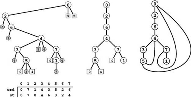
If we augment the DFS recursive-call tree to represent edges that are checked but not followed, we get a complete description of the DFS process (left). Each tree node has a child representing each of the nodes adjacent to it, in the order they were considered by the DFS, and a preorder traversal gives the same information as Figure 18.5: first we follow 0-0, then 0-2, then we skip 2-0, then we follow 2-6, then we skip 6-2, then we follow 6-4, then 4-3, and so forth. The ord vector specifies the order in which we visit tree vertices during this preorder walk, which is the same as the order in which we visit graph vertices in the DFS. The st vector is a parent-link representation of the DFS recursive-call tree (see Figure 18.6).
There are two links in the tree for every edge in the graph, one for each of the two times it encounters the edge. The first is to an unshaded node and either corresponds to making a recursive call (if it is to an internal node) or to skipping a recursive call because it goes to an ancestor for which a recursive call is in progress (if it is to an external node). The second is to a shaded external node and always corresponds to skipping a recursive call, either because it goes back to the parent (circles) or because it goes to a descendent of the parent for which a recursive call is in progress (squares). If we eliminate shaded nodes (center), then replace the external nodes with edges, we get another drawing of the graph (right).
All materials on the site are licensed Creative Commons Attribution-Sharealike 3.0 Unported CC BY-SA 3.0 & GNU Free Documentation License (GFDL)
If you are the copyright holder of any material contained on our site and intend to remove it, please contact our site administrator for approval.
© 2016-2025 All site design rights belong to S.Y.A.