Algorithms Third Edition in C++ Part 5. Graph Algorithms (2006)
CHAPTER SEVENTEEN
Graph Properties and Types
17.3 Adjacency-Matrix Representation
An adjacency-matrix representation of a graph is a V -by-V matrix of Boolean values, with the entry in row v and column w defined to be 1 if there is an edge connecting vertex v and vertex w in the graph, and to be 0 otherwise. Figure 17.8 depicts an example.
Program 17.7 is an implementation of the graph ADT interface that uses a direct representation of this matrix, built as a vector of vectors, as depicted in Figure 17.9. It is a two-dimensional existence table with the entry adj[v][w] set to true if there is an edge connecting v and w in the graph, and set to false otherwise. Note that maintaining this property in an undirected graph requires that each edge be represented by two entries: the edge v-w is represented by true values in both adj[v][w] and adj[w][v], as is the edge w-v.
The name DenseGRAPH in Program 17.7 emphasizes that the implementation is more suited for dense graphs than for sparse ones, and distinguishes it from other implementations. Clients may use typedef to make this type equivalent to GRAPH or use DenseGRAPH explicitly.
In the adjacency matrix that represents a graph G, row v is a vector that is an existence table whose ith entry is true if vertex i is adjacent to v (the edge v-i is in G). Thus, to provide clients with the capability to process the vertices adjacent to v, we need only provide code that scans through this vector to find true entries, as shown in Program 17.8. We need to be mindful that, with this implementation, processing all of the vertices adjacent to a given vertex requires (at least) time proportional to V, no matter how many such vertices exist.
As mentioned in Section 17.2, our interface requires that the number of vertices is known to the client when the graph is initialized. If desired, we could allow for inserting and deleting vertices (see Exercise 17.21). A key feature of the constructor in Program 17.7 is
Figure 17.8 Adjacency-matrix graph representation
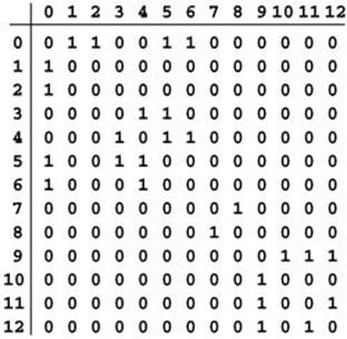
This Boolean matrix is another representation of the graph depicted in Figure 17.1. It has a 1 (true) in row v and column w if there is an edge connecting vertex v and vertex w and a 0 (false) in row v and column w if there is no such edge. The matrix is symmetric about the diagonal. For example, the sixth row (and the sixth column) says that vertex 6 is connected to vertices 0 and 4. For some applications, we will adopt the convention that each vertex is connected to itself, and assign 1s on the main diagonal. The large blocks of 0s in the upper right and lower left corners are artifacts of the way we assigned vertex numbers for this example, not characteristic of the graph (except that they do indicate the graph to be sparse).
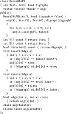
Program 17.7 Graph ADT implementation (adjacency matrix)
This class is a straightforward implementation of the interface in Program 17.1 that is based on representing the graph with a vector of boolean vectors (see Figure 17.9). Edges are inserted and removed in constant time. Duplicate edge insert requests are silently ignored, but clients can use edge to test whether an edge exists. Constructing the graph takes time proportional toV2.
Program 17.8 Iterator for adjacency-matrix representation
This implementation of the iterator for Program 17.7 uses an index i to scan past false entries in row v of the adjacency matrix (adj[v]). A call to beg() followed by a sequence of calls to nxt() (checking that end() is false before each call) gives a sequence of the vertices adjacent to v in G in order of their vertex index.
class DenseGRAPH::adjIterator
{ const DenseGRAPH &G;
int i, v;
public:
adjIterator(const DenseGRAPH &G, int v) :
G(G), v(v), i(-1) { }
int beg()
{ i = -1; return nxt(); }
int nxt()
{
for (i++; i < G.V(); i++)
if (G.adj[v][i] == true) return i;
return -1;
}
bool end()
{ return i >= G.V(); }
};
that it initializes the graph by setting the matrix entries all to false. We need to be mindful that this operation takes time proportional to V2, no matter how many edges are in the graph. Error checks for insufficient memory are not included in Program 17.7 for brevity—it is prudent programming practice to add them before using this code (see Exercise 17.24).
To add an edge, we set the indicated matrix entries to true (one for digraphs, two for undirected graphs). This representation does not allow parallel edges: If an edge is to be inserted for which the matrix entries are already 1, the code has no effect. In some ADT designs, it might be preferable to inform the client of the attempt to insert a parallel edge, perhaps using a return code from insert. This representation does allow self-loops: An edge v-v is represented by a nonzero entry in a[v][v].
Figure 17.9 Adjacency matrix data structure
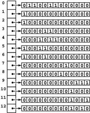
This figure depicts the C++ representation of the graph in Figure 17.1, as an vector of vectors.
To remove an edge, we set the indicated matrix entries to false. If a nonexistent edge (one for which the matrix entries are already false) is to be removed, the code has no effect. Again, in some ADT designs, we might wish to arrange to inform the client of such conditions.
If we are processing huge graphs or huge numbers of small graphs, or space is otherwise tight, there are several ways to save space. For example, adjacency matrices that represent undirected graphs are symmetric: a[v][w] is always equal to a[w][v]. Thus, we could save space by storing only one-half of this symmetric matrix (see Exercise 17.22). Another way to save a signigicant amount of space is to use a matrix of bits (assuming that vector<bool> does not do so). In this way, for instance, we could represent graphs of up to about 64,000 vertices in about 64 million 64-bit words (see Exercise 17.23). These implementations have the slight complication that we need to add an ADT operation to test for the existence of an edge (see Exercise 17.20). (We do not use such an operation in our implementations because we can test for the existence of an edge v-w by simply testing a[v][w].) Such space-saving techniques are effective, but come at the cost of extra overhead that may fall in the inner loop in time-critical applications.
Many applications involve associating other information with each edge—in such cases, we can generalize the adjacency matrix to hold any information whatever, not just bools. Whatever data type that we use for the matrix elements, we need to include an indication whether the indicated edge is present or absent. In Chapters 20 and 21, we explore such representations.
Use of adjacency matrices depends on associating vertex names with integers between 0 and V − 1. This assignment might be done in one of many ways—for example, we consider a program that does so in Section 17.6). Therefore, the specific matrix of 0-1 values that we represent with a vector of vectors in C++ is but one possible representation of any given graph as an adjacency matrix, because another program might assign different vertex names to the indices we use to specify rows and columns. Two matrices that appear to be markedly different could represent the same graph (see Exercise 17.17). This observation is a restatement of the graph isomorphism problem: Although we might like to determine whether or not two different matrices represent the same graph, no one has devised an algorithm that can always do so efficiently. This difficulty is fundamental. For example, our ability to find an efficient solution to various important graph-processing problems depends completely on the way in which the vertices are numbered (see, for example, Exercise 17.26).
Program 17.3, which we considered in Section 17.2, prints out a table with the vertices adjacent to each vertex. When used with the implementation in Program 17.7, it prints the vertices in order of their vertex index, as in Figure 17.7. Notice, though, that it is not part of the definition of adjIterator that it visits vertices in index order, so developing an ADT client that prints out the adjacency-matrix representation of a graph is not a trivial task (see Exercise 17.18). The output produced by these programs are themselves graph representations that clearly illustrate a basic performance tradeoff. To print out the matrix, we need room on the page for all V2 entries; to print out the lists, we need room for just V + E numbers. For sparse graphs, when V2 is huge compared to V + E, we prefer the lists; for dense graphs, when E and V2 are comparable, we prefer the matrix. As we shall soon see, we make the same basic tradeoff when we compare the adjacency-matrix representation with its primary alternative: an explicit representation of the lists.
The adjacency-matrix representation is not satisfactory for huge sparse graphs: We need at least V2 bits of storage and V2 steps just to construct the representation. In a dense graph, when the number of edges (the number of 1 bits in the matrix) is proportional to V2, this cost may be acceptable, because time proportional to V2 is required to process the edges no matter what representation we use. In a sparse graph, however, just initializing the matrix could be the dominant factor in the running time of an algorithm. Moreover, we may not even have enough space for the matrix. For example, we may be faced with graphs with millions of vertices and tens of millions of edges, but we may not want—or be able—to pay the price of reserving space for trillions of 0 entries in the adjacency matrix.
On the other hand, when we do need to process a huge dense graph, then the 0-entries that represent absent edges increase our space needs by only a constant factor and provide us with the ability to determine whether any particular edge is present in constant time. For example, disallowing parallel edges is automatic in an adjacency matrix but is costly in some other representations. If we do have space available to hold an adjacency matrix, and either V2 is so small as to represent a negligible amount of time or we will be running a complex algorithm that requires more than V2steps to complete, the adjacency-matrix representation may be the method of choice, no matter how dense the graph.
Exercises
• 17.17 Give the adjacency-matrix representations of the three graphs depicted in Figure 17.2.
• 17.18 Give an implementation of show for the representation-independent io package of Program 17.4 that prints out a two-dimensional matrix of 0s and 1s like the one illustrated in Figure 17.8. Note: You cannot depend upon the iterator producing vertices in order of their indices.
17.19 Given a graph, consider another graph that is identical to the first, except that the names of (integers corresponding to) two vertices are interchanged. How are the adjacency matrices of these two graphs related?
• 17.20 Add a function edge to the graph ADT that allows clients to test whether there is an edge connecting two given vertices, and provide an implementation for the adjacency-matrix representation.
• 17.21 Add functions to the graph ADT that allow clients to insert and delete vertices, and provide implementations for the adjacency-matrix representation.
• 17.22 Modify Program 17.7, augmented as described in Exercise 17.20, to cut its space requirements about in half by not including array entries a[v][w] for w greater than v.
17.23 Modify Program 17.7, augmented as described in Exercise 17.20, to ensure that, if your computer has B bits per word, a graph with V vertices is represented in about V2/B words (as opposed to V2). Do empirical tests to assess the effect of packing bits into words on the time required for the ADT operations.
17.24 Describe what happens if there is insufficient memory available to represent the matrix when the constructor in Program 17.7 is invoked, and suggest appropriate modifications to the code to handle this situation.
17.25 Develop a version of Program 17.7 that uses a single vector with V2 entries.
• 17.26 Suppose that all k vertices in a group have consecutive indices. How can you determine from the adjacency matrix whether or not that group of vertices constitutes a clique? Write a client ADT function that finds, in time proportional to V2, the largest group of vertices with consecutive indices that constitutes a clique.