Algorithms Third Edition in C++ Part 5. Graph Algorithms (2006)
CHAPTER TWENTY-ONE
Shortest Paths
21.1 Underlying Principles
Our shortest-paths algorithms are based on a simple operation known as relaxation. We start a shortest-paths algorithm knowing only the network’s edges and weights. As we proceed, we gather information about the shortest paths that connect various pairs of vertices. Our algorithms all update this information incrementally, making new inferences about shortest paths from the knowledge gained so far. At each step, we test whether we can find a path that is shorter than some known path. The term “relaxation” is commonly used to describe this step, which relaxes constraints on the shortest path. We can think of a rubber band stretched tight on a path connecting two vertices: A successful relaxation operation allows us to relax the tension on the rubber band along a shorter path.
Our algorithms are based on applying repeatedly one of two types of relaxation operations:
• Edge relaxation: Test whether traveling along a given edge gives a new shortest path to its destination vertex.
• Path relaxation: Test whether traveling through a given vertex gives a new shortest path connecting two other given vertices.
Edge relaxation is a special case of path relaxation; we consider the operations separately, however, because we use them separately (the former in single-source algorithms; the latter in all-pairs algorithms). In both cases, the prime requirement that we impose on the data structures that we use to represent the current state of our knowledge about a network’s shortest paths is that we can update them easily to reflect changes implied by a relaxation operation.
First, we consider edge relaxation, which is illustrated in Figure 21.5. All the single-source shortest-paths algorithms that we consider are based on this step: Does a given edge lead us to consider a shorter path to its destination from the source?
Figure 21.5 Edge relaxation
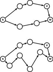
These diagrams illustrate the relaxation operation that underlies our single-source shortest-paths algorithms. We keep track of the shortest known path from the source s to each vertex and ask whether an edge v-w gives us a shorter path to w. In the top example, it does not; so we would ignore it. In the bottom example, it does; so we would update our data structures to indicate that the best known way to get to w from s is to go to v, then take v-w.
The data structures that we need to support this operation are straightforward. First, we have the basic requirement that we need to compute the shortest-paths lengths from the source to each of the other vertices. Our convention will be to store in a vertex-indexed vector wt the lengths of the shortest known paths from the source to each vertex. Second, to record the paths themselves as we move from vertex to vertex, our convention will be the same as the one that we used for other graph-search algorithms that we examined in Chapters 18 through 20: We use a vertex-indexed vector spt to record the last edge on a shortest path from the source to the indexed vertex. These edges constitute a tree.
With these data structures, implementing edge relaxation is a straightforward task. In our single-source shortest-paths code, we use the following code to relax along an edge e from v to w:
if (wt[w] > wt[v] + e->wt())
{ wt[w] = wt[v] + e->wt(); spt[w] = e; }
This code fragment is both simple and descriptive; we include it in this form in our implementations, rather than defining relaxation as a higher-level abstract operation.
Definition 21.2 Given a network and a designated vertex s, a shortest-paths tree (SPT) for s is a subnetwork containing s and all the vertices reachable from s that forms a directed tree rooted at s such that every tree path is a shortest path in the network.
There may be multiple paths of the same length connecting a given pair of nodes, so SPTs are not necessarily unique. In general, as illustrated in Figure 21.2, if we take shortest paths from a vertex s to every vertex reachable from s in a network and from the subnetwork induced by the edges in the paths, we may get a DAG. Different shortest paths connecting pairs of nodes may each appear as a subpath in some longer path containing both nodes. Because of such effects, we generally are content to compute any SPT for a given digraph and start vertex.
Our algorithms generally initialize the entries in the wt vector with a sentinel value. That value needs to be sufficiently small that the addition in the relaxation test does not cause overflow and sufficiently large that no simple path has a larger weight. For example, if edge weights are between 0 and 1, we can use the value V. Note that we have to take extra care to check our assumptions when using sentinels in networks that could have negative weights. For example, if both vertices have the sentinel value, the relaxation code just given takes no action if e.wt is nonnegative (which is probably what we intend in most implementations), but it will change wt[w] and spt[w] if the weight is negative.
Our code always uses the destination vertex as the index to save the SPT edges (spt[w]->w() == w). For economy and consistency with Chapters 17 through 19, we use the notation st[w] to refer to the vertex spt[w]->v() (in the text and particularly in the figures) to emphasize that the spt vector is actually a parent-link representation of
Figure 21.6 Shortest paths trees
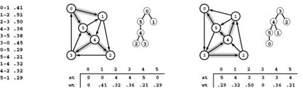
The shortest paths from 0 to the other nodes in this network are 0-1, 0-5-4-2, 0-5-4-3, 0-5-4, and 0-5, respectively. These paths define a spanning tree, which is depicted in three representations (gray edges in the network drawing, oriented tree, and parent links with weights) in the center. Links in the parent-link representation (the one that we typically compute) run in the opposite direction than links in the digraph, so we sometimes work with the reverse digraph. The spanning tree defined by shortest paths from 3 to each of the other nodes in the reverse is depicted on the right. The parent-link representation of this tree gives the shortest paths from each of the other nodes to 2 in the original graph. For example, we can find the shortest path 0-5-4-3 from 0 to 3 by following the links st[0] = 5, st[5] = 4, and st[4] = 3.
the shortest-paths tree, as illustrated in Figure 21.6. We can compute the shortest path from s to t by traveling up the tree from t to s;when we do so, we are traversing edges in the direction opposite from their direction in the network and are visiting the vertices on the path in reverse order (t, st[t], st[st[t]], and so forth).
One way to get the edges on the path in order from source to sink from an SPT is to use a stack. For example, the following code prints a path from the source to a given vertex w:
stack <EDGE *> P; EDGE *e = spt[w];
while (e) { P.push(e); e = spt[e->v()]); }
if (P.empty()) cout << P.top()->v();
while (!P.empty())
{ cout << ’-’ << P.top()->w(); P.pop(); }
In a class implementation, we could use code similar to this to provide clients with a vector that contains the edges of the path.
If we simply want to print or otherwise process the edges on the path, going all the way through the path in reverse order to get to the first edge in this way may be undesirable. One approach to get around this difficulty is to work with the reverse network, as illustrated in Figure 21.6. We use reverse order and edge relaxation in single-source problems because the SPT gives a compact representation of the shortest paths from the source to all the other vertices, in a vector with just V entries.
Next, we consider path relaxation, which is the basis of some of our all-pairs algorithms: Does going through a given vertex lead us to a shorter path that connects two other given vertices? For example, suppose that, for three vertices s, x, and t, we wish to know whether it is better to go froms to x and then from x to t or to go from s to t without going through x. For straight-line connections in a Euclidean space, the triangle inequality tells us that the route through x cannot be shorter than the direct route from s to t, but for paths in a network, it could be (see Figure 21.7). To determine which, we need to know the lengths of paths from s to x, x to t, and of those from s to t (that do not include x). Then, we simply test whether or not the sum of the first two is less than the third; if it is, we update our records accordingly.
Path relaxation is appropriate for all-pairs solutions where we maintain the lengths of the shortest paths that we have encountered between all pairs of vertices. Specifically, in all-pairs–shortest-paths code of this kind, we maintain a vector of vectors d such that d[s][t] is the shortest-path length from s to t, and we also maintain a vector of vectors p such that p[s][t] is the next vertex on a shortest path from s to t. We refer to the former as the distances matrix and the latter as the paths matrix. Figure 21.8 shows the two matrices for our example network. The distances matrix is a prime objective of the computation, and we use the paths matrix because it is clearly more compact than, but carries the same information as, the full list of paths that is illustrated in Figure 21.3.
Figure 21.7 Path relaxation

These diagrams illustrate the relaxation operation that underlies our all-pairs shortest-paths algorithms. We keep track of the best known path between all pairs of vertices and ask whether a vertex i is evidence that the shortest known path from s to t could be improved. In the top example, it is not; in the bottom example, it is. Whenever we encounter a vertex i such that the length of the shortest known path from s to i plus the length of the shortest known path from i to t is smaller than the length of the shortest known path from s to t, then we update our data structures to indicate that we now know a shorter path from s to t (head towards i first).
In terms of these data structures, path relaxation amounts to the following code:
if (d[s][t] > d[s][x] + d[x][t])
{ d[s][t] = d[s][x] + d[x][t]; p[s][t] = p[s][x]; }
Like edge relaxation, this code reads as a restatement of the informal description that we have given, so we use it directly in our implementations. More formally, path relaxation reflects the following.
Property 21.1 If a vertex x is on a shortest path from s to t, then that path consists of a shortest path from s to x followed by a shortest path from x to t.
Proof: By contradiction. We could use any shorter path from s to x or from x to t to build a shorter path from s to t.
We encountered the path-relaxation operation when we discussed transitive-closure algorithms, in Section 19.3. If the edge and path weights are either 1 or infinite (that is, a path’s weight is 1 only if all that path’s edges have weight 1), then path relaxation is the operation that we used in Warshall’s algorithm (if we have a path from s to x and a path from x to t, then we have a path from s to t). If we define a path’s weight to be the number of edges on that path, then
Figure 21.8 All shortest paths
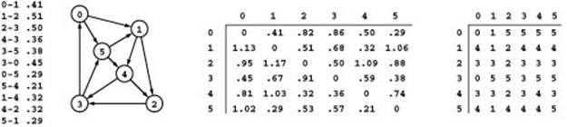
The two matrices on the right are compact representations of all the shortest paths in the sample network on the left, containing the same information in the exhaustive list in Figure 21.3. The distances matrix on the left contains the shortest-path length: The entry in row s and column t is the length of the shortest path from s to t. The paths matrix on the right contains the information needed to execute the path: The entry in row s and column t is the next vertex on the path from s to t.
Warshall’s algorithm generalizes to Floyd’s algorithm for finding all shortest paths in unweighted digraphs; it further generalizes to apply to networks, as we see in Section 21.3.
From a mathematician’s perspective, it is important to note that these algorithms all can be cast in a general algebraic setting that unifies and helps us to understand them. From a programmer’s perspective, it is important to note that we can implement each of these algorithms using an abstract + operator (to compute path weights from edge weights) and an abstract < operator (to compute the minimum value in a set of path weights), both solely in the context of the relaxation operation (see Exercises 19.55 and 19.56).
Property 21.1 implies that a shortest path from s to t contains shortest paths from s to every other vertex along the path to t. Most shortest-paths algorithms also compute shortest paths from s to every vertex that is closer to s than to t (whether or not the vertex is on the path from s to t), although that is not a requirement (see Exercise 21.18). Solving the source–sink shortest-paths problem with such an algorithm when t is the vertex that is farthest from s is equivalent to solving the single-source shortest-paths problem for s. Conversely, we could use a solution to the single-source shortest-paths problem from s as a method for finding the vertex that is farthest from s.
The paths matrix that we use in our implementations for the all-pairs problem is also a representation of the shortest-paths trees for each of the vertices. We defined p[s][t] to be the vertex that follows s on a shortest path from s to t. It is thus the same as the vertex that precedes s on the shortest path from t to s in the reverse network. In other words, column t in the paths matrix of a network is a vertex-indexed vector that represents the SPT for vertex t in its reverse. Conversely, we can build the paths matrix for a network by
Figure 21.9 All shortest paths in a network
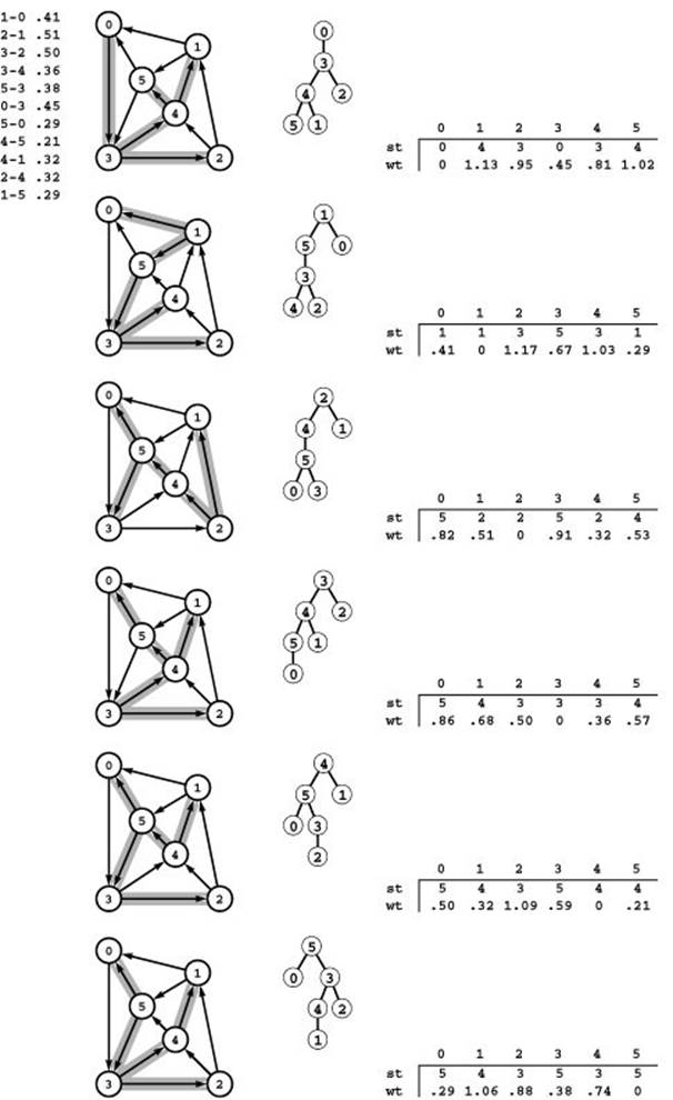
These diagrams depict the SPTs for each vertex in the reverse of the network in Figure 21.8 (0 to 5, top to bottom), as network subtrees (left), oriented trees (center), and parent-link representation including a vertex-indexed array for path length (right). Putting the arrays together to form path and distance matrices (where each array becomes a column) gives the solution to the all-pairs shortest-paths problem illustrated in Figure 21.8.
filling each column with the vertex-indexed vector representation of the SPT for the appropriate vertex in the reverse. This correspondence is illustrated in Figure 21.9.
In summary, relaxation gives us the basic abstract operations that we need to build our shortest paths algorithms. The primary complication is the choice of whether to provide the first or final edge on the shortest path. For example, single-source algorithms are more naturally expressed by providing the final edge on the path so that we need only a single vertex-indexed vector to reconstruct the path, since all paths lead back to the source. This choice does not present a fundamental difficulty because we can either use the reverse graph as warranted or provide member functions that hide this difference from clients. For example, we could specify a member function in the interface that returns the edges on the shortest path in a vector (see Exercises 21.15 and 21.16).
Accordingly, for simplicity, all of our implementations in this chapter include a member function dist that returns a shortest-path length and either a member function path that returns the first edge on a shortest path or a member function pathR that returns the final edge on a shortest path. For example, our single-source implementations that use edge relaxation typically implement these functions as follows:
Edge *pathR(int w) const { return spt[w]; }
double dist(int v) { return wt[v]; }
Similarly, our all-paths implementations that use path relaxation typically implement these functions as follows:
Edge *path(int s, int t) { return p[s][t]; }
double dist(int s, int t) { return d[s][t]; }
In some situations, it might be worthwhile to build interfaces that standardize on one or the other or both of these options; we choose the most natural one for the algorithm at hand.
Exercises
• 21.12 Draw the SPT from 0 for the network defined in Exercise 21.1 and for its reverse. Give the parent-link representation of both trees.
21.13 Consider the edges in the network defined in Exercise 21.1 to be undirected edges such that each edge corresponds to equal-weight edges in both directions in the network. Answer Exercise 21.12 for this corresponding network.
• 21.14 Change the direction of edge 0-2 in Figure 21.2. Draw two different SPTs that are rooted at 2 for this modified network.
21.15 Write a function that uses the pathR member function from a single-source implementation to put pointers to the edges on the path from the source v to a given vertex w in an STL vector.
21.16 Write a function that uses the path member function from an all-paths implementation to put pointers to the edges on the path from a given vertex v to another given vertex w in an STL vector.
21.17 Write a program that uses your function from Exercise 21.16 to print out all of the paths, in the style of Figure 21.3.
21.18 Give an example that shows how we could know that a path from s to t is shortest without knowing the length of a shorter path from s to x for some x.