Algorithms Third Edition in C++ Part 5. Graph Algorithms (2006)

CHAPTER TWENTY-ONE
Shortest Paths

21.2 Dijkstra’s Algorithm

In Section 20.3, we discussed Prim’s algorithm for finding the minimum spanning tree (MST) of a weighted undirected graph: We build it one edge at a time, always taking next the shortest edge that connects a vertex on the MST to a vertex not yet on the MST. We can use a nearly identical scheme to compute an SPT. We begin by putting the source on the SPT; then, we build the SPT one edge at a time, always taking next the edge that gives a shortest path from the source to a vertex not on the SPT. In other words, we add vertices to the SPT in order of their distance (through the SPT) to the start vertex. This method is known as Dijkstra’s algorithm.

As usual, we need to make a distinction between the algorithm at the level of abstraction in this informal description and various concrete implementations (such as Program 21.1) that differ primarily in graph representation and priority-queue implementations, even though such a distinction is not always made in the literature. We shall consider other implementations and discuss their relationships with Program 21.1 after establishing that Dijkstra’s algorithm correctly performs the single-source shortest-paths computation.

Property 21.2 Dijkstra’s algorithm solves the single-source shortest-paths problem in networks that have nonnegative weights.

Proof: Given a source vertex s, we have to establish that the tree path from the root s to each vertex x in the tree computed by Dijkstra’s algorithm corresponds to a shortest path in the graph from s to x. This fact follows by induction. Assuming that the subtree so far computed has the property, we need only to prove that adding a new vertex x adds a shortest path to that vertex. But all other paths to x must begin with a tree path followed by an edge to a vertex not on the tree. By construction, all such paths are longer than the one from s to x that is under consideration.

The same argument shows that Dijkstra’s algorithm solves the source–sink shortest-paths problem, if we start at the source and stop when the sink comes off the priority queue.

The proof breaks down if the edge weights could be negative, because it assumes that a path’s length does not decrease when we add more edges to the path. In a network with negative edge weights, this assumption is not valid because any edge that we encounter might lead to some tree vertex and might have a sufficiently large negative weight to give a path to that vertex shorter than the tree path. We consider this defect in Section 21.7 (see Figure 21.28).

Figure 21.10 shows the evolution of an SPT for a sample graph when computed with Dijkstra’s algorithm; Figure 21.11 shows an oriented drawing of a larger SPT tree. Although Dijkstra’s algorithm differs from Prim’s MST algorithm in only the choice of priority, SPT trees are different in character from MSTs. They are rooted at the start vertex and all edges are directed away from the root, whereas MSTs are unrooted and undirected. We sometimes represent MSTs as directed, rooted trees when we use Prim’s algorithm, but such structures are still different in character from SPTs (compare the oriented drawing in Figure 20.9 with the drawing in Figure 21.11). Indeed, the nature of the SPT somewhat depends on the choice of start vertex as well, as depicted in Figure 21.12.

Dijkstra’s original implementation, which is suitable for dense graphs, is precisely like Prim’s MST algorithm. Specifically, we simply change the assignment of the priority P in Program 20.6 from

P = e->wt()

(the edge weight) to

P = wt[v] + e->wt()

(the distance from the source to the edge’s destination). This change gives the classical implementation of Dijkstra’s algorithm: We grow

Figure 21.10 Dijkstra’s algorithm

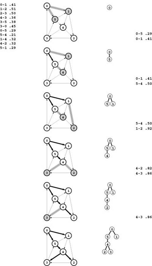
This sequence depicts the construction of a shortest-paths spanning tree rooted at vertex 0 by Dijkstra’s algorithm for a sample network. Thick black edges in the network diagrams are tree edges, and thick gray edges are fringe edges. Oriented drawings of the tree as it grows are shown in the center, and a list of fringe edges is given on the right.

The first step is to add 0 to the tree and the edges leaving it, 0-1 and 0-5, to the fringe (top). Second, we move the shortest of those edges, 0-5, from the fringe to the tree and check the edges leaving it: The edge 5-4 is added to the fringe and the edge 5-1 is discarded because it is not part of a shorter path from 0 to 1 than the known path 0-1 (second from top). The priority of 5-4 on the fringe is the length of the path from 0 that it represents, 0-5-4. Third, we move 0-1 from the fringe to the tree, add 1-2 to the fringe, and discard 1-4 (third from top). Fourth, we move 5-4 from the fringe to the tree, add 4-3 to the fringe, and replace 1-2 with 4-2 because 0-5-4-2 is a shorter path than 0-1-2 (fourth from top). We keep at most one edge to any vertex on the fringe, choosing the one on the shortest path from 0. We complete the computation by moving 4-2 and then 4-3 from the fringe to the tree (bottom).

Figure 21.11 Shortest-paths spanning tree

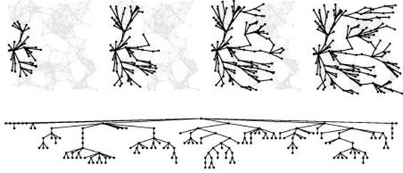
This figure illustrates the progress of Dijkstra’s algorithm in solving the single-source shortest-paths problem in a random Euclidean near-neighbor digraph (with directed edges in both directions corresponding to each line drawn), in the same style as Figures 18.13, 18.24, and 20.9. The search tree is similar in character to BFS because vertices tend to be connected to one another by short paths, but it is slightly deeper and less broad because distances lead to slightly longer paths than path lengths.

an SPT one edge at a time, each time updating the distance to the tree of all vertices adjacent to its destination while at the same time checking all the nontree vertices to find an edge to move to the tree whose destination vertex is a nontree vertex of minimal distance from the source.

Property 21.3 With Dijkstra’s algorithm, we can find any SPT in a dense network in linear time.

Proof: As for Prim’s MST algorithm, it is immediately clear, from inspection of the code of Program 20.6, that the running time is proportional to V², which is linear for dense graphs.

For sparse graphs, we can do better, by viewing Dijkstra’s algorithm as a generalized graph-searching method that differs from depth-first search (DFS), from breadth-first search (BFS), and from Prim’s MST algorithm in only the rule used to add edges to the tree. As in Chapter 20, we keep edges that connect tree vertices to non-tree vertices on a generalized queue called the fringe, use a priority queue to implement the generalized queue, and provide for updating priorities so as to encompass DFS, BFS, and Prim’s algorithm in a single implementation (see Section 20.3). This priority-first search (PFS) scheme also encompasses Dijkstra’s algorithm. That is, changing the assignment of P in Program 20.7 to

P = wt[v] + e->wt()

(the distance from the source to the edge’s destination) gives an implementation of Dijkstra’s algorithm that is suitable for sparse graphs.

Program 21.1 is an alternative PFS implementation for sparse graphs that is slightly simpler than Program 20.7 and that directly matches the informal description of Dijkstra’s algorithm given at the beginning of this section. It differs from Program 20.7 in that it initializes the priority queue with all the vertices in the network and maintains the queue with the aid of a sentinel value for those vertices that are neither on the tree nor on the fringe (unseen vertices with sentinel values); in contrast, Program 20.7 keeps on the priority queue only those vertices that are reachable by a single edge from the tree. Keeping all the vertices on the queue simplifies the code but can incur a small performance penalty for some graphs (see Exercise 21.31).

The general results that we considered concerning the performance of priority-first search (PFS) in Chapter 20 give us specific information about the performance of these implementations of Dijkstra’s algorithm for sparse graphs (Program 21.1 and Program 20.7, suitably modified). For reference, we restate those results in the present context. Since the proofs do not depend on the priority function, they apply without modification. They are worst-case results that apply to both programs, although Program 20.7 may be more efficient for many classes of graphs because it maintains a smaller fringe.

Property 21.4 For all networks and all priority functions, we can compute a spanning tree with PFS in time proportional to the time required for V insert , V delete the minimum , and E decrease key operations in a priority queue of size at most V.

Proof: This fact is immediate from the priority-queue–based implementations in Program 20.7 or Program 21.1. It represents a conservative upper bound because the size of the priority queue is often much smaller than V, particularly for Program 20.7.

Property 21.5 With a PFS implementation of Dijkstra’s algorithm that uses a heap for the priority-queue implementation, we can compute any SPT in time proportional to E lg V.

Program 21.1 Dijkstra’s algorithm (priority-first search)

This class implements a single-source shortest-paths ADT with linear-time preprocessing, private data that takes space proportional to V, and constant-time member functions that give the length of the shortest path and the final vertex on the path from the source to any given vertex. The constructor is an implementation of Dijkstra’s algorithm that uses a priority queue of vertices (in order of their distance from the source) to compute an SPT. The priority-queue interface is the same one used in Program 20.7 and implemented in Program 20.10.

The constructor is also a generalized graph search that implements other PFS algorithms with other assignments to the priority P (see text). The statement to reassign the weight of tree vertices to 0 is needed for a general PFS implementation but not for Dijkstra’s algorithm, since the priorities of the vertices added to the SPT are nondecreasing.

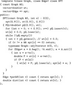
Figure 21.12 SPT examples

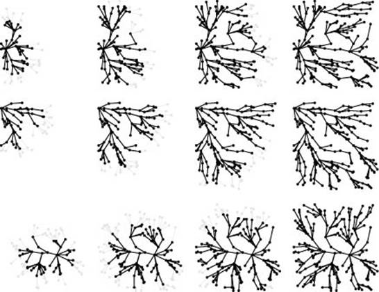
These three examples show growing SPTs for three different source locations: left edge (top), upper left corner (center), and center (bottom).

Proof: This result is a direct consequence of Property 21.4.

Property 21.6 Given a graph with V vertices and E edges, let d denote the density E/V. If d < 2, then the running time of Dijkstra’s algorithm is proportional to V lg V. Otherwise, we can improve the worst-case running time by a factor of lg(E/V), to O (E lg_d V ) (which is linear if E is at least V^1+ε)by using a E/V -ary heap for the priority queue.

Proof: This result directly mirrors Property 20.12 and the multiway-heap priority-queue implementation discussed directly thereafter.

Table 21.1 Priority-first search algorithms

These four classical graph-processing algorithms all can be implemented with PFS, a generalized priority-queue–based graph search that builds graph spanning trees one edge at a time. Details of search dynamics depend upon graph representation, priority-queue implementation, and PFS implementation; but the search trees generally characterize the various algorithms, as illustrated in the figures referenced in the fourth column.

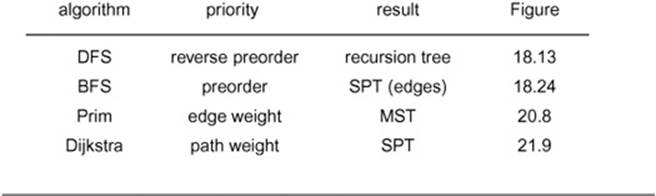
Table 21.1 summarizes pertinent information about the four major PFS algorithms that we have considered. They differ in only the priority function used, but this difference leads to spanning trees that are entirely different from one another in character (as required). For the example in the figures referred to in the table (and for many other graphs), the DFS tree is tall and thin, the BFS tree is short and fat, the SPT is like the BFS tree but neither quite as short nor quite as fat, and the MST is neither short and fat nor tall and thin.

We have also considered four different implementations of PFS. The first is the classical dense-graph implementation that encompasses Dijkstra’s algorithm and Prim’s MST algorithm (Program 20.6); the other three are sparse-graph implementations that differ in priority-queue contents:

• Fringe edges (Program 18.10)

• Fringe vertices (Program 20.7)

• All vertices (Program 21.1)

Of these, the first is primarily of pedagogical value, the second is the most refined of the three, and the third is perhaps the simplest. This framework already describes 16 different implementations of classical graph-search algorithms—when we factor in different priority-queue implementations, the possibilities multiply further. This proliferation

Table 21.2 Cost of implementations of Dijkstra’s algorithm

This table summarizes the cost (worst-case running time) of various implementations of Dijkstra’s algorithm. With appropriate priority-queue implementations, the algorithm runs in linear time (time proportional to V² for dense networks, E for sparse networks), except for networks that are extremely sparse.

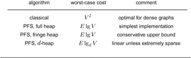
of networks, algorithms, and implementations underscores the utility of the general statements about performance in Properties 21.4 through 21.6, which are also summarized in Table 21.2.

As is true of MST algorithms, actual running times of shortest-paths algorithms are likely to be lower than these worst-case time bounds suggest, primarily because most edges do not necessitate decrease key operations. In practice, except for the sparsest of graphs, we regard the running time as being linear.

The name Dijkstra’s algorithm is commonly used to refer both to the abstract method of building an SPT by adding vertices in order of their distance from the source and to its implementation as the V² algorithm for the adjacency-matrix representation, because Dijkstra presented both in his 1959 paper (and also showed that the same approach could compute the MST). Performance improvements for sparse graphs are dependent on later improvements in ADT technology and priority-queue implementations that are not specific to the shortest-paths problem. Improved performance of Dijkstra’s algorithm is one of the most important applications of that technology (see reference section). As with MSTs, we use terminology such as the “PFS implementation of Dijkstra’s algorithm using d -heaps” to identify specific combinations.

We saw in Section 18.8 that, in unweighted undirected graphs, using preorder numbering for priorities causes the priority queue to operate as a FIFO queue and leads to a BFS. Dijkstra’s algorithm gives us another realization of BFS: When all edge weights are 1, it visits vertices in order of the number of edges on the shortest path to the start vertex. The priority queue does not operate precisely as a FIFO queue would in this case, because items with equal priority do not necessarily come out in the order in which they went in.

Each of these implementations puts the edges of an SPT from vertex 0 in the vertex-indexed vector spt, with the shortest-path length to each vertex in the SPT in the vertex-indexed vector wt and provides member functions that gives clients access to this data. As usual, we can build various graph-processing functions and classes around this basic data (see Exercises 21.21 through 21.28).

Exercises

• 21.19 Show, in the style of Figure 21.10, the result of using Dijkstra’s algorithm to compute the SPT of the network defined in Exercise 21.1 with start vertex 0.

• 21.20 How would you find a second shortest path from s to t in a network?

21.21 Write a client function that uses an SPT object to find the most distant vertex from a given vertex s (the vertex whose shortest path from s is the longest).

21.22 Write a client function that uses an SPT object to compute the average of the lengths of the shortest paths from a given vertex to each of the vertices reachable from it.

21.23 Develop a class based on Program 21.1 with a path member function that returns an STL vector containing pointers to the edges on the shortest path connecting s and t in order from s to t on an STL vector.

• 21.24 Write a client function that uses your class from Exercise 21.23 to print the shortest paths from a given vertex to each of the other vertices in a given network.

21.25 Write a client function that uses an SPT object to find all vertices within a given distance d of a given vertex in a given network. The running time of your function should be proportional to the size of the subgraph induced by those vertices and the vertices incident on them.

21.26 Develop an algorithm for finding an edge whose removal causes maximal increase in the shortest-path length from one given vertex to another given vertex in a given network.

• 21.27 Implement a class that uses SPT objects to perform a sensitivity analysis on the network’s edges with respect to a given pair of vertices s and t: Compute a V-by-V matrix such that, for every u and v, the entry in row u and column v is 1 if u-v is an edge in the network whose weight can be increased without the shortest-path length from s to t being increased and is 0 otherwise.

• 21.28 Implement a class that uses SPT objects to find a shortest path connecting one given set of vertices with another given set of vertices in a given network.

21.29 Use your solution from Exercise 21.28 to implement a client function that finds a shortest path from the left edge to the right edge in a random grid network (see Exercise 20.17).

21.30 Show that an MST of an undirected graph is equivalent to a bottleneck SPT of the graph: For every pair of vertices v and w, it gives the path connecting them whose longest edge is as short as possible.

21.31 Run empirical studies to compare the performance of the two versions of Dijkstra’s algorithm for the sparse graphs that are described in this section (Program 21.1 and Program 20.7, with suitable priority definition), for various networks (see Exercises 21.4–8). Use a standard-heap priority-queue implementation.

21.32 Run empirical studies to learn the best value of d when using a d-heap priority-queue implementation (see Program 20.10) for each of the three PFS implementations that we have discussed (Program 18.10, Program 20.7 and Program 21.1), for various networks (see Exercises 21.4–8).

• 21.33 Run empirical studies to determine the effect of using an index-heap-tournament priority-queue implementation (see Exercise 9.53) in Program 21.1, for various networks (see Exercises 21.4–8).

• 21.34 Run empirical studies to analyze height and average path length in SPTs, for various networks (see Exercises 21.4–8).

21.35 Develop a class for the source–sink shortest-paths problem that is based on code like Program 21.1 but that initializes the priority queue with both the source and the sink. Doing so leads to the growth of an SPT from each vertex; your main task is to decide precisely what to do when the two SPTs collide.

• 21.36 Describe a family of graphs with V vertices and E edges for which the worst-case running time of Dijkstra’s algorithm is achieved.

• 21.37 Develop a reasonable generator for random graphs with V vertices and E edges for which the running time of the heap-based PFS implementation of Dijkstra’s algorithm is superlinear.

• 21.38 Write a client program that does dynamic graphical animations of Dijkstra’s algorithm. Your program should produce images like Figure 21.11 (see Exercises 17.56 through 17.60). Test your program on random Euclidean networks (see Exercise 21.9).