Algorithms Third Edition in C++ Part 5. Graph Algorithms (2006)
CHAPTER TWENTY-TWO
Network Flow
22.3 Preflow-Push Maxflow Algorithms
In this section, we consider another approach to solving the maxflow problem. Using a generic method known as the preflow-push method, we incrementally move flow along the outgoing edges of vertices that have more inflow than outflow. The preflow-push approach was developed by A. Goldberg and R. E. Tarjan in 1986 on the basis of various earlier algorithms. It is widely used because of its simplicity, flexibility, and efficiency.
As defined in Section 22.1, a flow must satisfy the equilibrium conditions that the outflow from the source is equal to the inflow to the sink and that inflow is equal to the outflow at each of the internal nodes. We refer to such a flow as a feasible flow. An augmenting-path algorithm always maintains a feasible flow: It increases the flow along augmenting paths until a maxflow is achieved. By contrast, the preflow-push algorithms that we consider in this section maintain maxflows that are not feasible because some vertices have more inflow than outflow: They push flow through such vertices until a feasible flow is achieved (no such vertices remain).
Definition 22.5 In a flow network, a preflow is a set of positive edge flows satisfying the conditions that the flow on each edge is no greater than that edge’s capacity and that inflow is no smaller than outflow
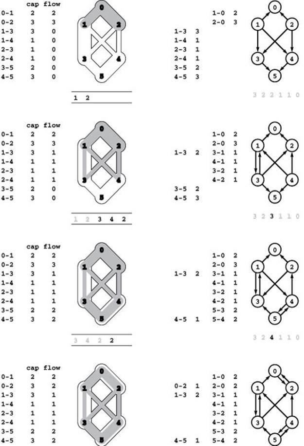
Figure 22.25 Preflow-push example
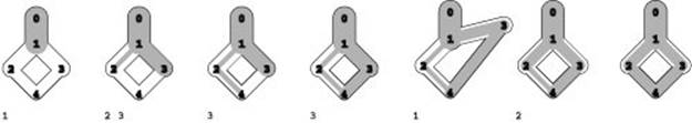
In the preflow-push algorithm, we maintain a list of the active nodes that have more incoming than outgoing flow (shown below each network). One version of the algorithm is a loop that chooses an active node from the list and pushes flow along outgoing edges until it is no longer active, perhaps creating other active nodes in the process. In this example, we push flow along 0-1, which makes 1 active. Next, we push flow along 1-2 and 1-3, which makes 1 inactive but 2 and 3 both active. Then, we push flow along 2-4, which makes 2 inactive. But 3-4 does not have sufficient capacity for us to push flow along it to make 3 inactive, so we also push flow back along 3-1 to do so, which makes 1 active. Then we can push the flow along 1-2 and then 2-4, which makes all nodes inactive and leaves a maxflow.
for every internal vertex. An active vertex is an internal vertex whose inflow is larger than its outflow (by convention, the source and sink are never active).
We refer to the difference between an active vertex’s inflow and outflow as that vertex’s excess. To change the set of active vertices, we choose one and push its excess along an outgoing edge, or, if there is insufficient capacity to do so, push the excess back along an incoming edge. If the push equalizes the vertex’s inflow and outflow, the vertex becomes inactive; the flow pushed to another vertex may activate that vertex. The preflow-push method provides a systematic way to push excess out of active vertices repeatedly so that the process terminates in a maxflow, with no active vertices. We keep active vertices on a generalized queue. As for the augmenting-path method, this decision gives a generic algorithm that encompasses a whole family of more specific algorithms.
Figure 22.25 is a small example that illustrates the basic operations used in preflow-push algorithms, in terms of the metaphor that we have been using, where we imagine that flow can go only down the page. Either we push excess flow out of an active vertex down an outgoing edge or we imagine that the vertex temporarily moves up so we can push excess flow back down an incoming edge.
Figure 22.26 is an example that illustrates why the preflow-push approach might be preferred to the augmenting-paths approach. In this network, any augmenting-path method successively puts a tiny amount of flow through a long path over and over again, slowly filling up the edges on the path until finally the maxflow is reached. By contrast, the preflow-push method fills up the edges on the long path as it traverses that path for the first time, then distributes that flow directly to the sink without traversing the long path again.
As we did in augmenting-path algorithms, we use the residual network (see Definition 22.4) to keep track of the edges that we might push flow through. Every edge in the residual network represents a potential place to push flow. If a residual-network edge is in the same direction as the corresponding edge in the flow network, we increase the flow; if it is in the opposite direction, we decrease the flow. If the increase fills the edge or the decrease empties the edge, the corresponding edge disappears from the residual network. For preflow-push algorithms, we use an additional mechanism to help decide which of the edges in the residual network can help us to eliminate active vertices.
Definition 22.6 A height function for a given flow in a flow network is a set of nonnegative vertex weights h(0)…h(V− 1)such that h (t)= 0 for the sink t and h(u)≤h(v)+1for every edge u-v in the residual network for the flow. An eligible edge is an edge u-v in the residual network with h(u)=h(v)+1.
Figure 22.26 Bad case for the Ford–Fulkerson algorithm
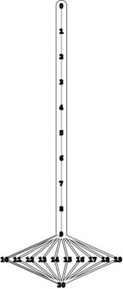
This network represents a family of networks with V vertices for which any augmenting-path algorithm requires V/ 2 paths of length V/2 (since every augmenting path has to include the long vertical path), for a total running time proportional to V2. Preflow-push algorithms find maxflows in such networks in linear time.
A trivial height function, for which there are no eligible edges, is h(0)=h(1) =…=h(V − 1) = 0. If we set h(s) = 1, then any edge that emanates from the source and has flow corresponds to an eligible edge in the residual network.
We define a more interesting height function by assigning to each vertex the latter’s shortest-path distance to the sink (its distance to the root in any BFS tree for the reverse of the network rooted at t, as illustrated in Program 22.27). This height function is valid because h(t) = 0, and, for any pair of vertices u and v connected by an edge u-v, any shortest path to t starting with u-v is of length h (v) + 1; so the shortest-path length from u to t, or h (u), must be less than or equal to that value. This function plays a special role because it puts each vertex at the maximum possible height. Working backward, we see that t has to be at height 0; the only vertices that could be at height 1 are those with an edge directed to t in the residual network; the only vertices that could be at height 2 are those that have edges directed to vertices that could be at height 1, and so forth.
Property 22.9 For any flow and associated height function, a vertex’s height is no larger than the length of the shortest path from that vertex to the sink in the residual network.
Proof: For any given vertex u, let d be the shortest-path length from u to t, and let u =u1, u2,…, ud =t be a shortest path. Then
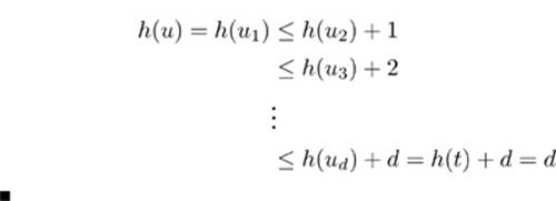
Figure 22.27 Initial height function
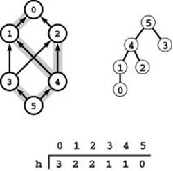
The tree at the right is a BFS tree rooted at 5 for the reverse of our sample network (left). The vertex-indexed array h gives the distance from each vertex to the root and is a valid height function: For every edge u-v in the network, h[u] is less than or equal to h[v]+1.
The intuition behind height functions is the following: When an active node’s height is less than the height of the source, it is possible that there is some way to push flow from that node down to the sink; when an active node’s height exceeds the height of the source, we know that that node’s excess needs to be pushed back to the source. To establish this latter fact, we reorient our view of Property 22.9, where we thought about the length of the shortest path to the sink as an upper bound on the height; instead, we think of the height as a lower bound on the shortest-path length:
Corollary If a vertex’s height is greater than V, then there is no path from that vertex to the sink in the residual network.
Proof: If there is a path from the vertex to the sink, the implication of Property 22.9 would be that the path’s length is greater than V, but that cannot be true because the network has only V vertices.
Now that we understand these basic mechanisms, the generic preflow-push algorithm is simple to describe. We start with any height function and assign zero flow to all edges except those connected to the source, which we fill to capacity. Then, we repeat the following step until no active vertices remain:
Choose an active vertex. Push flow through some eligible edge leaving that vertex (if any). If there are no such edges, increment the vertex’s height.
We do not specify what the initial height function is, how to choose the active vertex, how to choose the eligible edge, or how much flow to push. We refer to this generic method as the edge-based preflow-push algorithm.
The algorithm depends on the height function to identify eligible edges. We also use the height function both to prove that the algorithm computes a maxflow and to analyze performance. Therefore, it is critical to ensure that the height function remains valid throughout the execution of the algorithm.
Property 22.10 The edge-based–preflow-push algorithm preserves the validity of the height function.
Proof: We increment h(u) only if there are no edges u-v with h(u)=h(v)+1. Thatis, h(u)< h(v)+1 for all edges u-v before incrementing h(u), so h(u)h(v) + 1 afterward. For any incoming edges w-u, incrementing h(u) certainly preserves the inequality h(w)h(u)+1. Incrementing h(u) does not affect inequalities corresponding to any other edge, and we never increment h(t) (or h(s)). Together, these observations imply the stated result.
All the excess flow emanates from the source. Informally, the generic preflow-push algorithm tries to push the excess flow to the sink; if it cannot do so, it eventually pushes the excess flow back to the source. It behaves in this manner because nodes with excess always stay connected to the source in the residual network.
Property 22.11 While the preflow-push algorithm is in execution on a flow network, there exists a (directed) path in that flow network’s residual network from each active vertex to the source, and there are no (directed) paths from source to sink in the residual network.
Proof: By induction. Initially, the only flow is in the edges leaving the source, which are filled to capacity, so the destination vertices of those edges are the only active vertices. Since the edges are filled to capacity, there is an edge in the residual network from each of those vertices to the source and there are no edges in the residual network leaving the source. Thus, the stated property holds for the initial flow.
The source is reachable from every active vertex because the only way to add to the set of active vertices is to push flow from an active vertex down an eligible edge. This operation leaves an edge in the residual network from the receiving vertex back to the active vertex, from which the source is reachable, by the inductive hypothesis.
Initially, no other nodes are reachable from the source in the residual network. The first time that another node u becomes reachable from the source is when flow is pushed back along u-s (thus causing s-u to be added to the residual network). But this can happen only when h(u) is greater thanh(s), which can happen only after h(u) has been incremented, because there are no edges in the residual network to vertices with lower height. The same argument shows that all nodes reachable from the source have greater height. But the sink’s height is always 0, so it cannot be reachable from the source.
Corollary During the preflow-push algorithm, vertex heights are always less than 2V.
Proof: We need to consider only active vertices, since the height of each inactive vertex is either the same as or 1 greater than it was the last time that the vertex was active. By the same argument as in the proof of Property 22.9, the path from a given active vertex to the source implies that that vertex’s height is at most V −2 greater than the height of the source (t cannot be on the path). The height of the source never changes, and it is initially no greater than V. Thus, active vertices are of height at most 2V − 2, and no vertex has height 2V or greater.
The generic preflow-push algorithm is simple to state and implement. Less clear, perhaps, is why it computes a maxflow. The height function is the key to establishing that it does so.
Property 22.12 The preflow-push algorithm computes a maxflow.
Proof: First, we have to show that the algorithm terminates. There must come a point where there are no active vertices. Once we push all the excess flow out of a vertex, that vertex cannot become active again until some of that flow is pushed back; and that pushback can happen only if the height of the vertex is increased. If we have a sequence of active vertices of unbounded length, some vertex has to appear an unbounded number of times; and it can do so only if its height grows without bound, contradicting the corollary to Property 22.9.
When there are no active vertices, the flow is feasible. Since, by Property 22.11, there is also no path from source to sink in the residual network, the flow is a maxflow, by the same argument as that in the proof of Property 22.5.
It is possible to refine the proof that the algorithm terminates to give an O(V2E) bound on its worst-case running time. We leave the details to exercises (see Exercises 22.66 through 22.67), in favor of the simpler proof in Property 22.13, which applies to a less general version of the algorithm. Specifically, the implementations that we consider are based on the following more specialized instructions for the iteration:
Choose an active vertex. Increase the flow along an eligible edge leaving that vertex (filling it if possible), continuing until the vertex becomes inactive or no eligible edges remain. In the latter case, increment the vertex’s height.
That is, once we have chosen a vertex, we push out of it as much flow as possible. If we get to the point that the vertex still has excess flow but no eligible edges remain, we increment the vertex’s height. We refer to this generic method as the vertex-based preflow-push algorithm. It is a special case of the edge-based generic algorithm, where we keep choosing the same active vertex until it becomes inactive or we have used up all the eligible edges leaving it. The correctness proof in Property 22.12 applies to any implementation of the edge-based generic algorithm, so it immediately implies that the vertex-based algorithm computes a maxflow.
Program 22.5 is an implementation of the vertex-based generic algorithm that uses a generalized queue for the active vertices. It is a direct implementation of the method just described and represents a family of algorithms that differ only in their initial height function (see, for example,Exercise 22.52) and in their generalized-queue ADT implementation. This implementation assumes that the generalized queue disallows duplicate vertices; alternatively, we could add code to Program 22.5 to avoid enqueueing duplicates (see Exercises 22.61 and 22.62).
Perhaps the simplest data structure to use for active vertices is a FIFO queue. Figure 22.28 shows the operation of the algorithm on a sample network. As illustrated in the figure, it is convenient to break up the sequence of active vertices chosen into a sequence of phases, where a phase is defined to be the contents of the queue after all the vertices that were on the queue in the previous phase have been processed. Doing so helps us to bound the total running time of the algorithm.
Property 22.13 The worst-case running time of the FIFO queue implementation of the preflow-push algorithm is proportional to V2E.
Proof: We bound the number of phases using a potential function. This argument is a simple example of a powerful technique in the
Figure 22.28 Residual networks (FIFO preflow-push)
This figure shows the flow networks (left) and the residual networks (right) for each phase of the FIFO preflow-push algorithm operating on our sample network. Queue contents are shown below the flow networks and distance labels below the residual networks. In the initial phase, we push flow through 0-1 and 0-2, thus making 1 and 2 active. In the second phase, we push flow from these two vertices to 3 and 4, which makes them active and 1 inactive (2 remains active and its distance label is incremented). In the third phase, we push flow through 3 and 4 to 5, which makes them inactive (2 still remains active and its distance label is again incremented). In the fourth phase, 2 is the only active node, and the edge 2-0 is admissible because of the distance-label increments, and one unit of flow is pushed back along 2-0 to complete the computation.
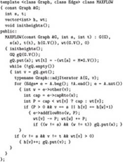
Program 22.5 Preflow-push maxflow implementation
This implementation of the generic vertex-based–preflow-push maxflow algorithm uses a generalized queue that disallows duplicates for active nodes. The wt vector contains each vertex’s excess flow and therefore implicitly defines the set of active vertices. By convention, s is initially active but never goes back on the queue and t is never active. The main loop chooses an active vertex v, then pushes flow through each of its eligible edges (adding vertices that receive the flow to the active list, if necessary), until either v becomes inactive or all its edges have been considered. In the latter case, v’s height is incremented and it goes back onto the queue.
analysis of algorithms and data structures that we examine in more detail in Part 8.
Define the quantity ϕ to be 0 if there are no active vertices and to be the maximum height of the active vertices otherwise, then consider the effect of each phase on the value of ϕ. Let h0(s) be the initial height of the source. At the beginning, ϕ =h0(s); at the end, ϕ =0.
First, we note that the number of phases where the height of some vertex increases is no more than 2V2−h0(s), since each of the V vertex heights can be increased to a value of at most 2V, by the corollary to Property 22.11. Since ϕ can increase only if the height of some vertex increases, the number of phases where ϕ increases is no more than 2V2− h0(s).
If, however, no vertex’s height is incremented during a phase, then ϕ must decrease by at least 1, since the effect of the phase was to push all excess flow from each active vertex to vertices that have smaller height.
Together, these facts imply that the number of phases must be less than 4V2: The value of ϕ is h0(s) at the beginning and can be incremented at most 2V2−h0(s) times and therefore can be decremented at most 2V2 times. The worst case for each phase is that all vertices are on the queue and all of their edges are examined, leading to the stated bound on the total running time.
This bound is tight. Program 22.29 illustrates a family of flow networks for which the number of phases used by the preflow-push algorithm is proportional to V2.
Because our implementations maintain an implicit representation of the residual network, they examine edges leaving a vertex even when those edges are not in the residual network (to test whether or not they are there). It is possible to show that we can reduce the bound in Property 22.13 from V2E to V3 for an implementation that eliminates this cost by maintaining an explicit representation of the residual network. Although the theoretical bound is the lowest that we have seen for the maxflow problem, this change may not be worth the trouble, particularly for the sparse graphs that we see in practice (see Exercises 22.63 through 22.65).
Again, these worst-case bounds tend to be pessimistic and thus not necessarily useful for predicting performance on real networks (though the gap is not as excessive as we found for augmenting-path
Figure 22.29 FIFO preflow-push worst case
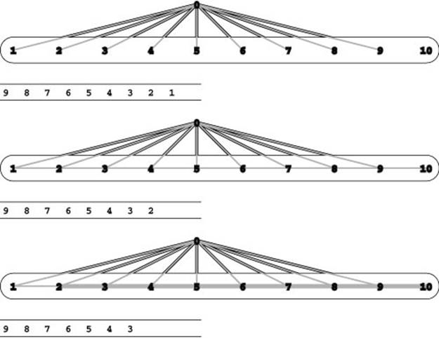
This network represents a family of networks with V vertices such that the total running time of the preflow-push algorithm is proportional to V2. It consists of unit-capacity edges emanating from the source (vertex 0) and horizontal edges of capacity v− 2 running from left to right towards the sink (vertex 10). In the initial phase of the preflow-push algorithm (top), we push one unit of flow out each edge from the source, making all the vertices active except the source and the sink. In a standard adjacency-lists representation, they appear on the FIFO queue of active vertices in reverse order, as shown below the network. In the second phase (center), we push one unit of flow from 9 to 10, making 9 inactive (temporarily); then we push one unit of flow from 8 to 9, making 8 inactive (temporarily) and making 9 active; then we push one unit of flow from 7 to 8, making 7 inactive (temporarily) and making 8 active; and so forth. Only 1 is left inactive. In the third phase (bottom), we go through a similar process to make 2 inactive, and the same process continues for V − 2 phases.
algorithms). For example, the FIFO algorithm finds the flow in the network illustrated in Program 22.30 in 15 phases, whereas the bound in the proof of Property 22.13 says only that it must do so in fewer than 182.
To improve performance, we might try using a stack, a randomized queue, or any other generalized queue in Program 22.5. One approach that has proved to do well in practice is to implement the generalized queue such that GQget returns the highest active vertex. We refer to this method as the highest-vertex–preflow-push maxflow algorithm. We can implement this strategy with a priority queue, although it is also possible to take advantage of the particular properties of heights to implement the generalized-queue operations in constant time. A worst-case time bound of V2 ![]() (which is V5/2 for sparse graphs) has been proved for this algorithm (see reference section); as usual, this bound is pessimistic. Many other preflow-push variants have been proposed, several of which reduce the worst-case time bound to be close to V E (see reference section).
(which is V5/2 for sparse graphs) has been proved for this algorithm (see reference section); as usual, this bound is pessimistic. Many other preflow-push variants have been proposed, several of which reduce the worst-case time bound to be close to V E (see reference section).
Table 22.2 shows performance results for preflow-push algorithms corresponding to those for augmenting-path algorithms in Table
Figure 22.30 Preflow-push algorithm (FIFO)
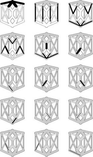
This sequence illustrates how the FIFO implementation of the preflow-push method finds a maximum flow in a sample network. It proceeds in phases: First it pushes as much flow as it can from the source along the edges leaving the source (top left). Then, it pushes flow from each of those nodes, continuing until all nodes are in equilibrium.
Table 22.2 Empirical study of preflow-push algorithms
This table shows performance parameters (number of vertices expanded and number of adjacency-list nodes touched) for various preflow-push network-flow algorithms for our sample Euclidean neighbor network (with random capacities with maxflow value 286) and with unit capacities (with maxflow value 6). Differences among the methods are minimal for both types of networks. For random capacities, the number of edges examined is about the same as for the random augmenting-path algorithm (see Table 22.1). For unit capacities, the augmenting-path algorithms examine substantially fewer edges for these networks.
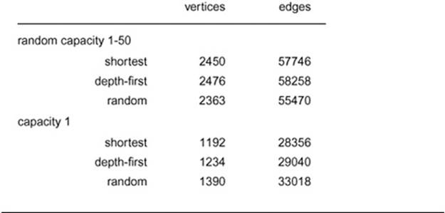
22.1, for the two network models discussed in Section 22.2. These experiments show much less performance variation for the various preflow-push methods than we observed for augmenting-path methods.
There are many options to explore in developing preflow-push implementations. We have already discussed three major choices:
• Edge-based versus vertex-based generic algorithm
• Generalized queue implementation
• Initial assignment of heights
There are several other possibilities to consider and many options to try for each, leading to a multitude of different algorithms to study (see, for example, Exercises 22.56 through 22.60). The dependence of an algorithm’s performance on characteristics of the input network further multiplies the possibilities.
The two generic algorithms that we have discussed (augmenting-path and preflow-push) are among the most important from an extensive research literature on maxflow algorithms. The quest for better maxflow algorithms is still a potentially fruitful area for further research. Researchers are motivated to develop and study new algorithms and implementations by the reality of faster algorithms for practical problems and by the possibility that a simple linear algorithm exists for the maxflow problem. Until one is discovered, we can work confidently with the algorithms and implementations that we have discussed; numerous studies have shown them to be effective for a broad range of practical maxflow problems.
Exercises
• 22.49 Describe the operation of the preflow-push algorithm in a network whose capacities are in equilibrium.
22.50 Use the concepts described in this section (height functions, eligible edges, and pushing of flow through edges) to describe augmenting-path maxflow algorithms.
22.51 Show, in the style of Program 22.28, the flow and residual networks after each phase when you use the FIFO preflow-push algorithm to find a maxflow in the flow network shown in Program 22.10.
• 22.52 Implement the initheights() function for Program 22.5, using breadth-first search from the sink.
22.53 Do Exercise 22.51 for the highest-vertex–preflow-push algorithm.
• 22.54 Modify Program 22.5 to implement the highest-vertex–preflow-push algorithm, by implementing the generalized queue as a priority queue. Run empirical tests so that you can add a line to Table 22.2 for this variant of the algorithm.
22.55 Plot the number of active vertices and the number of vertices and edges in the residual network as the FIFO preflow-push algorithm proceeds, for specific instances of various networks (see Exercises 22.7–12).
• 22.56 Implement the generic edge-based–preflow-push algorithm, using a generalized queue of eligible edges. Run empirical studies for various networks (see Exercises 22.7–12) to compare these to the basic methods, studying generalized-queue implementations that perform better than others in more detail.
22.57 Modify Program 22.5 to recalculate the vertex heights periodically to be shortest-path lengths to the sink in the residual network.
• 22.58 Evaluate the idea of pushing excess flow out of vertices by spreading it evenly among the outgoing edges, rather than perhaps filling some and leaving others empty.
22.59 Run empirical tests to determine whether the shortest-paths computation for the initial height function is justified in Program 22.5 by comparing its performance as given for various networks (see Exercises 22.7–12) with its performance when the vertex heights are just initialized to zero.
• 22.60 Experiment with hybrid methods involving combinations of the ideas above. Run empirical studies for various networks (see Exercises 22.7–12) to compare these to the basic methods, studying variations that perform better than others in more detail.
22.61 Modify the implementation of Program 22.5 such that it explicitly disallows duplicate vertices on the generalized queue. Run empirical tests for various networks (see Exercises 22.7–12) to determine the effect of your modification on actual running times.
22.62 What effect does allowing duplicate vertices on the generalized queue have on the worst-case running-time bound of Property 22.13?
22.63 Modify the implementation of Program 22.5 to maintain an explicit representation of the residual network.
• 22.64 Sharpen the bound in Property 22.13 to O (V3) for the implementation of Exercise 22.63. Hint: Prove separate bounds on the number of pushes that correspond to deletion of edges in the residual network and on the number of pushes that do not result in full or empty edges.
22.65 Run empirical studies for various networks (see Exercises 22.7–12) to determine the effect of using an explicit representation of the residual network (see Exercise 22.63) on actual running times.
22.66 For the edge-based generic preflow-push algorithm, prove that the number of pushes that correspond to deleting an edge in the residual network is less than 2V E. Assume that the implementation keeps an explicit representation of the residual network.
• 22.67 For the edge-based generic preflow-push algorithm, prove that the number of pushes that do not correspond to deleting an edge in the residual network is less than 4V2(V + E ). Hint: Use the sum of the heights of the active vertices as a potential function.
• 22.68 Run empirical studies to determine the actual number of edges examined and the ratio of the running time to V for several versions of the preflow-push algorithm for various networks (see Exercises 22.7–12). Consider various algorithms described in the text and in the previous exercises, and concentrate on those that perform the best on huge sparse networks. Compare your results with your result from Exercise 22.34.
• 22.69 Write a client program that does dynamic graphical animations of preflow-push algorithms. Your program should produce images like Program 22.30 and the other figures in this section (see Exercise 22.48). Test your implementation for the Euclidean networks among Exercises 22.7–12.
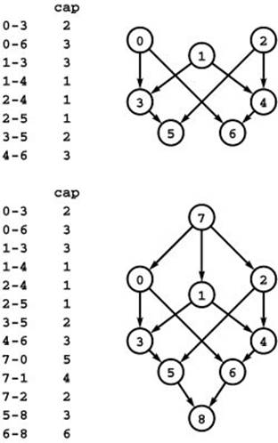
Figure 22.31 Reduction from multiple sources and sinks
The network at the top has three sources (0, 1, and 2) and two sinks (5 and 6). To find a flow that maximizes the total flow out of the sources and into the sinks, we find a maxflow in the st-network illustrated at the bottom. This network is a copy of the original network, with the addition of a new source 7 and a new sink 8. There is an edge from 7 to each original-network source with capacity equal to the sum of the capacities of that source’s outgoing edges, and an edge from each original-network sink to 8 with capacity equal to the sum of the capacities of that sink’s incoming edges.