Algorithms Third Edition in C++ Part 5. Graph Algorithms (2006)

CHAPTER TWENTY-TWO
Network Flow

22.4 Maxflow Reductions

In this section, we consider a number of reductions to the maxflow problem in order to demonstrate that the maxflow algorithms of Sections 22.2 and 22.3 are important in a broad context. We can remove various restrictions on the network and solve other flow problems; we can solve other network- and graph-processing problems; and we can solve problems that are not network problems at all. This section is devoted to examples of such uses—to establish maxflow as a general problem-solving model.

We also consider relationships between the maxflow problem and problems that are more difficult so as to set the context for considering those problems later on. In particular, we note that the maxflow problem is a special case of the mincost-flow problem that is the subject of Sections 22.5and 22.6, and we describe how to formulate maxflow problems as LP problems, which we will address in Part 8. Mincost flow and LP represent problem-solving models that are more general than the maxflow model. Although we normally can solve maxflow problems more easily with the specialized algorithms of Sections 22.2 and 22.3 than with algorithms that solve these more general problems, it is important to be cognizant of the relationships among problem-solving models as we progress to more powerful ones.

We use the term standard maxflow problem to refer to the version of the problem that we have been considering (maxflow in edge-capacitated st-networks). This usage is solely for easy reference in this section. Indeed, we begin by considering reductions that show the restrictions in the standard problem to be essentially immaterial, because several other flow problems reduce to or are equivalent to the standard problem. We could adopt any of the equivalent problems as the “standard” problem. A simple example of such a problem, already noted as a consequence of Property 22.1, is that of finding a circulation in a network that maximizes the flow in a specified edge. Next, we consider other ways to pose the problem, in each case noting its relationship to the standard problem.

Maxflow in general networks Find the flow in a network that maximizes the total outflow from its sources (and therefore the total inflow to its sinks). By convention, define the flow to be zero if there are no sources or no sinks.

Property 22.14 The maxflow problem for general networks is equivalent to the maxflow problem for st-networks.

Proof: A maxflow algorithm for general networks will clearly work for st-networks, so we just need to establish that the general problem reduces to the st-network problem. To do so, first find the sources and sinks (using, for example, the method that we used to initialize the queue in Program 19.8), and return zero if there are none of either. Then, add a dummy source vertex s and edges from s to each source in the network (with each such edge’s capacity set to that edge’s destination vertex’s outflow) and a dummy sink vertex t and edges from each sink in the network to t (with each such edge’s capacity set to that edge’s source vertex’s inflow) Program 22.31 illustrates this reduction. Any maxflow in the st-network corresponds directly to a maxflow in the original network.

Vertex-capacity constraints Given a flow network, find a maxflow satisfying additional constraints specifying that the flow through each vertex must not exceed some fixed capacity.

Property 22.15 The maxflow problem for flow networks with capacity constraints on vertices is equivalent to the standard maxflow problem.

Proof: Again, we could use any algorithm that solves the capacity-constraint problem to solve a standard problem (by setting capacity constraints at each vertex to be larger than its inflow or outflow), so we need only to show a reduction to the standard problem. Given a flow network with capacity constraints, construct a standard flow network with two vertices u and u* corresponding to each original vertex u, with all incoming edges to the original vertex going to u, all outgoing edges coming from u*, and an edge u-u* of capacity equal to the vertex capacity. This construction is illustrated in Program 22.32. The flows in the edges of the form u*-v in any maxflow for the transformed network give a maxflow for the original network that must satisfy the vertex-capacity constraints because of the edges of the form u-u*.

Figure 22.32 Removing vertex capacities

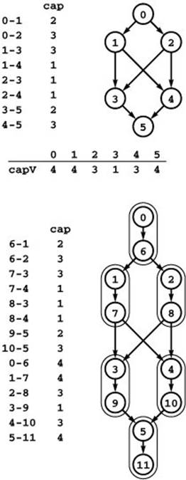
To solve the problem of finding a maxflow in the network at the top such that flow through each vertex does not exceed the capacity bound given in the vertex-indexed array capV, we build the standard network at the bottom: Associate a new vertex u* (where u* denotes u+V) with each vertex u, add an edge u-u* whose capacity is the capacity of u, and include an edge u*-v for each edge u-v. Each u-u* pair is encircled in the diagram. Any flow in the bottom network corresponds directly to a flow in the top network that satisfies the vertex-capacity constraints.

Allowing multiple sinks and sources or adding capacity constraints seem to generalize the maxflow problem; the interest of Properties 22.14 and 22.15 is that these problems are actually no more difficult than the standard problem. Next, we consider a version of the problem that might seem to be easier to solve.

Acyclic networks Find a maxflow in an acyclic network. Does the presence of cycles in a flow network make more difficult the task of computing a maxflow?

We have seen many examples of digraph-processing problems that are much more difficult to solve in the presence of cycles. Perhaps the most prominent example is the shortest-paths problem in weighted digraphs with edge weights that could be negative (see Section 21.7), which is simple to solve in linear time if there are no cycles but NP-complete if cycles are allowed. But the maxflow problem, remarkably, is no easier for acyclic networks.

Property 22.16 The maxflow problem for acyclic networks is equivalent to the standard maxflow problem.

Proof: Again, we need only to show that the standard problem reduces to the acyclic problem. Given any network with V vertices and E edges, we construct a network with 2V +2 vertices and E +3V edges that is not just acyclic but has a simple structure.

Let u* denote u+V, and build a bipartite digraph consisting of two vertices u and u* corresponding to each vertex u in the original network and one edge u-v* corresponding to each edge u-v in the original network with the same capacity. Now, add to the bipartite digraph a source s and a sink t and, for each vertex u in the original graph, an edge s-u and an edge u*-t, both of capacity equal to the sum of the capacities of u’s outgoing edges in the original network. Also, let X be the sum of the capacities of the edges in the original network, and add edges from u to u*, with capacity X+1. This construction is illustrated in Program 22.33.

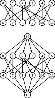
Figure 22.33 Reduction to acyclic network

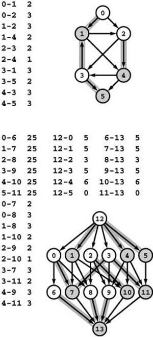
Each vertex u in the top network corresponds to two vertices u and u* (where u* denotes u+V) in the bottom network and each edge u-v in the top network corresponds to an edge u-v* in the bottom network. Additionally, the bottom network has uncapacitated edges u-u*, a source s with an edge to each unstarred vertex, and a sink t with an edge from each starred vertex. The shaded and un-shaded vertices (and edges which connect shaded to unshaded) illustrate the direct relationship among cuts in the two networks (see text).

To show that any maxflow in the original network corresponds to a maxflow in the transformed network, we consider cuts rather than flows. Given any st-cut of size c in the original network, we show how to construct an st-cut of size c+ X in the transformed network; and, given any minimalst-cut of size c+ X in the transformed network, we show how to construct an st-cut of size c in the original network. Thus, given a minimal cut in the transformed network, the corresponding cut in the original network is minimal. Moreover, our construction gives a flow whose value is equal to the minimal-cut capacity, so it is a maxflow.

Given any cut of the original network that separates the source from the sink, let S be the source’s vertex set and T the sink’s vertex set. Construct a cut of the transformed network by putting vertices in S in a set with s and vertices in T in a set with t and putting u and u* on the same side of the cut for all u, as illustrated in Program 22.33. For every u, either s-u or P|u*-t| is in the cut set, and u-v* is in the cut set if and only if u-v is in the cut set of the original network; so the total capacity of the cut is equal to the capacity of the cut in the original network plus X.

Given any minimal st-cut of the transformed network, let S* be s’s vertex set and T*t’s vertex set. Our goal is to construct a cut of the same capacity with u and u* both in the same cut vertex set for all u so that the correspondence of the previous paragraph gives a cut in the original network, completing the proof. First, if u is in S and u* in T*, then u-u* must be a crossing edge, which is a contradiction: u-u* cannot be in any minimal cut, because a cut consisting of all the edges corresponding to the edges in the original graph is of lower cost. Second, if u is in T and u* is in S, then s-u must be in the cut, because that is the only edge connecting s to u. But we can create a cut of equal cost by substituting all the edges directed out of u for s-u, moving u to S*.

Given any flow in the transformed network of value c + X, we simply assign the same flow value to each corresponding edge in the original network to get a flow with value c. The cut transformation at the end of the previous paragraph does not affect this assignment, because it manipulates edges with flow value zero.

The result of the reduction not only is an acyclic network, but also has a simple bipartite structure. The reduction says that we could, if we wished, adopt these simpler networks, rather than general networks, as our standard. It would seem that perhaps this special structure would lead to faster maxflow algorithms. But the reduction shows that we could use any algorithm that we found for these special acyclic networks to solve maxflow problems in general networks, at only modest extra cost. Indeed, the classical maxflow algorithms exploit the flexibility of the general network model: Both the augmenting-path and preflow-push approaches that we have considered use the concept of a residual network, which involves introducing cycles into the network.

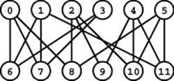
Figure 22.34 Reduction from undirected networks

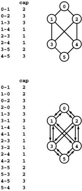
To solve a maxflow problem in an undirected network, we can consider it to be a directed network with edges in each direction. Note that the residual network for such a network has four edges corresponding to each edge in the undirected network.

When we have a maxflow problem for an acyclic network, we typically use the standard algorithm for general networks to solve it.

The construction of Property 22.16 is elaborate, and it illustrates that reduction proofs can require care, if not ingenuity. Such proofs are important because not all versions of the maxflow problem are equivalent to the standard problem, and we need to know the extent of the applicability of our algorithms. Researchers continue to explore this topic because reductions relating various natural problems have not yet been established, as illustrated by the following example.

Maxflow in undirected networks An undirected flow network is a weighted graph with integer edge weights that we interpret to be capacities. A circulation in such a network is an assignment of weights and directions to the edges satisfying the conditions that the flow on each edge is no greater than that edge’s capacity and that the total flow into each vertex is equal to the total flow out of that vertex. The undirected maxflow problem is to find a circulation that maximizes the flow in specified direction in a specified edge (that is, from some vertex s to some other vertex t). This problem perhaps corresponds more naturally than the standard problem to our liquid-flowing-through-pipes model: It corresponds to allowing liquid to flow through a pipe in either direction.

Property 22.17 The maxflow problem for undirected st-networks reduces to the maxflow problem for st-networks.

Proof: Given an undirected network, construct a directed network with the same vertices and two directed edges corresponding to each edge, one in each direction, both with the capacity of the undirected edge. Any flow in the original network certainly corresponds to a flow with the same value in the transformed network. The converse is also true: If u-v has flow f and v-u flow g in the undirected network, then we can put the flow f − g in u-v in the directed network if f≥g; g −f in v-u otherwise. Thus, any maxflow in the directed network is a maxflow in the undirected network: The construction gives a flow, and any flow with a higher value in the directed network would correspond to some flow with a higher value in the undirected network; but no such flow exists.

This proof does not establish that the problem for undirected networks is equivalent to the standard problem. That is, it leaves open

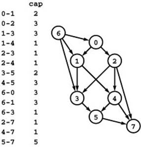
Figure 22.35 Feasible flow

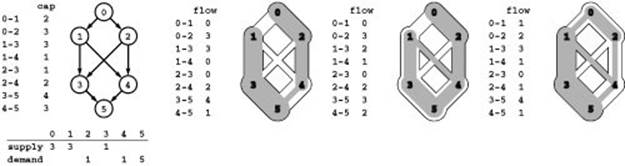
In a feasible-flow problem, we specify supply and demand constraints at the vertices in addition to the capacity constraints on the edges. We seek any flow for which outflow equals supply plus inflow at supply vertices and inflow equals outflow plus demand at demand vertices. Three solutions to the feasible-flow problem at left are shown on the right.

the possibility that finding maxflows in undirected networks is easier than finding maxflows in standard networks (see Exercise 22.81).

In summary, we can handle networks with multiple sinks and sources, undirected networks, networks with capacity constraints on vertices, and many other types of networks (see, for example, Exercise 22.79) with the maxflow algorithms for st-networks in the previous two sections. In fact, Property 22.16 says that we could solve all these problems with even an algorithm that works for only acyclic networks.

Next, we consider a problem that is not an explicit maxflow problem but that we can reduce to the maxflow problem and therefore solve with maxflow algorithms. It is one way to formalize a basic version of the merchandise-distribution problem described at the beginning of this chapter.

Feasible flow Suppose that a weight is assigned to each vertex in a flow network, and is to be interpreted as supply (if positive) or demand (if negative), with the sum of the vertex weights equal to zero. Define a flow to be feasible if the difference between each vertex’s outflow and inflow is equal to that vertex’s weight (supply if positive and demand if negative). Given such a network, determine whether or not a feasible flow exists. Program 22.35 illustrates a feasible-flow problem.

Supply vertices correspond to warehouses in the merchandise-distribution problem; demand vertices correspond to retail outlets; and edges correspond to roads on the trucking routes. The feasible-flow problem answers the basic question of whether it is possible to find a way to ship the goods such that supply meets demand everywhere.

Program 22.6 Feasible flow via reduction to maxflow

This class solves the feasible-flow problem by reduction to maxflow, using the construction illustrated in Program 22.36. The constructor takes as argument a network and a vertex-indexed vector sd such that sd[i] represents, if it is positive, the supply at vertex i and, if it is negative, the demand at vertex i.

As indicated in Program 22.36, the constructor makes a new graph with the same edges but with two extra vertices s and t, with edges from s to the supply nodes and from the demand nodes to t Then it finds a maxflow and checks whether all the extra edges are filled to capacity.

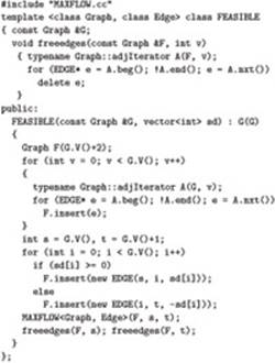
Figure 22.36 Reduction from feasible flow

This network is a standard network constructed from the feasible-flow problem in Program 22.35 by adding edges from a new source vertex to the supply vertices (each with capacity equal to the amount of the supply) and edges to a new sink vertex from the demand vertices (each with capacity equal to the amount of the demand). The network in Program 22.35 has a feasible flow if and only if this network has a flow (a maxflow) that fills all the edges from the sink and all the edges to the source.

Property 22.18 The feasible-flow problem reduces to the maxflow problem.

Proof: Given a feasible-flow problem, construct a network with the same vertices and edges but with no weights on the vertices. Instead, add a source vertex s that has an edge to each supply vertex with weight equal to that vertex’s supply and a sink vertex t that has an edge from each demand vertex with weight equal to the negation of that vertex’s demand (so that the edge weight is positive). Solve the maxflow problem on this network. The original network has a feasible flow if and only if all the edges out of the source and all the edges into the sink are filled to capacity in this flow. Program 22.36 illustrates an example of this reduction.

Developing classes that implement reductions of the type that we have been considering can be a challenging software-engineering task, primarily because the objects that we are manipulating are represented with complicated data structures. To reduce another problem to a standard maxflow problem, should we create a new network? Some of the problems require extra data, such as vertex capacities or supply and demand, so creating a standard network without these data might be justified. Our use of edge pointers plays a critical role here: If we copy a network’s edges and then compute a maxflow, what are we to do with the result? Transferring the computed flow (a weight on each edge) from one network to another when both are represented with adjacency lists is not a trivial computation. With edge pointers, the new network has copies of pointers, not edges, so we can transfer flow assignments right through to the client’s network. Program 22.6 is an implementation that illustrates some of these considerations in a class for solving feasible-flow problems using the reduction of Property 22.16.

A canonical example of a flow problem that we cannot handle with the maxflow model, and that is the subject of Sections 22.5 and 22.6, is an extension of the feasible-flow problem. We add a second set of edge weights that we interpret as costs, define flow costs in terms of these weights, and ask for a feasible flow of minimal cost. This model formalizes the general merchandise-distribution problem. We are interested not just in whether it is possible to move the goods but also in what is the lowest-cost way to move them.

All the problems that we have considered so far in this section have the same basic goal (computing a flow in a flow network), so it is perhaps not surprising that we can handle them with a flow-network problem-solving model. As we saw with the maxflow–mincut theorem, we can use maxflow algorithms to solve graph-processing problems that seem to have little to do with flows. We now turn to examples of this kind.

Maximum-cardinality bipartite matching Given a bipartite graph, find a set of edges of maximum cardinality such that each vertex is connected to at most one other vertex.

For brevity, we refer to this problem simply as the bipartite-matching problem except in contexts where we need to distinguish it from similar problems. It formalizes the job-placement problem discussed at the beginning of this chapter. Vertices correspond to individuals and employers; edges correspond to a “mutual interest in the job” relation. A solution to the bipartite-matching problem maximizes total employment. Program 22.37 illustrates the bipartite graph that models the example problem in Program 22.3.

Figure 22.37 Bipartite matching

This instance of the bipartite-matching problem formalizes the job-placement example depicted in Program 22.3. Finding the best way to match the students to the jobs in that example is equivalent to finding the maximum number of vertex-disjoint edges in this bipartite graph.

It is an instructive exercise to think about finding a direct solution to the bipartite-matching problem, without using the graph model. For example, the problem amounts to the following combinatorial puzzle: “Find the largest subset of a set of pairs of integers (drawn from disjoint sets) with the property that no two pairs have the same integer.” The example depicted in Program 22.37 corresponds to solving this puzzle on the pairs 0-6, 0-7, 0-8, 1-6, and so forth. The problem seems straightforward at first, but, as was true of the Hamilton-path problem that we considered inSection 17.7 (and many other problems), a naive approach that chooses pairs in some systematic way until finding a contradiction might require exponential time. That is, there are far too many subsets of the pairs for us to try all possibilities; a solution to the problem must be clever enough to examine only a few of them. Solving specific matching puzzles like the one just given or developing algorithms that can solve efficiently any such puzzle are nontrivial tasks that help to demonstrate the power and utility of the network-flow model, which provides a reasonable way to do bipartite matching.

Property 22.19 The bipartite-matching problem reduces to the maxflow problem.

Proof: Given a bipartite-matching problem, construct an instance of the maxflow problem by directing all edges from one set to the other, adding a source vertex with edges directed to all the members of one set in the bipartite graph, and adding a sink vertex with edge directed from all the members of the other set. To make the resulting digraph a network, assign each edge capacity 1. Program 22.38 illustrates this construction.

Now, any solution to the maxflow problem for this network provides a solution to the corresponding bipartite-matching problem. The matching corresponds exactly to those edges between vertices in the two sets that are filled to capacity by the maxflow algorithm. First, the network flow always gives a legal matching: Since each vertex has an edge of capacity one either coming in (from the sink) or going out (to the source), at most one unit of flow can go through each vertex, implying in turn that each vertex will be included at most once in the matching. Second, no matching can have more edges, since any such matching would lead directly to a better flow than that produced by the maxflow algorithm.

Figure 22.38 Reduction from bipartite matching

To find a maximum matching in a bipartite graph (top), we construct an st-network (bottom) by directing all the edges from the top row to the bottom row, adding a new source with edges to each vertex on the top row, adding a new sink with edges to each vertex on the bottom row, and assigning capacity 1 to all edges. In any flow, at most one outgoing edge from each vertex on the top row can be filled and at most one incoming edge to each vertex on the bottom row can be filled, so a solution to the maxflow problem on this network gives a maximum matching for the bipartite graph.

For example, in Program 22.38, an augmenting-path maxflow algorithm might use the paths s-0-6-t, s-1-7-t, s-2-8-t, s-4-9-t, s-5-10-t, and s-3-6-0-7-1-11-t to compute the matching 0-7, 1-11, 2-8, 3-6, 4-9, and 5-10. Thus, there is a way to match all the students to jobs in Program 22.3.

Program 22.7 is a client program that reads a bipartite-matching problem from standard input and uses the reduction described in this proof to solve it. What is the running time of this program for huge networks? Certainly, the running time depends on the maxflow algorithm and implementation that we use. Also, we need to take into account that the networks that we build have a special structure (unit-capacity bipartite flow networks)—not only do the running times of the various maxflow algorithms that we have considered not necessarily approach their worst-case bounds, but also we can substantially reduce the bounds. For example, the first bound that we considered, for the generic augmenting-path algorithm, provides a quick answer.

Corollary The time required to find a maximum-cardinality matching in a bipartite graph is O(V E).

Proof: Immediate from Property 22.6.

Program 22.7 Bipartite matching via reduction to maxflow

This client reads a bipartite matching problem with V + V vertices and E edges from standard input, then constructs a flow network corresponding to the bipartite matching problem, finds the maximum flow in the network, and uses the solution to print a maximum bipartite matching.

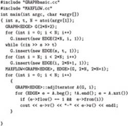
The operation of augmenting-path algorithms on unit-capacity bipartite networks is simple to describe. Each augmenting path fills one edge from the source and one edge into the sink. These edges are never used as back edges, so there are at most V augmenting paths. The V E upper bound holds for any algorithm that finds augmenting paths in time proportional to E.

Table 22.3 shows performance results for solving random bipartite-matching problems using various augmenting-path algorithms. It is clear from this table that actual running times for this problem are closer to the V E worst case than to the optimal (linear)

Table 22.3 Empirical study for bipartite matching

This table shows performance parameters (number of vertices expanded and number of adjacency-list nodes touched) when various augmenting-path maxflow algorithms are used to compute a maximum bipartite matching for graphs with 2000 pairs of vertices and 500 edges (top) and 4000 edges (bottom). For this problem, depth-first search is the most effective method.

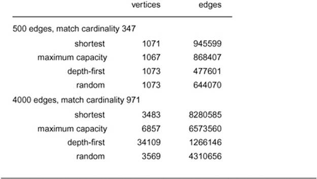
time. It is possible, with judicious choice and tuning of the maxflow implementation, to speed up this method by a factor of pV (see Exercises 22.91 and 22.92).

This problem is representative of a situation that we face more frequently as we examine new problems and more general problem-solving models, demonstrating the effectiveness of reduction as a practical problem-solving tool. If we can find a reduction to a known general model such as the maxflow problem, we generally view that as a major step toward developing a practical solution, because it at least indicates not only that the problem is tractable, but also that we have numerous efficient algorithms for solving the problem. In many situations, it is reasonable to use an existing maxflow class to solve the problem and move on to the next problem. If performance remains a critical issue, we can study the relative performance of various maxflow algorithms or implementations, or we can use their behavior as the starting point to develop a better, special-purpose algorithm.

The general problem-solving model provides both an upper bound that we can choose either to live with or to strive to improve, and a host of implementations that have proved effective on a variety of other problems.

Next, we discuss problems relating to connectivity in graphs. Before considering the use of maxflow algorithms to solve connectivity problems, we examine the use of the maxflow–mincut theorem to take care of a piece of unfinished business from Chapter 18: The proofs of the basic theorems relating to paths and cuts in undirected graphs. These proofs are further testimony to the fundamental importance of the maxflow–mincut theorem.

Property 22.20 (Menger’s Theorem) The minimum number of edges whose removal disconnects two vertices in a digraph is equal to the maximum number of edge-disjoint paths between the two vertices.

Proof: Given a digraph, define a flow network with the same vertices and edges with all edge capacities defined to be 1. By Property 22.2, we can represent any st-flow as a set of edge-disjoint paths from s to t, with the number of such paths equal to the value of the flow. The capacity of anyst-cut is equal to that cut’s cardinality. Given these facts, the maxflow–mincut theorem implies the stated result.

The corresponding results for undirected graphs, and for vertex connectivity for digraphs and for undirected graphs, involve reductions similar to those considered here and are left for exercises (see Exercises 22.94 through 22.96).

Now we turn to algorithmic implications of the direct connection between flows and connectivity that is established by the maxflow– mincut theorem. Property 22.5 is perhaps the most important algorithmic implication (the mincut problem reduces to the maxflow problem), but the converse is not known to be true (see Exercise 22.47). Intuitively, it seems as though knowing a mincut should make easier the task of finding a maxflow, but no one has been able to demonstrate how. This basic example highlights the need to proceed with care when working with reductions among problems.

Still, we can also use maxflow algorithms to handle numerous connectivity problems. For example, they help solve the first nontrivial graph-processing problems that we encountered, in Chapter 18.

Edge connectivity What is the minimum number of edges that need to be removed to separate a given graph into two pieces? Find a set of edges of minimal cardinality that does this separation.

Vertex connectivity What is the minimum number of vertices that need to be removed to separate a given graph into two pieces? Find a set of vertices of minimal cardinality that does this separation.

These problems also are relevant for digraphs, so there are a total of four problems to consider. As with Menger’s theorem, we consider one of them in detail (edge connectivity in undirected graphs) and leave the others for exercises.

Property 22.21 The time required to determine the edge connectivity of an undirected graph is O(E²).

Proof: We can compute the minimum size of any cut that separates two given vertices by computing the maxflow in the st-network formed from the graph by assigning unit capacity to each edge. The edge connectivity is equal to the minimum of these values over all pairs of vertices.

We do not need to do the computation for all pairs of vertices, however. Let s* be a vertex of minimal degree in the graph. Note that the degree of s* can be no greater than 2E/V. Consider any minimum cut of the graph. By definition, the number of edges in the cut set is equal to the graph’s edge connectivity. The vertex s* appears in one of the cut’s vertex sets, and the other set must have some vertex t, so the size of any minimal cut separating s* and t must be equal to the graph’s edge connectivity. Therefore, if we solve V-1 maxflow problems (using s* as the source and each other vertex as the sink), the minimum flow value found is the edge connectivity of the network.

Now, any augmenting-path maxflow algorithm with s* as the source uses at most 2E/V paths; so, if we use any method that takes at most E steps to find an augmenting path, we have a total of at most (V − 1)(2E/V )E steps to find the edge connectivity and that implies the stated result.

This method, unlike all the other examples of this section, is not a direct reduction of one problem to another, but it does give a practical algorithm for computing edge connectivity. Again, with a careful maxflow implementation tuned to this specific problem, we can improve performance—it is possible to solve the problem in time proportional to V E (see reference section). The proof of Property 22.21 is an example of the more general concept of efficient (polynomial-time) reductions that we first encountered in Section 21.7 and that plays an essential role in the theory of algorithms discussed in Part 8. Such a reduction both proves the problem to be tractable and provides an algorithm for solving it—significant first steps in coping with a new combinatorial problem.

We conclude this section by considering a strictly mathematical formulation of the maxflow problem, using linear programming (LP) (see Section 21.6). This exercise is useful because it helps us to see relationships to other problems that can be so formulated.

The formulation is straightforward: We consider a system of inequalities that involve one variable corresponding to each edge, two inequalities corresponding to each edge, and one equation corresponding to each vertex. The value of the variable is the edge flow, the inequalities specify that the edge flow must be between 0 and the edge’s capacity, and the equations specify that the total flow on the edges that go into each vertex must be equal to the total flow on the edges that go out of that vertex.

Figure 22.39 LP formulation of a maxflow problem

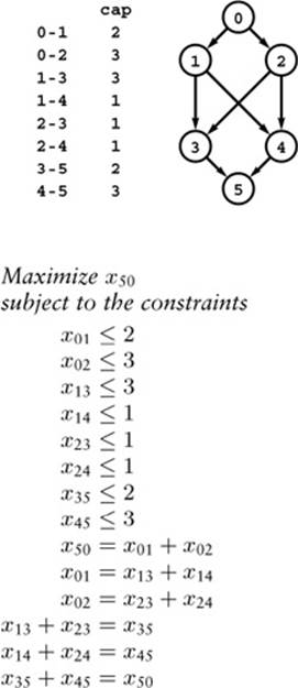
This linear program is equivalent to the maxflow problem for the sample network of Program 22.5. There is one inequality for each edge (which specifies that flow cannot exceed capacity) and one equality for each vertex (which specifies that flow in must equal flow out). We use a dummy edge from sink to source to capture the flow in the network, as described in the discussion following Property 22.2.

Figure 22.39 illustrates an example of this construction. Any maxflow problem can be cast as a LP problem in this way. LP is a versatile approach to solving combinatorial problems, and a great number of the problems that we study can be formulated as linear programs. The fact that maxflow problems are easier to solve than LP problems may be explained by the fact that the constraints in the LP formulation of maxflow problems have a specific structure not necessarily found in all LP problems.

Even though the LP problem is much more difficult in general than are specific problems such as the maxflow problem, there are powerful algorithms that can solve LP problems efficiently. The worst-case running time of these algorithms certainly exceeds the worst-case running of the specific algorithms that we have been considering, but an immense amount of practical experience over the past several decades has shown them to be effective for solving problems of the type that arise in practice.

The construction illustrated in Program 22.39 indicates a proof that the maxflow problem reduces to the LP problem, unless we insist that flow values be integers. When we examine LP in detail in Part 8, we describe a way to overcome the difficulty that the LP formulation does not carry the constraint that the results have integer values.

This context gives us a precise mathematical framework that we can use to address ever more general problems and to create ever more powerful algorithms to solve those problems. The maxflow problem is easy to solve and also is versatile in its own right, as indicated by the examples in this section. Next, we examine a harder problem (still easier than LP) that encompasses a still-wider class of practical problems. We discuss ramifications of building solutions to these increasingly general problem-solving models at the end of this chapter, setting the stage for a full treatment in Part 8.

Exercises

• 22.70 Define a class for finding a circulation with maximal flow in a specified edge. Provide an implementation that uses MAXFLOW.

22.71 Define a class for finding a maxflow in a network with no constraint on the number of sources or sinks. Provide an implementation that uses MAXFLOW.

22.72 Define a class for finding a maxflow in an undirected network. Provide an implementation that uses MAXFLOW.

22.73 Define a class for finding a maxflow in a network with capacity constraints on vertices. Provide an implementation that uses MAXFLOW.

• 22.74 Develop a class for feasible-flow problems that includes member functions allowing clients to set supply–demand values and to check that flow values are properly related at each vertex.

22.75 Do Exercise 22.18 for the case that each distribution point has limited capacity (that is, there is a limit on the amount of goods that can be stored there at any given time).

• 22.76 Show that the maxflow problem reduces to the feasible-flow problem (so that the two problems are therefore equivalent).

22.77 Find a feasible flow for the flow network shown in Program 22.10, given the additional constraints that 0, 2, and 3 are supply vertices with weight 4, andthat 1, 4, and 5 are supply vertices with weights 1, 3, and 5, respectively.

• 22.78 Write a program that takes as input a sports league’s schedule and current standings and determines whether a given team is eliminated. Assume that there are no ties. Hint: Reduce to a feasible-flow problem with one source node that has a supply value equal to the total number of games remaining to play in the season, sink nodes that correspond to each pair of teams having a demand value equal to the number of remaining games between that pair, and distribution nodes that correspond to each team. Edges should connect the supply node to each team’s distribution node (of capacity equal to the number of games that team would have to win to beat X if X were to win all its remaining games), and there should be an (uncapacitated) edge connecting each team’s distribution node to each of the demand nodes involving that team.

• 22.79 Prove that the maxflow problem for networks with lower bounds on edges reduces to the standard maxflow problem.

• 22.80 Prove that, for networks with lower bounds on edges, the problem of finding a minimal flow (that respects the bounds) reduces to the maxflow problem (see Exercise 22.79).

••• 22.81 Prove that the maxflow problem for st-networks reduces to the maxflow problem for undirected networks, or find a maxflow algorithm for undirected networks that has a worst-case running time substantially better than those of the algorithms in Sections 22.2 and 22.3.

• 22.82 Find all the matchings with five edges for the bipartite graph in Program 22.37.

22.83 Extend Program 22.7 to use symbolic names instead of integers to refer to vertices (see Program 17.10).

• 22.84 Prove that the bipartite-matching problem is equivalent to the problem of finding maxflows in networks where all edges are of unit capacity.

22.85 We might interpret the example in Program 22.3 as describing student preferences for jobs and employer preferences for students, the two of which may not be mutual. Does the reduction described in the text apply to the directed bipartite-matching problem that results from this interpretation, where edges in the bipartite graph are directed (in either direction) from one set to the other? Prove that it does or provide a counterexample.

• 22.86 Construct a family of bipartite-matching problems where the average length of the augmenting paths used by any augmenting-path algorithm to solve the corresponding maxflow problem is proportional to E.

22.87 Show, in the style of Program 22.28, the operation of the FIFO preflow-push network-flow algorithm on the bipartite-matching network shown in Program 22.38.

• 22.88 Extend Table 22.3 to include various preflow-push algorithms.

•• 22.89 Suppose that the two sets in a bipartite-matching problem are of size S and T, with S << T. Give as sharp a bound as you can for the worst-case running time to solve this problem, for the reduction of Property 22.19 and the maximal-augmenting-path implementation of the Ford–Fulkerson algorithm (see Property 22.8).

• 22.90 Exercise 22.89 for the FIFO-queue implementation of the preflow-push algorithm (see Property 22.13).

22.91 Extend Table 22.3 to include implementations that use the all-augmenting-paths approach described in Exercise 22.37.

•• 22.92 Prove p that the running time of the method described in Exercise 22.91 is O(E) for BFS.

22.93 Do empirical studies to plot the expected number of edges in a maximal matching in random bipartite graphs with V + V vertices and E edges, for a reasonable set of values for V and sufficient values of E to plot a smooth curve that goes from zero to V.

• 22.94 Prove Menger’s theorem (Property 22.20) for undirected graphs.

• 22.95 Prove that the minimum number of vertices whose removal disconnects two vertices in a digraph is equal to the maximum number of vertex-disjoint paths between the two vertices. Hint: Use a vertex-splitting transformation, similar to the one illustrated in Program 22.32.

• 22.96 Extend your proof for Exercise 22.95 to apply to undirected graphs.

22.97 Implement an edge-connectivity class for the graph ADT of Chapter 17 whose constructor uses the algorithm described in this section to support a public member function that returns the graph’s connectivity.

22.98 Extend your solution to Exercise 22.97 to put in a user-supplied vector a minimal set of edges that separates the graph. How big a vector should the user expect?

• 22.99 Develop an algorithm for computing the edge connectivity of di-graphs (the minimal number of edges whose removal leaves a digraph that is not strongly connected). Implement a class based on your algorithm for the digraph ADT of Chapter 19.

• 22.100 Develop algorithms based on your solutions to Exercises 22.95 and 22.96 for computing the vertex connectivity of digraphs and undirected graphs. Implement classes based on your algorithms for the digraph ADT of Chapter 19 and the graph ADT of Chapter 17, respectively (seeExercises 22.97 and 22.98).

22.101 Describe how to find the vertex connectivity of a digraph by solving V lg V unit-capacity maxflow problems. Hint: Use Menger’s theorem and binary search.

• 22.102 Run empirical studies based on your solution to Exercise 22.97 to determine edge connectivity of various graphs (see Exercises 17.63–76).

• 22.103 Give an LP formulation for the problem of finding a maxflow in the flow network shown in Program 22.10.

• 22.104 Formulate as an LP problem the bipartite-matching problem in Program 22.37.