Discovering Modern C++. An Intensive Course for Scientists, Engineers, and Programmers(2016)

Appendix B. Programming Tools

In this chapter, we introduce some basic programming tools that can help us to achieve our programming goals.

B.1 gcc

One of the most popular C++ compilers is g++, the C++ version of the C compiler gcc. The acronym used to stand for Gnu C Compiler, but the compiler supports several other languages (Fortran, D, Ada, . . .) and the name was changed to Gnu Compiler Collection while keeping the acronym. This section gives a short introduction to how to use it.

The following command:

g++ -o hello hello.cpp

compiles the C++ source file hello.cpp into the executable hello. The flag -o can be omitted. Then the executable will be named a.out (for bizarre historical reasons as an abbreviation of “assembler output”). As soon as we have more than one C++ program in a directory, it will be annoying that executables overwrite each other all the time; thus it is better to use the output flag.

The most important compiler options are

• -I directory: Add directory to include path;

• -O n: Optimize with level n;

• -g: Generate debug information;

• -p: Generate profiling information;

• -o filename: name the output filename instead of a.out;

• -c: Compile only, do not link;

• -L directory: Directory for the next library;

• -D macro: Define macro;

• -l file: Link with library libfile.a or libfile.so.

A little more complex example is

g++ -o myfluxer myfluxer.cpp -I/opt/include -L/opt/lib - lblas

It compiles the file myfluxer.cpp and links it with the BLAS library in directory /opt/lib. Include files are searched in /opt/include in addition to the standard include path.

For generating fast executables, we have to use at least the following flags:

-O3 -DNDEBUG

-O3 is the highest optimization in g++. -DNDEBUG defines a macro that lets assert disappear in the executable by conditional compilation (#ifndef NDEBUG). Disabling assertion is very important for performance: MTL4, for instance, is almost an order of magnitude slower since each access is then range-checked. Conversely, we should use certain compiler flags for debugging as well:

-O0 -g

-O0 turns off all optimizations and globally disables inlining so that a debugger can step through the program. The flag -g lets the compiler store all names of functions and variables and labels of source lines in the binaries so that a debugger can associate the machine code with the source. A short tutorial for using g++ is found at http://tinf2.vub.ac.be/~dvermeir/manual/uintro/gpp.html.

B.2 Debugging

For those of you who play Sudoku, let us dare a comparison. Debugging a program is somewhat similar to fixing a mistake in a Sudoku: it is either quick and easy or really annoying, rarely in between. If the error was made quite recently, we can rapidly detect and fix it. When the mistake remains undetected for a while, it leads to false assumptions and causes a cascade of follow-up errors. As a consequence, in the search for the error we find many parts with wrong results and/or contradictions but which are consistent in themselves. The reason is that they are built on false premises. Questioning everything that we have created before with a lot of thought and work is very frustrating. In the case of a Sudoku, it is often best to ditch it altogether and start all over. For software development, this is not always an option.

Defensive programming with elaborate error handling—not only for user mistakes but for our own potential programming errors as well—not only leads to better software but is also quite often an excellent investment of time. Checking for our own programming errors (with assertions) takes a proportional amount of extra work (say, 5–20 %) whereas the debugging effort can grow infinitely when a bug is hidden deep inside a large program.

B.2.1 Text-Based Debugger

There are several debugging tools. In general, graphical ones are more user-friendly, but they are not always available or usable (especially when working on remote machines). In this section, we describe the gdb debugger, which is very useful to trace back run-time errors.

The following small program using GLAS [29] will serve as a case study:

#include <glas/glas.hpp>
#include <iostream>

int main()
{
glas::dense_vector< int > x( 2 );
x(0)= 1; x(1)= 2;

for (int i= 0; i < 3; ++i)
std::cout x(i) std::endl;
return 0;
}

Running the program in gdb yields the following output:

> gdb myprog
1
2
hello: glas/type/continuous_dense_vector.hpp:85:
T& glas::continuous_dense_vector<T>::operator()(ptrdiff_t) [with T = int]:
Assertion 'i<size_' failed.
Aborted

The reason why the program fails is that we cannot access x(2) because it is out of range. Here is a printout of a gdb session with this program:

(gdb) r
Starting program: hello
1
2
hello: glas/type/continuous_dense_vector.hpp:85:
T& glas::continuous_dense_vector<T>::operator()(ptrdiff_t) [with T = int]:
Assertion 'i<size_' failed.

Program received signal SIGABRT, Aborted.
0xb7ce283b in raise () from /lib/tls/libc.so.6
(gdb) backtrace
#0 0xb7ce283b in raise () from /lib/tls/libc.so.6
#1 0xb7ce3fa2 in abort () from /lib/tls/libc.so.6
#2 0xb7cdc2df in __assert_fail () from /lib/tls/libc.so.6
#3 0x08048c4e in glas::continuous_dense_vector<int>::operator() (
this=0xbfdafe14, i=2) at continuous_dense_vector.hpp:85
#4 0x08048a82 in main () at hello.cpp:10
(gdb) break 7
Breakpoint 1 at 0x8048a67: file hello.cpp, line 7.
(gdb) rerun
The program being debugged has been started already.
Start it from the beginning? (y or n) y
Starting program: hello

Breakpoint 1, main () at hello.cpp:7
7 for (int i=0; i<3; ++i) {
(gdb) step
8 std::cout << x(i) << std::endl ;
(gdb) next
1
7 for (int i=0; i<3; ++i) {
(gdb) next
2
7 for (int i=0; i<3; ++i) {
(gdb) next
8 std::cout << x(i) << std::endl ;
(gdb) print i
$2 = 2
(gdb) next
hello: glas/type/continuous_dense_vector.hpp:85:
T& glas::continuous_dense_vector<T>::operator()(ptrdiff_t) [with T = int]:
Assertion 'i<size_' failed.

Program received signal SIGABRT, Aborted.
0xb7cc483b in raise () from /lib/tls/libc.so.6
(gdb) quit
The program is running. Exit anyway? (y or n) y

The command backtrace tells us where we are in the program. From this back-trace, we can see that the program crashed in line 10 of our main function because an assert was raised in glas::continuous_dense_vector<int>::operator() when i was 2.

B.2.2 Debugging with Graphical Interface: DDD

More convenient than debugging on the text level is using a graphical interface like DDD (Data Display Debugger). It has more or less the same functionality as gdb and in fact it runs gdb internally (or another text debugger). However, we can see our sources and variables as illustrated inFigure B–1.

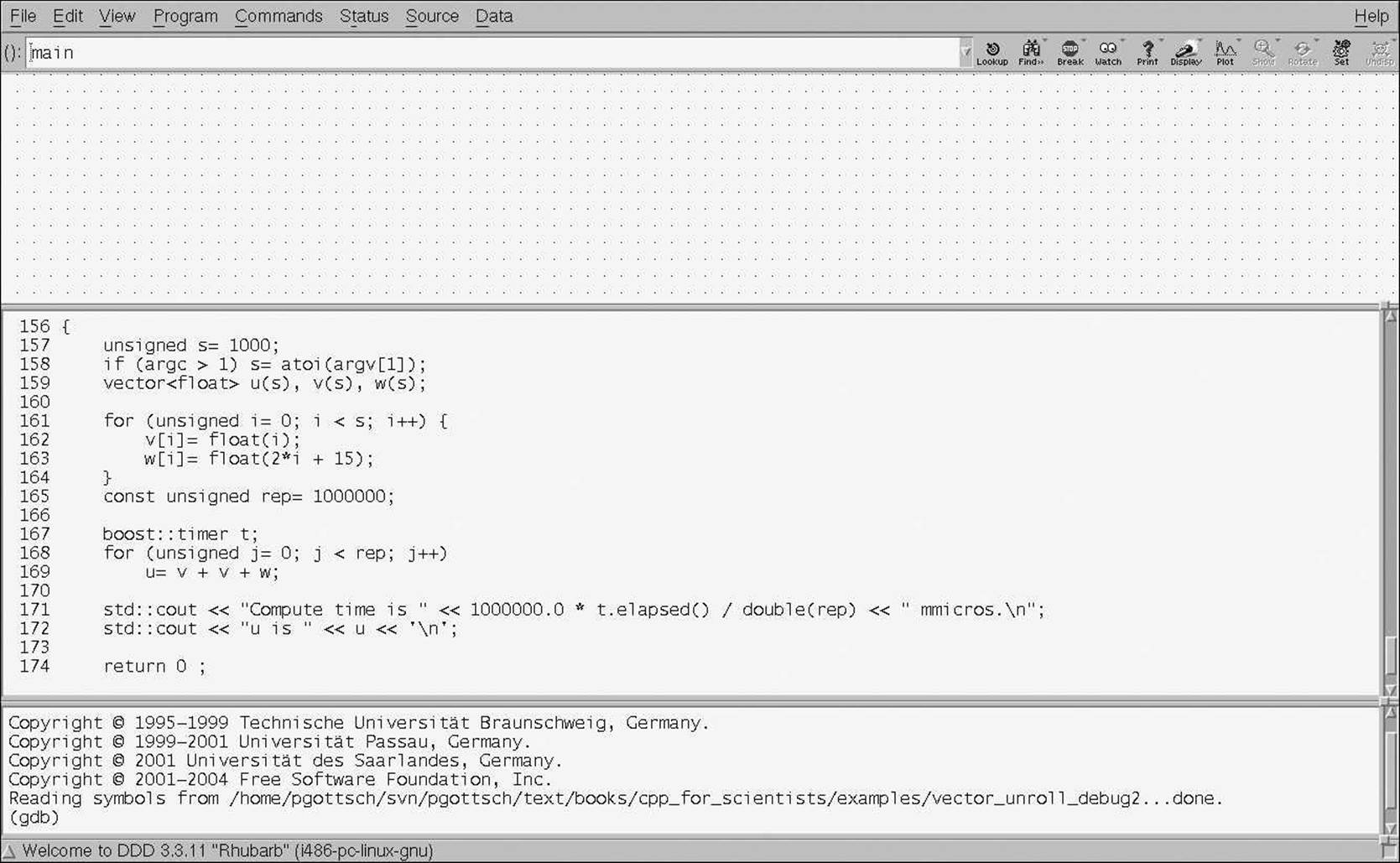
Figure B–1: Debugger window

The screen shot originates from a debugging session of vector_unroll_example2.cpp from Section 5.4.5. In addition to the main window, we see a smaller one like that in Figure B–2, usually on the right of the large window (when there is enough space on the screen). This control panel lets us navigate through the debug session in a way that is easier and more convenient than text debugging. We have the following commands:

Run: Start or restart the program.

Interrupt: If our program does not terminate or does not reach the next break point, we can stop it manually.

Step: Go one step forward. If our position is a function call, jump into the function.

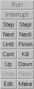
Figure B–2: DDD control panel

Next: Go to the next line in our source code. If we are located on a function call, do not jump into it unless there is a break point set inside.

Stepi and Nexti: This are the equivalents on the instruction level. This is only needed for debugging assembler code.

Until: When we position our cursor in our source, the program runs until it reaches this line. If our program flow does not pass this line, the execution will continue until the end of the program is reached or until the next break point or bug. Alternatively, the program might run eternally in an infinite loop.

Finish: Execute the remainder of the current function and stop in the first line outside this function, i.e., the line after the function call.

Cont: Continue our execution till the next event (break point, bug, or end).

Kill: Kill the program.

Up: Show the line of the current function’s call; i.e., go up one level in the call stack (if available).

Down: Go back to the called function; i.e., go down one level in the call stack (if available).

Undo: Revert the last action (works rarely or never).

Redo: Repeat the last command (works more often).

Edit: Call an editor with the source file currently shown.

Make: Call make to rebuild the executable.

An important new feature in gdb version 7 is the ability to implement pretty printers in Python. This allows us to represent our types concisely in graphical debuggers; for instance, a matrix can be visualized as a 2D array instead of a pointer to the first entry or some other obscure internal representation. IDEs also provide debugging functionality, and some (like Visual Studio) allow for defining pretty printers.

With larger and especially parallel software, it is worthwhile to consider a professional debugger like DDT and Totalview. They allow us to control the execution of a single, some, or all processes, threads, or GPU threads.

B.3 Memory Analysis

c++03/vector_test.cpp

In our experience, the most frequently used tool set for memory problems is the valgrind distribution (which is not limited to memory issues). Here we focus on the memcheck. We apply it to the vector example used, for instance, in Section 2.4.2:

valgrind --tool=memcheck vector_test

memcheck detects memory-management problems like leaks. It also reports read access of uninitialized memory and partly out-of-bounds access. If we omitted the copy constructor of our vector class (so that the compiler would generate one with aliasing effects), we would see the following output:

==17306== Memcheck, a memory error detector
==17306== Copyright (C) 2002-2013, and GNU GPL'd, by Julian Seward et al.
==17306== Using Valgrind-3.10.0.SVN and LibVEX; rerun with -h for copyright info
==17306== Command: vector_test
==17306==
[1,1,2,-3,]
z[3] is -3
w is [1,1,2,-3,]
w is [1,1,2,-3,]
==17306==
==17306== HEAP SUMMARY:
==17306== in use at exit: 72,832 bytes in 5 blocks
==17306== total heap usage: 5 allocs, 0 frees, 72,832 bytes allocated
==17306==
==17306== LEAK SUMMARY:
==17306== definitely lost: 128 bytes in 4 blocks
==17306== indirectly lost: 0 bytes in 0 blocks
==17306== possibly lost: 0 bytes in 0 blocks
==17306== still reachable: 72,704 bytes in 1 blocks
==17306== suppressed: 0 bytes in 0 blocks
==17306== Rerun with --leak-check=full to see details of leaked memory
==17306==
==17306== For counts of detected and suppressed errors, rerun with: -v
==17306== ERROR SUMMARY: 0 errors from 0 contexts (suppressed: 0 from 0)

All these errors can be reported in verbose mode with the corresponding source line and the function stack:

valgrind --tool=memcheck -v --leak-check=full \
--show-leak-kinds=all vector_test

Now we see significantly more details which we refrain from printing here for reasons of size. Please try it on your own.

Program runs with memcheck are slower, in extreme cases up to a factor of 10 or 30. Especially software that uses raw pointers (which hopefully will be an exception in the future) should be checked regularly with valgrind. More information is found at http://valgrind.org.

Some commercial debuggers (like DDT) already contain memory analysis. Visual Studio offers plug-ins for finding memory leaks.

B.4 gnuplot

A public-domain program for visual output is gnuplot. Assume we have a data file results.dat with the following content:

0 1
0.25 0.968713
0.75 0.740851
1.25 0.401059
1.75 0.0953422
2.25 -0.110732
2.75 -0.215106
3.25 -0.237847
3.75 -0.205626
4.25 -0.145718
4.75 -0.0807886
5.25 -0.0256738
5.75 0.0127226
6.25 0.0335624
6.75 0.0397399
7.25 0.0358296
7.75 0.0265507
8.25 0.0158041
8.75 0.00623965
9.25 -0.000763948
9.75 -0.00486465

The first column represents the x-coordinate and the second column contains the corresponding values for u. We can plot these values with the following command in gnuplot:

plot "results.dat" with lines

The command

plot "results.dat"

only plots stars, as depicted in Figure B–3. 3D plots can be realized with the command splot.

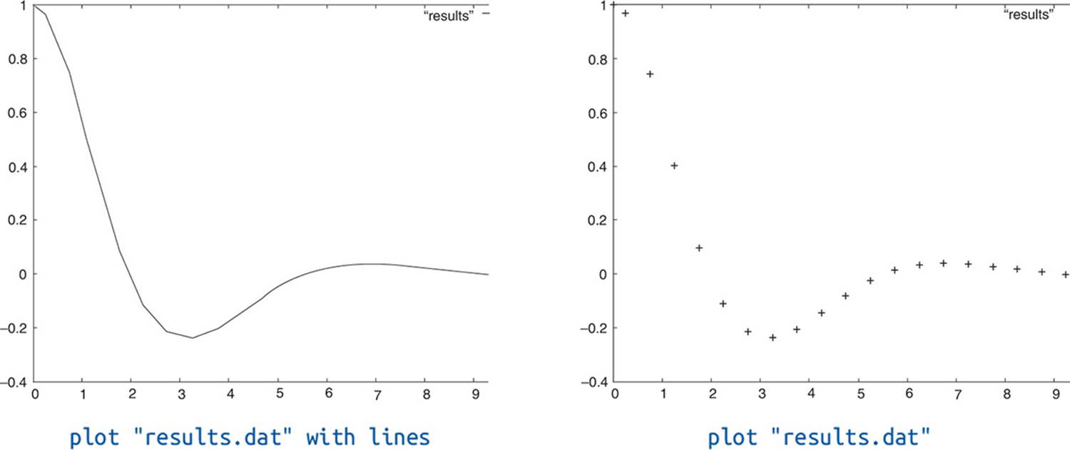
Figure B–3: Plots with plot

For more sophisticated visualization, we can use Paraview which is also freely available.

B.5 Unix, Linux, and Mac OS

Unix systems like Linux and Mac OS provide a rich set of commands that allow us to realize many tasks with little or no programming. Some of the most important commands are:

• ps: List (my) running processes.

• kill id: Kill the process with id id; kill -9 id, force it with signal 9.

• top: List all processes and their resource use.

• mkdir dir: Make a new directory with name dir.

• rmdir dir: Remove an empty directory.

• pwd: Print the current working directory.

• cd dir: Change the working directory to dir.

• ls: List the files in the current directory (or dir).

• cp from to: Copy the file from to the file or directory to. If the file to exists, it is overwritten, unless we use cp -i from to which asks for permission.

• mv from to: Move the file from to directory to if such a directory exists; otherwise rename the file. If the file to exists, it is overwritten. With the flag -i, we are asked for our permission to overwrite files.

• rm files: Remove all the files in the list files. rm * removes everything—be careful.

• chmod mode files: Change the access rights for files.

• grep regex: Find the regular expression regex in the terminal input (or a specified file).

• sort: Sort the input.

• uniq: Filter duplicated lines.

• yes: Write y infinitely or my text with yes 'my text'.

The special charm of Unix commands is that they can be piped; i.e., the output of one program is the input of the next. When we have an installation install.sh for which we are certain that we will respond y to all questions, we can write:

yes | ./install.sh

Or when we want to know all words of length 7 composed of the letters t, i, o, m, r, k, and f :

grep -io '\<[tiomrkf]\{7\}\>' openthesaurus.txt |sort| uniq

This is how the author cheats in the game 4 Pics 1 Word—sometimes.

Of course, we are free to implement similar commands in C++. This is even more efficient when we can combine our programs with system commands. To this end, it is advisable to generate simple output for easier piping. For instance, we can write data that can be processed directly from gnuplot.

More information on Unix commands is found for instance at http://www.physics.wm.edu/unix_intro/outline.html. Obviously, this section is only an appetizer for their power. Likewise, the entire appendix only scratches the surface of the benefits that we can gain from appropriate tools.