Discovering Modern C++. An Intensive Course for Scientists, Engineers, and Programmers(2016)
Appendix A. Clumsy Stuff
This appendix is dedicated to details that cannot be ignored but would slow down the pace we aim for in this book. The early chapters on basics and classes should not hold back the reader from the intriguing advanced topics—at least not longer than necessary. If you would like to learn more details and do not find the sections in this appendix clumsy, the author would not blame you; to the contrary: it would be a pleasure to him. In some sense, this appendix is like the deleted scenes of a movie: they did not make it to the final work but are still valuable to part of the audience.
A.1 More Good and Bad Scientific Software
The goal of this appendix is to give you an idea of what we consider good scientific software and what we do not. Thus, if you do not understand what exactly happens in these programs before reading this book, do not worry. Like the example programs in the Preface, the implementations only provide a first impression of different programming styles in C++ and their pros and cons. The details are not important here, only the general perception and behavior.
As the foundation of our discussion, we consider an iterative method to solve a system of linear equations Ax = b where A is a (sparse) symmetric positive-definite (SPD) matrix, x and b are vectors, and x is searched. The method is called Conjugate Gradients (CG) and was introduced by Magnus R. Hestenes and Eduard Stiefel [24]. The mathematical details do not matter here, but rather the different styles of implementation. The algorithm can be written in the following form:
Algorithm A–1: Conjugate gradient algorithm
Input: SPD matrix A, vector b, and left preconditioner L, termination criterion ![]()
Output: Vector x such that Ax ≈ b
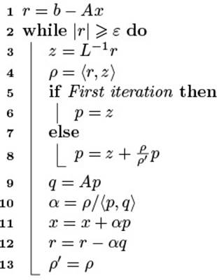
Programmers transform this mathematical notation into a form that a compiler understands by using operations from the language. For those who came here from Chapter 1, we want to introduce our anti-hero Herbert who is an ingenious mathematician and considers programming a necessary evil for demonstrating how magnificently his algorithms work. Implementing other mathematicians’ algorithms is even more annoying to him. His hastily typed version of CG—which you should only skim over—looks like this:
Listing A–1: Low-abstraction implementation of CG
#include <iostream>
#include <cmath>
void diag_prec(int size, double *x, double * y)
{
y[0] = x[0];
for (int i= 1; i < size; i++)
y[i] = 0.5 * x[i];
}
double one_norm(int size, double *vp)
{
double sum= 0;
for (int i= 0; i < size; i++)
sum+= fabs(vp[i]);
return sum;
}
double dot(int size, double *vp, double *wp)
{
double sum= 0;
for (int i= 0; i < size; i++)
sum+= vp[i] * wp[i];
return sum;
}
int cg(int size, double *x, double *b,
void (*prec)(int, double*, double*), double eps)
{
int i, j, iter= 0;
double rho, rho_1, alpha;
double *p= new double[size];
double *q= new double[size];
double *r= new double[size];
double *z= new double[size];
// r= A*x;
r[0] = 2.0 * x[0] - x[1] ;
for (int i= 1; i < size-1; i++)
r[i] = 2.0 * x[i] - x[i-1] - x[i+1];
r[size-1] = 2.0 * x[size-1] - x[size-2];
// r= b-A*x;
for (i= 0; i < size; i++)
r[i]= b[i] - r[i];
while (one_norm (size, r) >= eps) {
prec(size, r, z);
rho= dot(size, r, z);
if (!iter) {
for (i= 0; i < size; i++)
p[i]= z[i];
} else {
for (i= 0; i < size; i++)
p[i]= z[i] + rho / rho_1 * p[i];
}
// q= A * p;
q[0] = 2.0 * p[0] - p[1] ;
for (int i= 1; i < size-1; i++)
q[i] = 2.0 * p[i] - p[i-1] - p[i+1];
q[size-1] = 2.0 * p[size-1] - p[size-2];
alpha= rho / dot(size, p, q);
// x+= alpa * p; r-= alpha * q;
for (i= 0; i < size; i++) {
x[i]+= alpha * p[i];
r[i]-= alpha * q[i];
}
iter ++;
}
delete [] q; delete [] p; delete [] r; delete [] z;
return iter;
}
void ic_0(int size, double* out, double* in) { /* .. */ }
int main (int argc, char* argv[])
{
int size=100;
// set nnz and size
double *x= new double[size];
double *b= new double[size];
for (int i=0; i<size; i++)
b[i] = 1.0 ;
for (int i=0; i<size; i++)
x[i] = 0.0 ;
// set A and b
cg(size, x, b, diag_prec, 1e-9);
return 0 ;
}
Let us discuss it in a general fashion. The good thing about this code is that it is self-contained—a virtue shared with much other bad code. However, this is about the only advantage. The problem with this implementation is its low abstraction level. This creates three major disadvantages:
• Bad readability,
• No flexibility, and
• High proneness to errors.
The bad readability manifests itself in the fact that almost every operation is implemented in one or multiple loops. For instance, would we have found the matrix vector multiplication q = Ap without the comments? Probably. We would easily catch where the variables representing q, A, and pare used, but to see that this is a matrix vector product takes a closer look and a good understanding of how the matrix is stored.
This leads us to the second problem: the implementation commits to many technical details and only works in precisely this context. Algorithm A-1 only requires that matrix A is symmetric positive-definite, but it does not demand a certain storage scheme, even less a specific matrix. Herbert implemented the algorithm for a matrix that represents a discretized 1D Poisson equation. Programming at such a low abstraction level requires modifications every time we have other data or other formats.
The matrix and its format are not the only details the code commits to. What if we want to compute in lower (float) or higher (long double) precision? Or solve a complex linear system? For every such new CG application, we need a new implementation. Needless to say, running on parallel computers or exploring GPGPU (General-Purpose Graphic Processing Units) acceleration needs reimplementations as well. Much worse, every combination of the above needs a new implementation.
Some readers might think: “It is only one function of 20 or 30 lines. Rewriting this little function, how much work can this be? And we do not introduce new matrix formats or computer architectures every month.” Certainly true, but in some sense it is putting the cart before the horse. Because of such inflexible and detail-obsessed programming style, many scientific applications grew into the hundred thousands and millions of lines of code. Once an application or library reaches such a monstrous size, it is arduous to modify features of the software and it is only rarely done. The road to success is starting software from a higher level of abstraction from the beginning, even when it is more work initially.
The last major disadvantage is how prone the code is to errors. All arguments are given as pointers, and the size of the underlying arrays is given as an extra argument. We as programmers of function cg can only hope that the caller did everything right because we have no way to verify it. If the user does not allocate enough memory (or does not allocate it at all), the execution will crash at some more or less random position or, even worse, will generate some nonsensical results because data and even the machine code of our program can be randomly overwritten. Good programmers avoid such fragile interfaces because the slightest mistake can have catastrophic consequences, and the program errors are extremely difficult to locate. Unfortunately, even recently released and widely used software is written in this manner, either for backward compatibility to C and Fortran or because it is written in one of these two languages. Or the developers are just resistant to any progress in software development. In fact, the implementation above is C and not C++. If this is how you like software, you probably will not like this book.
So much about software we do not like. In Listing A–2, we show a version that comes much closer to our ideal.
Listing A–2: High-abstraction implementation of CG
template < typename Matrix, typename Vector,
typename Preconditioner >
int conjugate_gradient(const Matrix& A, Vector& x, const Vector& b,
const Preconditioner& L, const double& eps)
{
typedef typename Collection<Vector>::value_type Scalar;
Scalar rho= 0, rho_1= 0, alpha= 0;
Vector p(resource (x)), q(resource(x)), r(resource(x)),
z(resource(x));
r= b - A * x;
int iter = 0 ;
while (one_norm(size, r) >= eps) {
prec( r, z );
rho = dot(r, z);
if (iter.first())
p = z;
else
p = z + (rho / rho_1) * p;
q= A * p;
alpha = rho / dot (p, q);
x += alpha * p;
r -= alpha * q;
rho_1 = rho;
++iter;
}
return iter;
}
int main (int argc, char* argv[])
{
// initiate A, x, and b
conjugate_gradient(A, x, b, diag_prec, 1. e-5);
return 0 ;
}
The first thing you might realize is that the CG implementation is readable without comments. As a rule of thumb, if other people’s comments look like your program sources, then you are a really good programmer. If you compare the mathematical notation in Algorithm A-1 with Listing A–2 you will realize that—except for the type and variable declarations at the beginning—they are identical. Some readers might think that it looks more like MATLAB or Mathematica than C++. Yes, C++ can look like this if one puts enough effort into good software.
Evidently, it is also much easier to write algorithms at this abstraction level than expressing them with low-level operations.
The Purpose of Scientific Software
Scientists do research. Engineers create new technology.
Excellent scientific and engineering software is expressed only in mathematical and domain-specific operations without any technical detail exposed.
At this abstraction level, scientists can focus on models and algorithms, thus being much more productive and advancing scientific discovery.
Nobody knows how many scientists are wasting how much time every year dwelling on small technical details of bad software like Listing A–1. Of course, the technical details have to be realized in some place but not in a scientific application. This is the worst possible location. Use a two-level approach: write your applications in terms of expressive mathematical operations, and if they do not exist, implement them separately. These mathematical operations must be carefully implemented for absolute correctness and optimal performance. What is optimal depends on how much time you can afford for tuning and on how much benefit the extra performance gives you. Investing time in your fundamental operations pays off when they are reused very often.
Advice
Use the right abstractions!
If they do not exist, implement them.
Speaking of abstractions, the CG implementation in Listing A–2 does not commit to any technical detail. In no place is the function restricted to a numerical type like double. It works as well for float, GNU’s multiprecision, complex, interval arithmetic, quaternions, . . .
The matrix A can be stored in any internal format, as long as A can be multiplied with a vector. In fact, it does not even need to be a matrix but can be any linear operator. For instance, an object that performs a Fast Fourier Transformation (FFT) on a vector can be used as A when the FFT is expressed by a product of A with the vector. Similarly, the vectors do not need to be represented by finite-dimensional arrays but can be elements of any vector space that is somehow computer-representable as long as all operations in the algorithm can be performed.
We are also open to other computer architectures. If the matrix and the vectors are distributed over the nodes of a parallel supercomputer and corresponding parallel operations are available, the function runs in parallel without changing any single line. (GP)GPU acceleration can also be realized without changing the algorithm’s implementation. In general, any existing or new platform for which we can implement matrix and vector types and their corresponding operations is supported by our Generic conjugate gradient function.
As a consequence, sophisticated scientific applications of several thousand lines on top of such abstractions can be ported to new platforms without code modification.
A.2 Basics in Detail
This section accumulates the outsourced details from Chapter 1.
A.2.1 More about Qualifying Literals
Here we want to expand the examples for literal qualifications from Section 1.2.2 a bit.
Availability: The standard library provides a (template) type for complex numbers where the type for the real and imaginary parts can be parameterized by the user:
std::complex<float> z(1.3, 2.4), z2;
These complex numbers of course provide the common operations like addition and multiplication. For unknown reasons, these operations are only provided between the type itself and the underlying real type. Thus, when we write:
z2= 2 * z; // Error: no int * complex<float>
z2= 2.0 * z; // Error: no double * complex<float>
we will get an error message that the multiplication is not available. More specifically, the compiler will tell us that there is no operator*() for int and std::complex<float> respectively for double and std::complex<float>.1 To get the simple expression above compiled, we must make sure that our value 2 has the type float:
1. Since the multiplication is implemented as a template function, the compiler does not convert the int and double to float.
z2= 2.0f * z;
Ambiguity: At some point in this book, we introduced function overloading: a function with different implementations for different argument types (§1.5.4). The compiler selects that function overload which fits best. Sometimes the best fit is not clear, for instance, if function f accepts anunsigned or a pointer and we call:
f(0);
The literal 0 is considered an int and can be implicitly converted into unsigned or any pointer type. None of the conversions is prioritized. As before, we can address the issue by a literal of the desired type:
f(0u);
Accuracy: The accuracy issue comes up when we work with long double. On the author’s computer, the format can handle at least 19 digits. Let us define 1/3 with 20 digits and print out 19 of them:
long double third= 0.3333333333333333333;
cout.precision(19);
cout ![]() "One third is "
"One third is " ![]() third
third ![]() ".\n";
".\n";
The result is
One third is 0.3333333333333333148.
The program behavior is more satisfying if we append an l to the number:
long double third= 0.3333333333333333333l;
yielding the printout that we hoped for:
One third is 0.3333333333333333333.
A.2.2 static Variables
In contrast to the scoped variables from Section 1.2.4 which die at the end of the scope, static variables live till the end of the program. Thus, declaring a local variable as static has an effect only when the contained block is executed more than once: in a loop or a function. Within a function, we could implement a counter for how often the function was called:
void self_observing_function()
{
static int counter= 0; // only executed once
++counter;
cout ![]() "I was called "
"I was called " ![]() counter
counter ![]() " times.\n";
" times.\n";
...
}
To reuse the static data, the initialization is only performed once. The major motivation for static variables is to reuse helper data like lookup tables or caches in the next function call. However, if the management of the helper data reaches a certain complexity, a class-based solution (Chapter 2) probably leads to a cleaner design.
The effect of the keyword static depends on the context but the common denominator is:
• Persistence: data of static variables remains in memory for the rest of the program execution.
• File scope: static variables and functions are only visible in the compilation of the actual file and do not collide when multiple compiled programs are linked together. This is illustrated in Section 7.2.3.2.
Thus, the impact on global variables is to limit their visibility as they already live until the program ends. Conversely, the effect on local variables is the lifetime extension since their visibility is already limited. There is also a class-related meaning of static which is discussed in Chapter 2.
A.2.3 More about if
The condition of an if must be a bool expression (or something convertible to bool). Thus, the following is allowed:
int i= ...
if (i) // bad style
do_something();
This relies on the implicit conversion from int to bool. In other words, we test whether i is different from 0. It is clearer to say this instead:
if (i != 0) // better
do_something();
An if-statement can contain other if-statements:
if (weight > 100.0) {
if (weight > 200.0) {
cout ![]() "This is extremely heavy.\n";
"This is extremely heavy.\n";
} else {
cout ![]() "This is quite heavy.\n";
"This is quite heavy.\n";
}
} else {
if (weight < 50.0) {
cout ![]() "A child can carry this.\n";
"A child can carry this.\n";
} else {
cout ![]() "I can carry this.\n";
"I can carry this.\n";
}
}
In the above example, the parentheses could be omitted without changing the behavior but it is clearer to have them. The example is more readable when we reorganize the nesting:
if (weight < 50.0) {
cout ![]() "A child can carry this.\n";
"A child can carry this.\n";
} else if (weight <= 100.0) {
cout ![]() "I can carry this.\n";
"I can carry this.\n";
} else if (weight <= 200.0) {
cout ![]() "This is quite heavy.\n";
"This is quite heavy.\n";
} else {
cout ![]() "This is extremely heavy.\n";
"This is extremely heavy.\n";
}
The parentheses can be omitted here as well, and it requires less effort to figure out what is going on.
At the end of our discussion on if-then-else, we want to do something sophisticated. Let us take the then-branch of the second-last example without braces:
if (weight > 100.0)
if (weight > 200.0)
cout ![]() "This is extremely heavy.\n";
"This is extremely heavy.\n";
else
cout ![]() "This is quite heavy.\n";
"This is quite heavy.\n";
It looks like the last line is executed when weight is between 100 and 200 assuming the first if has no else-branch. But we could also assume the second if comes without an else-branch and the last line is executed when weight is less than or equal to 100. Fortunately, the C++ standard specifies that an else-branch always belongs to the innermost possible if. So, we can count on our first interpretation. In case the else-branch belongs to the first if we need braces:
if (weight > 100.0) {
if (weight > 200.0)
cout ![]() "This is extremely heavy.\n";
"This is extremely heavy.\n";
} else
cout ![]() "This is not so heavy.\n";
"This is not so heavy.\n";
Maybe these examples will convince you that it is more productive to set more braces and save the time guessing what the branches belong to.
A.2.4 Duff’s Device
The continued execution in switch cases allows us also to implement short loops without the termination test after each iteration. Say we have vectors with dimension ≤ 5. Then we could implement a vector addition without a loop:
assert(size(v) <= 5);
int i= 0;
switch (size(v)) {
case 5: v[i]= w[i] + x[i]; ++i; // keep going
case 4: v[i]= w[i] + x[i]; ++i; // keep going
case 3: v[i]= w[i] + x[i]; ++i; // keep going
case 2: v[i]= w[i] + x[i]; ++i; // keep going
case 1: v[i]= w[i] + x[i]; // keep going
case 0: ;
}
This technique is called Duff’s device. It is usually not used stand-alone as above (but as a cleanup of unrolled loops). Such techniques should not be used in the main development of projects but only as final tuning of performance-critical kernels.
A.2.5 More about main
Arguments containing spaces must be quoted. In the first argument, we can also see when the program is called with path information; e.g.:
../c++11/argc_argv_test first "second third "fourth
prints out:
../c++11/argc_argv_test
first
second third
fourth
Some compilers also support a vector of strings as main arguments. This is more convenient but not portable.
For calculating with the arguments, they must be converted first:
cout ![]() argv[1]
argv[1] ![]() " times "
" times " ![]() argv[2]
argv[2] ![]() " is "
" is "
![]() stof(argv[1]) * stof(argv[2])
stof(argv[1]) * stof(argv[2]) ![]() ".\n";
".\n";
which could provide such impressive knowledge to us:
argc_argv_test 3.9 2.8
3.9 times 2.8 is 10.92.
Unfortunately, the conversion from strings to numbers does not tell us when the complete string is not convertible. As long as the string starts with a number or plus or minus, the reading is stopped if a character is found that cannot belong to a number and the sub-string read up to this point is converted to a number.
In Unix-like systems, the exit code of the last command can be accessed by $? in the shell. We can also use the exit code to execute multiple commands in a row under the condition that the preceding succeeded:
do_this && do_that && finish_it
In contrast to C and C++, the command shell interprets an exit code of 0 as true in the sense of okay. However, the handling of && is similar to that of C and C++: only when the first sub-expression is true do we need to evaluate the second. Likewise, a command is only executed when the preceding one was successful. Dually, || can be used for error handling because the command after an || is only performed when the preceding one failed.
A.2.6 Assertion or Exception?
Without going into detail, exceptions are more expensive than assertions since C++ cleans up the run-time environment when an exception is thrown. Turning off exception handling can accelerate applications perceivably. Assertions, on the other hand, immediately kill the program and do not require the cleanup. In addition, they are usually disabled in release mode anyway.
As we said before, unexpected or inconsistent values that originate from programming errors should be handled with assertions and exceptional states with exceptions. Unfortunately, this distinction is not always obvious when we encounter a problem. Consider our example of a file that cannot be opened. The reason can be either that an incorrect name was typed by a user or found in a configuration file. Then an exception would be best. The wrong file can also be a literal in the sources or the result of an incorrect string concatenation. Such program errors cannot be handled and we prefer the program to terminate with an assertion.
This dilemma is a conflict between avoiding redundancies and immediate sanity checks. At the location where the file name is entered or composed, we do not know whether it is a programming error or erroneous input. Implementing the error handling at these points could require repeating the opening test many times. This causes extra programming effort for repeated check implementation and bears the danger that the tests are not consistent with each other. Thus, it is more productive and less error-prone to test only once and not to know what caused our current trouble. In this case, we shall be prudent and throw an exception so that a cure is possible in some situations at least.
Corrupt data is usually better handled by an exception. Assume the salaries of your company are computed and the data of a newbie is not yet fully set. Raising an assertion would mean that the entire company (including you) would not be paid that month or at least until the problematic data set is fixed. If an exception is thrown during the data evaluation, the application could report the error in some way and continue for the remaining employees.
Speaking of program robustness, functions in universally used libraries should never abort. If the function is used, for instance, to implement an autopilot, we would rather turn off the autopilot than have the entire program terminated. In other words, when we do not know all application domains of a library, we cannot tell the consequences of a program abort.
Sometimes, the cause of a problem is not 100 % certain in theory but sufficiently clear in practice. The access operator of a vector or matrix should check whether the index is in a valid range. In principle, an out-of-range index could originate from user input or a configuration file, but in practically all cases it comes from a program bug. Raising an assertion is appropriate here. To comply with the robustness issue, it might be necessary to allow the user to decide between assertion and exception with compile flags (see §1.9.2.3).
A.2.7 Binary I/O
Conversions from and to strings can be quite expensive. Therefore, it is often more efficient to write data directly in their respective binary representations into files. Nonetheless, before doing so it is advisable to check with tools whether file I/O is really a significant bottleneck of the application.
When we decide to go binary, we should set the flag std::ios::binary for impeding implicit conversions like adapting line breaks to Windows, Unix, or Mac OS. It is not true that the flag makes the difference between text and binary files: binary data can be written without the flag and text with it. However, to prevent the before-mentioned surprises it is better to set the flag appropriately.
The binary output is performed with the ostream’s member function write and input with istream::read. The functions take a char address and a size as arguments. Thus, all other types have to be casted to pointers of char:
int main (int argc, char* argv[])
{
std::ofstream outfile;
with_io_exceptions(outfile);
outfile.open("fb.txt", ios::binary);
double o1= 5.2, o2= 6.2;
outfile.write(reinterpret_cast<const char *>(&o1), sizeof(o1));
outfile.write(reinterpret_cast<const char *>(&o2), sizeof(o2));
outfile.close();
std::ifstream infile;
with_io_exceptions(infile);
infile.open("fb.txt", ios::binary);
double i1, i2;
infile.read(reinterpret_cast<char *>(&i1), sizeof(i1));
infile.read(reinterpret_cast<char *>(&i2), sizeof(i2));
std::cout ![]() "i1 = "
"i1 = " ![]() i1
i1 ![]() ", i2 = "
", i2 = " ![]() i2
i2 ![]() "\n";
"\n";
}
An advantage of binary I/O is that we do not need to worry about how the stream is parsed. On the other hand, non-matching types in the read and write commands result in completely unusable data. In particular, we must be utterly careful when the files are not read on the same platform as they were created: a long variable can contain 32 bits on one machine and 64 bits on another. For this purpose, library <cstdint> provides what sizes are identical on each platform. The type int32_t, for instance, is a 32-bit signed int on every platform. uint32_t is the corresponding unsigned.
The binary I/O works in the same manner for classes when they are self-contained, that is, when all data is stored within the object as opposed to external data referred to by pointers or references. Writing structures containing memory addresses—like trees or graphs—to files requires special representations since the addresses are obviously invalid in a new program run. In Section A.6.4, we will show a convenience function that allows us to write or read many objects in a single call.
A.2.8 C-Style I/O
The old-style I/O from C is also available in C++:
#include <cstdio>
int main ()
{
double x= 3.6;
printf("The square of %f is %f\n", x, x*x);
}
The command printf stands not so surprisingly for print-formatted. Its corresponding input is scanf. File I/O is realized with fprintf and fscanf.
The advantage of these functions is that the formatting is quite compact; printing the first number in 6 characters with 2 decimal places and the second number in 14 characters with 9 decimal places is expressed by the following format string:
printf("The square of %6.2f is %14.9f\n", x, x*x);
The problem with the format strings is that they are not Type-Safe. If the argument does not match its format, strange things can happen, e.g.:
int i= 7;
printf("i is %s\n", i);
The argument is an int and will be printed as a C string. A C string is passed by a pointer to its first character. Thus, the 7 is interpreted as an address and in most cases the program crashes. More recent compilers check the format string if it is provided as a literal in the printf call. But the string can be set before:
int i= 7;
char s[]= "i is %s\n";
printf(s, i);
or be the result of string operations. In this case, the compiler will not warn us.
Another disadvantage is that it cannot be extended for user types. C-style I/O can be convenient in log-based debugging, but streams are much less prone to errors and should be preferred in high-quality production software.
A.2.9 Garbarge Collection
![]()
Garbage Collection (GC) is understood as the automatic release of unused memory. Several languages (e.g., Java) from time to time discharge memory that is not referred to in the program any longer. Memory handling in C++ is designed more explicitly: the programmer controls in one way or another when memory is released. Nonetheless, there is interest among C++ programmers in GC either to make software more reliable—especially when old leaky components are contained which nobody is willing or able to fix—or when interoperability to other languages with managed memory handling is desired. An example of the latter is Managed C++ in .NET.
Given that interest, the standard (starting with C++11) defines an interface for garbage collectors. However, garbage collection is not a mandatory feature, and so far we do not know a compiler that supports it. In turn, applications relying on GC do not run with common compilers. Garbage collection should only be the last resort. Memory management should be primarily encapsulated in classes and tight to their creation and destruction, i.e., RAII (§2.4.2.1). If this is not feasible, one should consider unique_ptr (§1.8.3.1) and shared_ptr (§1.8.3.2) which automatically release memory that is not referred to. Actually, the reference counting by a shared_ptr is already a simple form of GC (although probably not everybody will agree with this definition). Only when all those techniques are non-viable due to some form of tricky cyclic dependencies, and portability is not an issue, should one resort to garbage collection.
A.2.10 Trouble with Macros
For instance, a function with the signature
double compute_something(double fnm1, double scr1*}, double scr2)
compiles on most compilers but yields a bizarre error message on Visual Studio. The reason is that scr1 is a macro defining a hexadecimal number which is substituted for our second argument name. Obviously, this is not legal C++ code any longer, but the error will contain our original source before the substitution took place. Thus, we cannot see anything suspicious. The only way to resolve such problems is to run the preprocessor and check the expanded sources, e.g.:
g++ my_code.cpp -E -o my_code.ii.cpp
This might take some effort since the expanded version contains the sources of all directly and indirectly included files. Eventually, we will find what happened with the source code line rejected by the compiler:
double compute_something(double fnm1, double 0x0490, double scr2)
We can fix this simply by changing the argument name, once we know that it is used as a macro somewhere.
Constants used in computations should not be defined by macros:
#define pi 3.1415926535897932384626433832795028841 // Do Not!!!
but as true constants:
const long double pi= 3.1415926535897932384626433832795028841L;
Otherwise, we create exactly the kind of trouble that scr1 caused in our preceding example. In C++11, we can also use constexpr to ascertain that the value is available during compilation, and C++14 also offers template constants.
Function-like macros offer yet a different spectrum of funny traps. The main problem is that macro arguments only behave like function arguments in simple use cases. For instance, when we write a macro max_square:
#define max_square(x, y) x*x >= y*y ? x*x : y*y
the implementation of the expression looks straightforward and we probably will not expect any trouble. But we will get into some when we use it with a sum or difference:
int max_result= max_square(a+b, a-b);
Then it will be evaluated as
int max_result= a+b*a+b >= a-b*a-b ? a+b*a+b : a-b*a-b;
yielding evidently wrong results. This problem can be fixed with some parentheses:
#define max_square(x, y) ((x)*(x) >= (y)*(y) ? (x)*(x) : (y)*(y))
To protect against high-priority operators, we also surrounded the entire expression with a pair of parentheses. Thus, macro expressions need parentheses around each argument and around the entire expression. Note that this is a necessary, not a sufficient, condition for correctness.
Another serious problem is the replication of arguments in expressions. If we call max_square as in
int max_result= max_square(++a, ++b);
the variables a and b are incremented four times.
Macros are a quite simple language feature, but implementing and using them is more complicated and dangerous than it seems at first glance. The hazard is that they interact with the entire program. Therefore, new software should not contain macros at all. Unfortunately, existing software already contains many of them and we have to deal with them.
Regrettably, there is no general cure for trouble with macros. Here are some tips that work in most cases:
• Avoid names of popular macros. Most prominently, assert is a macro in the standard library and giving that name to a function is asking for trouble.
• Un-define the macro with #undef.
• Include macro-heavy libraries after all others. Then the macros still pollute your application but not the other included header files.
• Impressively, some libraries offer protection against their own macros: one can define a macro that disables or renames macros’ dangerously short names.2
2. We have seen a library that defined a single underscore as a macro which created a lot of problems.
A.3 Real-World Example: Matrix Inversion
“The difference between theory and practice is larger in practice than in theory.”
—Tilmar König
To round up the basic features, we apply them to demonstrating how we can easily create new functionality. We want to give you an impression of how our ideas can evolve naturally into reliable and efficient C++ programs. Particular attention is paid to clarity and reusability. Our programs should be well-structured inside and intuitive to use from outside.
To simplify the realization of our study case, we use (the open-source part of) the author’s library Matrix Template Library 4—see http://www.mtl4.org. It already contains a lot of linear-algebra functionality that we need here.3 We hope that future C++ standards will provide such functionality out of the box. Maybe some of the book’s readers will contribute to it.
3. It actually already contains the inversion function inv we are going for, but let us pretend it does not.
As a software development approach, we will use a principle from Extreme Programming: writing tests first and implementing the functionality afterward—known as Test-Driven Development (TDD). This has two significant advantages:
• It protects us as programmers (to some extent) from Featurism—the obsession to add more and more features instead of finishing one thing after another. If we write down what we want to achieve, we work more directly toward this goal and usually accomplish it much earlier. When writing the function call, we already specify the interface of the function that we plan to implement. When we set up expected values for the tests, we say something about the semantics of our function. Thus, tests are compilable documentation. The tests might not tell everything about the functions and classes we are going to implement, but what it says does it very precisely. Documentation in text can be much more detailed and comprehensible but also much vaguer than tests (and procrastinated eternally).
• If we start writing tests after we finally finish the implementation—say, on a late Friday afternoon—we do not want to see it fail. We will write the test with nice data (whatever this means for the program in question) and minimize the risk of failure. Or we might decide to go home and swear that we will test it on Monday.
For those reasons, we will be more honest if we write our tests first. Of course, we can modify our tests later if we realize that something does not work out as we imagined or we evolved the interface design out of the experience we gained so far. Or maybe we just want to test more. It goes without saying that verifying partial implementations requires commenting out parts of our test—temporarily.
Before we start implementing our inverse function and its tests, we have to choose an algorithm. We can choose among different direct solvers: determinants of sub-matrices, block algorithms, Gauß-Jordan, or LU decomposition with or without pivoting. Let’s say we prefer LU factorization with column pivoting so that we have
LU = PA,
with a unit lower triangular matrix L, an upper triangular matrix U, and a permutation matrix P. Thus it is
A = P–1LU
and
![]()
We use the LU factorization from MTL4, implement the inversion of the lower and upper triangular matrices, and compose it appropriately.
![]() c++11/inverse.cpp
c++11/inverse.cpp
Now, we start with our test by defining an invertible matrix and printing it out:
int main(int argc, char* argv[])
{
const unsigned size= 3;
using Matrix= mtl::dense2D<double>; // type from MTL4
Matrix A(size, size);
A= 4, 1, 2,
1, 5, 3,
2, 6, 9;
cout ![]() "A is:\n"
"A is:\n" ![]() A;
A;
For later abstraction, we define the type Matrix and the constant size. Using C++11, we could set up the matrix with uniform initialization:
Matrix A= {{4, 1, 2}, {1, 5, 3}, {2, 6, 9}};
However, for our implementation we get along with C++03.
The LU factorization in MTL4 is performed in place. So as not to alter our original matrix, we copy it into a new one.
Matrix LU(A);
We also define a vector for the permutation computed in the factorization:
mtl::dense_vector<unsigned> Pv(size);
These are the two arguments for the LU factorization:
lu(LU, Pv);
For our purpose, it is more convenient to represent the permutation as a matrix:
Matrix P(permutation(Pv));
cout ![]() "Permutation vector is "
"Permutation vector is " ![]() Pv
Pv ![]() "\nPermutation matrix is\n"
"\nPermutation matrix is\n" ![]() P;
P;
This allows us to express the row permutation by a matrix product:4
4. You might wonder why a matrix is created from the product P * A although the product is already a matrix. Well, it is not, technically. For efficiency reasons, it is an expression template (see Section 5.3) that evaluates the product in certain expressions. Output is not one of those expressions—at least not in the public version.
cout ![]() "Permuted A is \n"
"Permuted A is \n" ![]() Matrix(P * A);
Matrix(P * A);
We now define an identity matrix of appropriate size and extract L and U from our in-place factorization:
Matrix I(matrix::identity(size, size)), L(I + strict_lower(LU)),
U(upper(LU));
Note that the unit diagonal of L is not stored and needs to be added for the test. It could also be treated implicitly, but we refrain from it for the sake of simplicity. We have now finished the preliminaries and come to our first test. Once we have computed the inverse of U, named UI, their product must be the identity matrix (approximately). Likewise for the inverse of L:
constexpr double eps= 0.1;
Matrix UI(inverse_upper(U));
cout ![]() "inverse(U) [permuted] is:\n"
"inverse(U) [permuted] is:\n" ![]() UI
UI ![]() "UI * U
"UI * U
is:\n" ![]() Matrix(UI * U);
Matrix(UI * U);
assert(one_norm(Matrix(UI * U - I)) < eps);
Testing results of non-trivial numeric calculation for equality is quite certain to fail. Therefore, we used the norm of the matrix difference as the criterion. Likewise, the inversion of L (with a different function) is tested.
Matrix LI(inverse_lower(L));
cout ![]() "inverse(L) [permuted] is:\n"
"inverse(L) [permuted] is:\n" ![]() LI
LI ![]() "LI * L
"LI * L
is:\n" ![]() Matrix(LI * L);
Matrix(LI * L);
assert(one_norm(Matrix(LI * L - I)) < eps);
This enables us to calculate the inverse of A itself and test its correctness:
Matrix AI(UI * LI * P);
cout ![]() "inverse(A) [UI * LI * P] is \n"
"inverse(A) [UI * LI * P] is \n" ![]() AI
AI ![]() "A * AI
"A * AI
is \n" ![]() Matrix(AI * A);
Matrix(AI * A);
assert(one_norm(Matrix(AI * A - I)) < eps);
We also check our inverse function with the same criterion:
Matrix A_inverse(inverse(A));
cout ![]() "inverse(A) is \n"
"inverse(A) is \n" ![]() A_inverse
A_inverse ![]() "A * AI
"A * AI
is \n" ![]() Matrix(A_inverse * A);
Matrix(A_inverse * A);
assert(one_norm(Matrix(A_inverse * A - I)) < eps);
After establishing tests for all components of our calculation, we start with their implementations.
The first function that we program is the inversion of an upper triangular matrix. This function takes a dense matrix as an argument and returns a dense matrix as well:
Matrix inverse_upper(const Matrix & A) {
}
Since we do not need another copy of the input matrix, we pass it as a reference. The argument should not be changed so we can pass it as const. The constancy has several advantages:
• We improve the reliability of our program. Arguments passed as const are guaranteed not to change; if we accidentally modify them, the compiler will tell us and abort the compilation. There is a way to remove the constancy, but this should only be used as a last resort, e.g., for interfacing to obsolete libraries written by others. Everything you write yourself can be realized without eliminating the constancy of arguments.
• Compilers can better optimize when the objects are guaranteed not to be altered.
• In case of references, the function can be called with expressions. Non-const references are required to store the expression into a variable and pass the variable to the function.
Another comment: people might tell you that it is too expensive to return containers as results and it is more efficient to use references. This is true—in principle. For the moment, we accept this extra cost and pay more attention to clarity and convenience. Later in this book, we will introduce techniques for how to minimize the cost of returning containers from functions.
So much for the function signature; let us now turn our attention to the function body. The first thing we do is verify that our argument is valid. Obviously the matrix must be square:
const unsigned n= num_rows(A);
if (num_cols(A) != n)
throw "Matrix must be square";
The number of rows is needed several times in this function and is therefore stored in a variable, well, constant. Another prerequisite is that the matrix has no zero entries in the diagonal. We leave this test to the triangular solver.
Speaking of which, we can get our inverse triangular matrix with a triangular solver of a linear system, which we find in MTL4; more precisely, the k-th vector of U–1 is the solution of
Ux = ek
where ek is the k-th unit vector. First we define a temporary variable for the result:
Matrix Inv(n, n);
Then we iterate over the columns of Inv:
for (unsigned k= 0; k < n; ++k) {
}
In each iteration we need the k-th unit vector:
dense_vector <double> e_k(n);
for (unsigned i= 0; i < n; ++i)
if (i == k)
e_k[i]= 1.0;
else
e_k[i]= 0.0;
The triangular solver returns a column vector. We could assign the entries of this vector directly to entries of the target matrix:
for (unsigned i= 0; i < n; ++i)
Inv[i][k]= upper_trisolve(A, e_k)[i];
This is nice and short but we would compute upper_trisolve n times! Although we said that performance is not our primary goal at this point, the increase of overall complexity from order 3 to 4 is too wasteful of resources. Many programmers make the mistake of optimizing too early, but this does not mean that we should accept (without serious reasons) an implementation with a higher order of complexity. To avoid the superfluous recomputations, we store the triangle solver result and copy the entries from there.
dense_vector<double> res_k(n);
res_k= upper_trisolve(A, e_k);
for (unsigned i= 0; i < n; ++i)
Inv[i][k]= res_k[i];
Finally, we return the temporary matrix. The function in its complete form looks as follows:
Matrix inverse_upper(Matrix const& A)
{
const unsigned n= num_rows(A);
assert(num_cols(A) == n); // Matrix must be square
Matrix Inv(n, n);
for (unsigned k= 0; k < n; ++k) {
dense_vector<double> e_k(n);
for (unsigned i= 0; i < n; ++i)
if (i == k)
e_k[i]= 1.0;
else
e_k[i]= 0.0;
dense_vector<double> res_k(n);
res_k= upper_trisolve(A, e_k);
for (unsigned i= 0; i < n; ++i)
Inv[i][k]= res_k[i];
}
return Inv;
}
Now that the function is complete, we first run our test. Evidently, we have to comment out part of the test because we have only implemented one function so far. Nonetheless, it is good to know early whether this first function behaves as expected. It does, and we could be happy with it now and turn our attention to the next task; there are still many. But we will not.
Well, at least we can be glad to have a function running correctly. Nevertheless, it is still worth spending some time to improve it. Such improvements are called Refactoring. Experience has shown that it takes much less time to refactor immediately after implementation than later when bugs are discovered or the software is ported to other platforms. Obviously, it is much easier to simplify and structure our software immediately when we still know what is going on than after some weeks/months/years.
The first thing we might dislike is that something so simple as the initialization of a unit vector takes five lines. This is rather verbose:
for (unsigned i= 0; i < n; ++i)
if (i == k)
e_k[i]= 1.0;
else
e_k[i]= 0.0;
We can write this more compactly with the conditional operator:
for (unsigned i= 0; i < n; ++i)
e_k[i]= i == k ? 1.0 : 0.0;
The conditional operator ?: usually takes some time to get used to but it results in a more concise representation.
Although we have not changed anything semantically in the program and it seems obvious that the result will still be the same, it cannot hurt to run our test again. You will see that often you are sure that your program modifications could never change the behavior—but still they do. The sooner we find an unexpected behavior, the less work it is to fix it. With the test(s) that we have already written, it only takes a few seconds and makes us feel more confident.
If we would like to be really cool, we could explore some insider knowhow. The expression i == k returns a boolean, and we know that bool can be converted implicitly into int and subsequently to double. In this conversion, false turns into 0 and true into 1 according to the standard. These are precisely the values that we want as double:
e_k[i]= static_cast<double>(i == k);
In fact, the conversion from int to double is performed implicitly and can be omitted as well:
e_k[i]= i == k;
As cute as this looks, it is some stretch to assign a logical value to a floating-point number. It is well defined by the implicit conversion chain bool → int → double, but it will confuse potential readers and you might end up explaining to them what is happening on a mailing list or adding a comment to the program. In both cases you end up writing more text for the explication than you saved in the program.
Another thought that might occur to us is that it is probably not the last time that we need a unit vector. So, why not write a function for it?
dense_vector<double> unit_vector(unsigned k, unsigned n)
{
dense_vector<double> e_k(n, 0.0);
e_k[k]= 1;
return e_k;
}
Since the function returns the unit vector, we can just take it as an argument for the triangular solver:
res_k= upper_trisolve(A, unit_vector(k, n));
For a dense matrix, MTL4 allows us to access a matrix column as a column vector (instead of a sub-matrix). Then, we can assign the result vector directly without a loop:
Inv[irange(0, n)][k]= res_k;
As a short explanation, the bracket operator is implemented in such a manner that integer indices for rows and columns return the matrix entry while ranges for rows and columns return a sub-matrix. Likewise, a range of rows and a single column gives us a column of the corresponding matrix—or part of this column. Conversely, a row vector can be extracted from a matrix with an integer as a row index and a range for the columns.
This is an interesting example of how to deal with the limitations as well as the possibilities of C++. Other languages have ranges as part of their intrinsic notation; e.g., Python has a symbol: for expressing ranges of indices. C++ does not provide such a symbol, but we can introduce a new type—like MTL4’s irange—and define the behavior of operator[] for this type. This leads to an extremely powerful mechanism!
Extending Operator Functionality
Since we cannot introduce new operators into C++, we define new types and give operators the desired behavior when applied to those types. This technique allows us to provide a very broad functionality with a limited number of operators.
The operator semantics on user types must be intuitive and must be consistent with the operator priority (see an example in §1.3.10).
Back to our algorithm. We store the result of the solver in a vector and then we assign it to a matrix column. In fact, we can assign the triangular solver’s result directly:
Inv[irange(0, n)][k]= upper_trisolve(A, unit_vector(k, n));
The range of all indices is predefined as iall:
Inv[iall][k]= upper_trisolve(A, unit_vector(k, n));
Next, we explore some mathematical background. The inverse of an upper triangular matrix is also upper triangular. Thus, we only need to compute the upper part of the result and set the remainder to 0—or the whole matrix to zero before computing the upper part. Of course, we need smaller unit vectors now and only sub-matrices of A. This can be nicely expressed with ranges:
Inv= 0;
for (unsigned k= 0; k < n; ++k)
Inv[irange(0, k+1)][k]=
upper_trisolve(A[irange(0, k+1)][irange(0, k+1)],
unit_vector(k, k+1));
Admittedly, the irange makes the expression hard to read. Although it looks like a function, irange is a type, and we just created objects on the fly and passed them to the operator[]. As we use the same range three times, it is shorter to create a variable (or a constant) for it:
for (unsigned k= 0; k < n; ++k) {
const irange r(0, k+1);
Inv[r][k]= upper_trisolve(A[r][r], unit_vector(k, k +1));
}
This not only makes the second line shorter, it is also easier to see that this is the same range every time.
Another observation: after shortening the unit vectors, they all have the 1 in the last entry. Thus, we only need the size of the vector and the position of the 1 is implied:
dense_vector<double> last_unit_vector(unsigned n)
{
dense_vector<double> v(n, 0.0);
v[n-1]= 1;
return v;
}
We choose a different name to reflect the different meaning. Nonetheless, we wonder if we really want such a function. What is the probability that we will need this again? Charles H. Moore, the creator of the programming language Forth, once said that “the purpose of functions is not to hash a program into tiny pieces but to create highly reusable entities.” All this said, we prefer the more general function that is much more likely to be useful later.
After all these modifications, we are now satisfied with the implementation and go to the next function. We still might change something at a later point in time, but having it made clearer and better structured will make the later modification much easier for us (or somebody else). The more experience we gain, the fewer steps we will need to achieve the implementation that makes us happy. And it goes without saying that we tested the inverse_upper repeatedly while modifying it.
Now that we know how to invert triangular matrices, we can do the same for the lower triangular. Alternatively we can just transpose the input and output:
Matrix inverse_lower(Matrix const& A)
{
Matrix T(trans(A));
return Matrix(trans(inverse_upper(T)));
}
Ideally, this implementation would look like this:
Matrix inverse_lower(Matrix const& A)
{
return trans(inverse_upper(trans(T)));
}
The explicit creation of the two Matrix objects is a technical artifact.5 With future C++ standards or later versions of MTL4, we will certainly not need this artifact any longer.
5. To turn a lazy into an eager evaluation, see §5.3.
Somebody may argue that the transpositions and copies are more expensive. In addition, we know that the lower matrix has a unit diagonal and we did not explore this property, e.g., for avoiding the divisions in the triangular solver. We could even ignore or omit the diagonal and treat this implicitly in the algorithms. This is all true. However, we prioritized here the simplicity and clarity of the implementation and the reusability aspect over performance.6
6. People who really care about performance do not use matrix inversion in the first place.
We now have everything to put the matrix inversion together. As above, we start with checking the squareness:
Matrix inverse(Matrix const& A)
{
const unsigned n= num_rows(A);
assert(num_cols(A) == n); // Matrix must be square
Then, we perform the LU factorization. For performance reasons this function does not return the result but takes its arguments as mutable references and factorizes in place. Thus, we need a copy of the matrix and a permutation vector of appropriate size:
Matrix PLU(A);
dense_vector<unsigned> Pv(n);
lu(PLU, Pv);
The upper triangular factor PU of the permuted A is stored in the upper triangle of PLU. The lower triangular factor PL is (partly) stored in the strict lower triangle of PLU. The unit diagonal is omitted and implicitly treated in the algorithm. We therefore need to add the diagonal before inversion (or alternatively handle the unit diagonal implicitly in the inversion).
Matrix PU(upper(PLU)), PL(strict_lower(PLU) + matrix::identity(n, n));
The inversion of a square matrix according to Eq. (A.1) can then be performed in one single line:7
7. The explicit conversion can probably be omitted in later versions of MTL4.
return Matrix(inverse_upper(PU) * inverse_lower(PL) * permutation(Pv));
In this section, we have seen that most of the time we have alternatives for how to implement the same behavior—most likely you have had this experience before. Despite our possibly giving the impression that every choice we made is the most appropriate, there is not always THE single best solution, and even while trading off pros and cons of the alternatives, one might not come to a final conclusion and just pick one. We also illustrated that the choices depend on the goals; for instance, the implementation would look different if performance was the primary goal.
This section showed as well that that non-trivial programs are not written in a single sweep by an ingenious mind—exceptions might prove the rule—but are the result of a gradually improving development. Experience will make this journey shorter and more direct, but we will not write the perfect program at the first go.
A.4 Class Details
A.4.1 Pointer to Member
Pointers to Members are class-local pointers that can store the address of a member relative to the class:
double complex::* member_selector= &complex::i;
The variable member_selector has the type double complex::*, a pointer to a double within the class complex. It refers to the member i (which is public in this example).
With the operator .* we can access the member i of any complex object and likewise with ->* that member for a pointer to complex:
double complex::* member_selector= &complex::i;
complex c(7.0, 8.0), c2(9.0);
complex *p= &c;
cout ![]() "c's selected member is "
"c's selected member is " ![]() c.*member_selector
c.*member_selector ![]() '\n';
'\n';
cout ![]() "p's selected member is "
"p's selected member is " ![]() p->*member_selector
p->*member_selector ![]() '\n';
'\n';
member_selector = &complex::r; // focus on another member
p= &c2; // point to another complex
cout ![]() "c's selected member is "
"c's selected member is " ![]() c.*member_selector
c.*member_selector ![]() '\n';
'\n';
cout ![]() "p's selected member is "
"p's selected member is " ![]() p->*member_selector
p->*member_selector ![]() '\n';
'\n';
Class-related pointers can also be used to choose a function out of a class’s methods during run time.
A.4.2 More Initialization Examples
An initializer list can end with a trailing , to distinguish it from a listing of arguments. In the example above, it did not change the interpretation of the argument list. Here are some more combinations of wrapping and listing:
vector_complex v1= {2};
vector_complex v1d= {{2}};
vector_complex v2= {2, 3};
vector_complex v2d= {{2, 3}};
vector_complex v2dc= {{2, 3}, };
vector_complex v2cd= {{2, 3, }};
vector_complex v2w= {{2}, {3}};
vector_complex v2c= {{2, 3, }};
vector_complex v2dw= {{{2}, {3}}};
vector_complex v3= {2, 3, 4};
vector_complex v3d= {{2, 3, 4}};
vector_complex v3dc= {{2, 3}, 4};
The resulting vectors are
v1 is [(2,0)]
v1d is [(2,0)]
v2 is [(2,0), (3,0)]
v2d is [(2,3)]
v2dc is [(2,3)]
v2cd is [(2,3)]
v2w is [(2,0), (3,0)]
v2c is [(2,3)]
v2dw is [(2,3)]
v3 is [(2,0), (3,0), (4,0)]
v3d is [(2,0), (3,0), (4,0)]
v3dc is [(2,3), (4,0)]
All this said, we have to pay attention that the initialization of nested data is really performed as we intended. It is also worthwhile to reflect on the most comprehensible notation, especially when we share our sources with other people.
Uniform initialization favors constructors for initializer_list<>, and many other constructors are hidden in the brace notation. As a consequence, we cannot replace all parentheses with braces in constructors and expect the same 'margin-top:10.0pt;margin-right:0cm;margin-bottom: 10.0pt;margin-left:25.0pt;line-height:normal'>vector_complex v1(7);
vector_complex v2{7};
The first vector has seven entries with value 0 and the second vector one entry with value 7.
A.4.3 Accessing Multi-dimensional Arrays
Let us assume that we have a simple class like the following:
class matrix
{
public:
matrix(int nrows, int ncols)
: nrows(nrows), ncols(ncols), data( new double[nrows * ncols] ) {}
matrix(const matrix& that)
: nrows(that.nrows), ncols(that.ncols),
data(new double[nrows * ncols])
{
for (int i= 0, size= nrows*ncols; i < size; ++i)
data[i]= that.data[i];
}
void operator=(const matrix& that)
{
assert(nrows == that.nrows && ncols == that.ncols);
for (int i= 0, size= nrows*ncols; i < size; ++i)
data[i]= that.data[i];
}
int num_rows() const { return nrows; }
int num_cols() const { return ncols; }
private:
int nrows, ncols;
unique_ptr<double> data;
};
So far, the implementation is done in the same manner as before: variables are private, the constructors establish defined values for all members, the copy constructor and the assignment are consistent, size information is provided by a constant function.
What we are missing is access to the matrix entries.
Be Aware!
The bracket operator accepts only one argument.
That means we cannot define
double& operator[](int r, int c) { ... }
A.4.3.1 Approach 1: Parentheses
The simplest way to handle multiple indices is replacing the square brackets with parentheses:
double& operator()(int r, int c)
{
return data[r*ncols + c];
}
Adding range checking—in a separate function for better reuse—can save us a lot of debug time in the future. We also implement the constant access:
private:
void check(int r, int c) const { assert(0 <= r && r < nrows &&
0 <= c && c <= ncols); }
public:
double& operator()(int r, int c)
{
check(r, c);
return data[r*ncols + c];
}
const double& operator()(int r, int c) const
{
check(r, c);
return data[r*ncols + c];
}
The access of matrix entries is accordingly denoted with parentheses:
matrix A(2, 3), B(3, 2);
// ... setting B
// A= trans(B);
for (int r= 0; r < A.num_rows(); r++)
for (int c= 0; c < A.num_cols(); c++)
A(r, c)= B(c, r);
This works well, but the parentheses look more like function calls than access to matrix elements. Maybe we can find another way of using brackets if we try harder.
A.4.3.2 Approach 2: Returning Pointers
We mentioned that we cannot pass two arguments in one bracket, but we could pass them in two brackets, e.g.:
A[0][1];
This is also how two-dimensional built-in arrays are accessed in C++. For our dense matrix, we can return the pointer to the first entry in row r and when the second bracket with the column argument is applied on this pointer C++ will perform the address calculation:
double* operator[](int r) { return data + r*ncols; }
const double* operator[](int r) const { return data + r*ncols; }
This method has several disadvantages. First, it only works for dense matrices that are stored row-wise. Second, there is no possibility of verifying the range of the column index.
A.4.3.3 Approach 3: Returning Proxies
Instead of returning a pointer, we can build a specific type that keeps a reference to the matrix and the row index and that provides an operator[] for accessing matrix entries. Such helpers are called Proxies. A proxy must be therefore a friend of the matrix class to reach its private data. Alternatively, we can keep the operator with the parentheses and call this one from the proxy. In both cases, we encounter cyclic dependencies.
If we have several matrix types, each of them would need its own proxy. We would also need different proxies for constant and mutable access respectively. In Section 6.6, we showed how to write a proxy that works for all matrix types. The same templated proxy will handle constant and mutable access. Fortunately, it even solves the problem of mutual dependencies. The only minor flaw is that eventual errors cause lengthy compiler messages.
A.4.3.4 Comparing the Approaches
The previous implementations show that C++ allows us to provide different notations for user-defined types, and we can implement them in the manner that seems most appropriate to us. The first approach was replacing square brackets with parentheses to enable multiple arguments. This was the simplest solution, and if one is willing to accept this syntax, one can save oneself the effort of coming up with a fancier notation. The technique of returning a pointer is not complicated either, but it relies too strongly on the internal representation. If we use some internal blocking or some other specialized internal storage scheme, we will need an entirely different technique. For that reason, it always helps to encapsulate the technical details and to provide a sufficiently abstract interface for the user. Then our applications do not depend on technical details. Another drawback is that we cannot test the range of the column index.
A.5 Method Generation
C++ has six methods (four in C++03) with a default 'margin-top:4.0pt;margin-right:0cm;margin-bottom:4.0pt; margin-left:40.0pt;text-indent:-9.0pt;line-height:normal'>• Default constructor
• Copy constructor
• Move constructor (C++11 or higher)
• Copy assignment
• Move assignment (C++11 or higher)
• Destructor
The code for these can be generated by the compiler—saving us from boring routine work and thus preventing oversights.
Shortcut: If you want to ignore the technical details (for the moment) and prefer to play by the rules, you can go directly to the design guides in Section A.5.3 with a stopover in Section A.5.1.
Assume that our class declares several member variables like this:
class my_class
{
type1 var1;
type2 var2;
// ...
typen varn;
};
Then the compiler adds the six before-mentioned operations (as far as the member types allow) and our class behaves as if we had written:
class my_class
{
public:
my_class()
: var1(),
var2(),
// ...
varn()
{}
my_class(const my_class& that)
: var1(that.var1),
var2(that.var2),
// ...
varn(that.varn)
{}
my_class(my_class&& that) // C++11
: var1(std::move(that.var1)),
var2(std::move(that.var2)),
//...
varn(std::move(that.varn))
{}
my_class& operator=(const my_class& that)
{
var1= that.var1;
var2= that.var2;
// ...
varn= that.varn;
return *this;
}
my_class& operator=(my_class&& that) // C++11
{
var1= std::move(that.var1);
var2= std::move(that.var2);
// ...
varn= std::move(that.varn);
return *this;
}
~my_class ()
{
varn.~typen(); // member destructor
// ...
var2.~type2();
var1.~type1();
}
private:
type1 var1;
type2 var2;
// ...
typen varn;
};
The generation is straightforward. The six operations are respectively called on each member variable. The careful reader will have realized that the constructors and the assignment are performed in the order of variable declaration. The destructors are called in reverse order to correctly handle members that depend on other members constructed earlier.
A.5.1 Controlling the Generation
![]()
C++11 provides two declarators to control which of these special methods are generated: default and delete. The names are self-explanatory: default causes a generation in a default fashion as we have shown before, and delete suppresses the generation of the marked method. Say, for instance, we want to write a class whose objects can only be moved but not copied:
class move_only
{
public:
move_only() = default;
move_only(const move_only&) = delete;
move_only(move_only&&) = default;
move_only& operator=(const move_only&) = delete;
move_only& operator=(move_only&&) = default;
~move_only() = default;
// ...
};
unique_ptr is implemented in this style to prevent two unique_ptr objects from referring to the same memory.
Remark A.1. Explicitly declaring that an operation will be generated in the default way is considered a user-declared implementation. Likewise, a declaration to delete an operation. As a consequence, other operations may not be generated and the class may surprise us with unexpected behavior. The safest way to prevent such surprises is to declare all or none of these six operations explicitly.
Definition 1–1. For the sake of distinction, we use the term Purely User-Declared for operations declared with a default or delete and User-Implemented for operations with an actual, possibly empty, implementation block. Operations that are either purely user-declared or user-implemented are called User-Declared as in the standard.
A.5.2 Generation Rules
To understand implicit generation, we have to understand several rules. We will walk through them step by step.
For illustration purposes, we will use a class called tray:
class tray
{
public:
tray(unsigned s= 0) : v(s) {}
std::vector<float> v;
std::set<int> s;
// ..
};
which is modified for each demonstration.
A.5.2.1 Rule 1: Generate What the Members and Bases Allow
We said before that C++ generates all special methods as long as we do not declare any of them. If one of the generatable methods does not exist in
• One of the member types,
• One of the direct base classes (Section 6.1.1), and
• One of the virtual base classes (Section 6.3.2.2),
it is not generated in the class in question. In other words, the generated methods are the intersection of those available in their members and base classes.
For instance, if we declare a member of the before-defined move_only class in tray:
class tray
{
public:
tray(unsigned s= 0) : v(s) {}
std::vector<float> v;
std::set<int> s;
move_only mo;
};
its objects can no longer be copied and copy-assigned. Of course, we are not obliged to rely on the generated copy constructor and assignment; we can write our own.
The rule applies recursively: a method deleted in some type implicitly deletes this method in all classes where it is contained and everywhere those classes are contained and so on. For instance, in the absence of user-defined copy operations, a class bucket containing tray cannot be copied; neither can a class barrel containing bucket, or a class truck containing barrel, and so on.
A.5.2.2 Difficult Member Types
Types not providing all six generatable methods can create problems when they are used as member types. The most prominent examples are:
• References are not default-constructible. Thus, every class with a reference has no default constructor unless the user implements one. This in turn is difficult too because the referred address cannot be set later. The easiest work-around is using a pointer internally and providing a reference externally. Unfortunately, the default constructor is needed quite often, e.g., for creating containers of the type.
• unique_ptr is neither copy-constructible nor copy-assignable. If the class needs one of the copy operations, we have to use another pointer type, e.g., a raw pointer, and live with all its risks, or a shared_pointer and accept the performance overhead.
![]()
A.5.2.3 Rule 2: Destructors Are Generated Unless the User Does
This is certainly the simplest rule: either the programmer writes a destructor or the compiler does. Since all types must provide a destructor, Rule 1 is irrelevant here.
A.5.2.4 Rule 3: Default Constructors Are Generated Alone
The default constructor is the shyest operation when it comes to implicit generation. As soon as any other constructor is defined, the default constructor is not generated any longer, e.g.:
struct no_default1
{
no_default1(int) {}
};
struct no_default2
{
no_default2(const no_default2&) = default;
};
Both classes will not contain a default constructor. In combination with Rule 1, this implies, for instance, that the following class cannot be compiled:
struct a
{
a(int i) : i(i) {} // Error
no_default1 x;
int i;
};
The member variable x does not appear in the initialization list and the default constructor of no_default1 is called. Or the call is made unsuccessfully.
The motivation for omitting an implicit default constructor in the presence of any other user-defined constructor is that the other constructors are assumed to initialize member data explicitly whereas many default constructors—especially for intrinsic types—leave the members uninitialized. To avoid member data accidentally containing random garbage, the default constructor must be defined or explicitly declared as default when other constructors exist.
A.5.2.5 Rule 4: When Copy Operations Are Generated
For the sake of conciseness, we use the C++11 declarators default and delete. The examples behave in the same manner when we write out the default implementations. A copy constructor and a copy assignment operator are
• Not generated implicitly when a user-defined move operation exists;
• Generated implicitly (still) when the respective other is user-defined;
• Generated implicitly (still) when the destructor is user-defined.
In addition, a copy assignment is
• Not generated implicitly when a non-static member is a reference;
• Not generated implicitly when a non-static member is a const.
Any move operation immediately disables both copy operations:
class tray
{
public:
// tray(const tray&) = delete; // implied
tray(tray&&) = default; // considered user-defined
// tray& operator=(const tray&) = delete; // implied
// ...
};
The implicit generation of one copy operation in the presence of its counterpart is branded as deprecated in C++11 and C++14 but willingly provided by compilers (usually without protest):
class tray
{
public:
tray(const tray&) = default; // considered user-defined
// tray& operator=(const tray&) = default; // deprecated
// ...
};
Likewise, when the destructor is user-defined, the generation of copy operations is deprecated but still supported.
A.5.2.6 Rule 5: How Copy Operations Are Generated
The copy operations take constant references as arguments, under normal conditions. It is allowed to implement copy operations with mutable references, and we discuss this here for completeness’ sake rather than for practical relevance (and as kind of a warning example). If any of a class’s members requires a mutable reference in a copy operation, the generated operation also requires a mutable reference:
struct mutable_copy
{
mutable_copy() = default;
mutable_copy(mutable_copy& ) {}
mutable_copy(mutable_copy&& ) = default;
mutable_copy& operator=(const mutable_copy& ) = default;
mutable_copy& operator=(mutable_copy&& ) = default;
};
class tray
{
public:
// tray(tray&) = default;
// tray(tray&&) = default;
// tray& operator=(const tray&) = default;
// tray& operator=(tray&&) = default;
mutable_copy m;
// ...
};
The class mutable_copy only accepts mutable references in its copy constructor. Therefore, that of tray also requires a mutable reference. In the case that the compiler generates it, it will be non-const. An explicitly declared copy constructor with a const reference:
class tray
{
tray(const tray&) = default;
mutable_copy m;
// ...
};
would be rejected.
In contrast to the constructor, the copy assignments in our example accept a constant reference. Although this is legal C++ code, it is very bad practice: related constructors and assignments should be consistent in their argument types and semantics—everything else leads to unnecessary confusion and sooner or later to bugs. There might be reasons for using mutable references in copy operations (probably to cope with bad design decisions in other places), but we can run into strange effects that distract us from our main tasks. Before using such a feature it is really worth the time to search for a better solution.
A.5.2.7 Rule 6: When Move Operations Are Generated
![]()
A move constructor and a move assignment operator are not generated implicitly when
• A user-defined copy operation exists;
• The other move operation is user-defined;
• The destructor is user-defined.
In addition to the preceding rules, a move assignment is not generated implicitly when
• A non-static member is a reference;
• A non-static member is a const.
Please note that these rules are more rigid than for copy operations: here the operations are always deleted, not just considered deprecated in some cases. As often happens in computer science when things do not match perfectly, the reasons for this are historical. The rules of the copy operations are legacies of C++03 and were kept for backward compatibility. The rules for the move operations are newer and reflect the design guides from the next section.
As an example for the rules above, the definition of the copy constructor deletes both move operations:
class tray
{
public:
tray(const tray&) = default;
// tray(tray&&) = delete; // implicit
// tray& operator=(tray&&) = delete; // implicit
// ...
};
Since the implicit generation is disabled for many reasons, it is advisable to declare the move operation as the default when it is needed.
A.5.3 Pitfalls and Design Guides
In the previous section, we saw the rules of the standard which are a compromise of legacy and the aim for correct class behavior. When we design new classes, we are free not to concede to obsolete dangerous practices. This is expressed by the following rules.
A.5.3.1 Rule of Five
The motivation for this rule is user-managed resources. They are the main reason that users implement copy and move operations and destructors. For instance, when we use classic pointers, the automatically generated copy/move does not copy/move the data and the destructor does not release the memory. So, for correct behavior we have to implement all or none of the following:
• Copy constructor,
• Move constructor,
• Copy assignment,
• Move assignment, and
• Destructor.
The same applies to C-style file handles and other manually managed resources.
When we write an implementation for one of the five operations, we are usually managing resources, and it is very likely that we need to implement the other four as well for correct behavior. In cases where one or more operations have default behavior or will not be used, it is better to declare this explicitly with default and delete than to rely on the preceding rules. In short:
Rule of Five
Declare all five of the operations above or none of them.
A.5.3.2 Rule of Zero
In the previous section, we illustrated that resource management is the primary reason for user-implemented operations. In C++11, we can replace classic pointers with unique_ptr or shared_ptr and leave the resource management to these smart pointers. In the same manner, we do not need to close files if we use file streams instead of obsolete file handles. In other words, if we rely on RAII for all our members, the compiler generates the appropriate operations for us.
Rule of Zero
Do not implement any of the five operations above.
Please note that this rule forbids the implementation and not the declaration as default or delete. There might be cases where the standard library does not provide a class that manages the resource we are interested in. Then we do ourselves a favor when we write a small set of classes that manage the resources as discussed in Section 2.4.2.4 and all high-level classes use those resource managers, and the default behavior of the five operations in the high-level classes is well defined.
A.5.3.3 Explicit versus Implicit Deletion
Please compare the following two variations of an otherwise identical class implementation:
class tray
{
public:
tray(const tray&) = default;
// tray(tray&&) = delete; // implied
tray& operator=(const tray&) = default;
// tray& operator=(tray&&) = delete; // implied
// ..
};
versus
class tray
{
public:
tray(const tray&) = default;
tray(tray&&) = delete;
tray& operator=(const tray&) = default;
tray& operator=(tray&&) = delete;
// ..
};
In both cases, the copy operations have default behavior while the move operations are deleted. They should therefore behave equally. But they do not in C++11 when an rvalue is passed:
tray b(std::move(a));
c= std::move(b);
The first variant of tray compiles with the snippet above. However, the values are actually not moved but copied. The second variant of tray yields a compiler error saying that the move operations are explicitly deleted. The reason for this discrepancy is that the explicitly deleted operations are considered in the overload resolution where they are better matches than the copy operations. In a later compile phase, it will be detected that they cannot be used. Implicitly deleted operations do not exist at all during the overload resolution and the copy operations are the best matches.
Fortunately, this inconsistency disappears in C++14 since explicitly deleted move operations are not considered in the overload resolution either. Thus, copy-only classes will not be possible any longer and every class that cannot be moved will be copied implicitly.
In the meantime, we can help ourselves by defining move operations that call the corresponding copy operations explicitly:
Listing A–3: Implement move by copy explicitly
class tray
{
public:
tray(const tray&) = default;
// move constructor actually copies
tray(tray&& that) : tray(that) {}
tray& operator=(const tray&) = default;
// move assignment actually copies
tray& operator=(tray&& that) { return *this= that; }
// ...
};
The move constructor and assignment receive the rvalue that which in turn is an lvalue within the methods (having a name). Passing this lvalue to a constructor or assignment calls the copy constructor and assignment respectively. Explaining this silent transformation of the rvalue into an lvalue in a comment does not manifest missing C++ expertise. It can also stop somebody else from adding an alleged missing std::move (which can lead to ugly crashes).
A.5.3.4 Rule of Six: Be Explicit
The preceding examples demonstrated that the implicit generation of the fundamental operations:
• Default constructor,
• Copy constructor,
• Move constructor,
• Copy assignment,
• Move assignment, and
• Destructor.
depends on the interplay of several rules. To find out which of these six operations are actually generated, the source code of all members and direct and virtual base classes must be inspected—especially annoying when those classes are from third-party libraries. Sooner or later, we will find out but this time is just wasted.
We therefore suggest for frequently used classes with non-trivial content:
Rule of Six
Regarding the six operations above, implement as little as possible and declare as much as possible. Any operation not implemented should be declared as default or delete.
To delete the move operations explicitly, we can use the declarators and limit ourselves to C++14 or use the short implementation from Listing A–3. In contrast to the other design guides, we include the default constructor here since its implicit generation also depends on members and base classes (Rule 1 in §A.5.2.1).
We could drop the destructor from the list since every destructor that is not implemented will be generated as default as every class needs a destructor. However, long class definitions would need to be read entirely to ascertain that no user-implemented destructor exists. Scott Meyers proposed the quite similar Rule of Five Defaults saying the five default-generated constructors and assignments should not be omitted in the class definition but declared as default [31].
A.6 Template Details
A.6.1 Uniform Initialization
![]()
In Section 2.3.4, we introduced uniform initialization. This technique can be used in function templates as well. However, the brace elimination is now dependent on the type parameter. That is, the number of eliminated braces can vary from instantiation to instantiation. This simplifies many implementations but it can lead to surprising or unintended behavior in some situations. This phenomenon can be observed in pretty simple functions.
Malte Skarupke demonstrated in his blog [39] that something so simple as the following copy function can fail:
template<typename T>
inline T copy(const T& to_copy)
{
return T{ to_copy };
}
The function works with almost every copy-constructible type. Exceptions are containers of boost::any, e.g., std::vector<boost::any>. boost::any is a utility class for storing objects of copy-constructible classes by type erasure. Since boost::any can store (almost) anything, it can also store std::vector<boost::any>, and the result of the copy operation is a vector that contains the original vector as a single element.
A.6.2 Which Function Is Called?
Thinking about all the possibilities in C++ of overloading functions multiple times in multiple namespaces, everybody will ask himself/herself sooner or later: “How can I know which one is finally called?” Well, we can run the program in a debugger. But as scientists, we want to understand what is going on. To this end, we have to consider multiple concepts in C++:
• Namespaces,
• Name hiding,
• Argument-dependent lookup, and
• Overload resolution.
Let us jump into it and start with a challenging example. For conciseness, we choose short names: c1 and c2 for the namespaces containing a class and f1 and f2 containing the calling function:
namespace c1 {
namespace c2 {
struct cc {};
void f(const cc& o) {}
} // namespace c2
void f(const c2::cc& o) {}
} // namespace c1
void f(const c1::c2::cc& o) {}
namespace f1 {
void f(const c1::c2::cc& o) {}
namespace f2 {
void f(const c1::c2::cc& o) {}
void g()
{
c1::c2::cc o;
f(o);
}
} // namespace f2
} // namespace f1
Now the evil question: Which f is called in f1::f2::g? Let us look at each overload first:
• c1::c2::f: is a candidate by ADL;
• c1::f: is no candidate as ADL does not consider outer namespaces;
• f: in the outer namespace of g but hidden by f1::f2::f;
• f1::f: same as f; and
• f1::f2::f: a candidate because it is in the same namespace as f1::f2::g.
At least, we could rule out three of five overloads and have only c1::c2::f and f1::f2::f left. There remains the question which overload is prioritized. The answer is none; the program is ambiguous.
Now we can entertain ourselves with subsets of the five overloads. First, we could drop c1::f; it did not matter anyway. What would happen if we also omitted c1::c2::f? Then the situation would be clear: f1::f2::f would be called. What if we kept c1::c2::f and removedf1::f2::f? The situation would be ambiguous: between c1::c2::f and c1::f which would be visible now?
So far, all overloads have the same argument type. Let us consider the scenario where the global f takes a non-const reference:
void f(c1::c2::cc& o) {}
namespace f1 {
void f(const c1::c2::cc& o) {}
namespace f2 {
void f(const c1::c2::cc& o) {}
void g()
{
c1::c2::cc o;
f(o);
}
} // namespace f2
} // namespace f1
Regarding overload resolution, the global f is the best match. However, it is still hidden by f1::f2::f despite the different signatures. In fact, everything (class, namespace) named f would hide the function f.
Name Hiding
Any item (function, class, typedef) from an outer namespace is invisible whenever the same name is used in an inner namespace—even for something entirely different.
To make the global f visible for g, we can apply a using declaration:
void f(c1::c2::cc& o) {}
namespace f1 {
void f(const c1::c2::cc& o) {}
namespace f2 {
void f(const c1::c2::cc& o) {}
using ::f;
void g()
{
c1::c2::cc o;
f(o);
}
} // namespace f2
} // namespace f1
Now, the functions in c1::c2 and the global namespace are both visible for g; and the global f is the better match due to the mutable reference.
Is the following situation unambiguous? And if so, which overloads of f would be selected?
namespace c1 {
namespace c2 {
struct cc {};
void f(cc& o) {} // #1
} // namespace c2
} // namespace c1
void f(c1::c2::cc& o) {}
namespace f1 {
namespace f2 {
void f(const c1::c2::cc& o) {} // #2
void g()
{
c1::c2::cc o;
const c1::c2::cc c(o);
f(o);
f(c);
}
void f(c1::c2::cc& o) {} // #3
} // namespace f2
} // namespace f1
For the const object c, only overload #2 is admissible and that one is visible. Fine, case closed. For the mutable object o, we need a closer look. The last overload of f (#3) is defined after g and therefore not visible in g. The global function f is hidden by #2. Thus remain #1 and #2 of which the former is the better match (no implicit conversion to const).
Summarizing, the general strategy for determining which function overload is called consists of three steps:
1. Find all overloads defined before the call
• In the namespace of the caller;
• In its parent namespaces;
• In the namespace of the arguments (ADL);
• In imported namespaces (using directive); and
• By imported names (using declaration).
If this set is empty, the program will not compile.
2. Eliminate the hidden overloads.
3. Select the best match among the available overloads. If this is ambiguous, the program will not compile.
The examples in this sub-section were certainly somewhat tiresome, but as Monk would say: “You will thank me later.” The good news is: in your future programmer’s life it will rarely be as bad as our made-up examples.
A.6.3 Specializing for Specific Hardware
Speaking of platform-specific assembler hacks, maybe we are eager to contribute code that explores SSE units by performing two computations in parallel. This might look like the following:
template <typename Base, typename Exponent>
Base inline power(const Base& x, const Exponent) { ... }
#ifdef SSE_FOR_TRYPTICHON_WQ_OMICRON_LXXXVI_SUPPORTED
std::pair<double> inline power(std::pair<double> x, double y)
{
asm ("
# Yo, I'm the greatestest geek under the sun!
movapd xmm6, x
...
")
return whatever;
}
#endif
#ifdef ... more hacks ...
What is there to say about this code snippet? If you do not like to write such a specialization (which technically is an overload), we do not blame you. But if we do so, we must put such hacks into conditional compilation. We have to make sure as well that our build system only enables the macro when it is definitely a platform that supports the assembler code. For the case that it does not, we must guarantee that the generic implementation or another overload can deal with pairs of double. Otherwise, we could not call the specialized implementation in portable applications.
Standard C++ allows us to insert assembler code in our program. It looks as if we called a function named asm with a string literal as argument. The content of that string, i.e., the assembler code, is of course platform-dependent.
The usage of assembler in scientific applications should be well thought out. In most cases, the benefit will not justify the effort and the disadvantages. Testing the correctness and even the compatibility can be much more laborious and error-prone. The author had such an experience with a C++ library that worked smoothly on Linux and was practically unusable on Visual Studio due to aggressive tuning in assembler. All this said, when we start tuning performance with assembler snippets, it not only dramatically increases our development and maintenance costs, but we also risk losing the users’ confidence in our software when we are in the open-source domain.
A.6.4 Variadic Binary I/O
![]()
Section A.2.7 gave an example of binary I/O. It contained repetitive pointer casts and sizeof. Using language features like type deduction and variadic function, we can provide a much more convenient interface:
inline void write_data(std::ostream&) {}
template <typename T, typename ...P>
inline void write_data(std::ostream& os, const T& t, const P& ...p)
{
os.write(reinterpret_cast<const char *>(&t), sizeof t);
write_data(os, p...);
}
inline void read_data(std::istream&) {}
template <typename T, typename ...P>
inline void read_data(std::istream& is, T& t, P& ...p)
{
is.read(reinterpret_cast<char *>(&t), sizeof t);
read_data(is, p...);
}
int main (int argc, char* argv[])
{
std::ofstream outfile("fb.txt", ios::binary);
double o1= 5.2, o2= 6.2;
write_data(outfile, o1, o2);
outfile.close();
std::ifstream infile("fb.txt", ios::binary);
double i1, i2;
read_data(infile, i1, i2);
std::cout ![]() "i1 = "
"i1 = " ![]() i1
i1 ![]() ", i2 = "
", i2 = " ![]() i2
i2 ![]() "\n";
"\n";
}
These variadic functions allow us to write or read as many self-contained objects as we want in each function call. The full power of variadic templates is unleashed in combination with meta-programming (Chapter 5).
A.7 Using std::vector in C++03
The following program shows how the vector usage from Section 4.1.3.1 can be realized in C++03:
#include <iostream>
#include <vector>
#include <algorithm>
int main ()
{
using namespace std;
vector<int> v;
v.push_back(3); v.push_back(4);
v.push_back(7); v.push_back(9);
vector<int>::iterator it= find(v.begin(), v.end(), 4);
cout ![]() "After "
"After " ![]() *it
*it ![]() " comes "
" comes " ![]() *(it+1)
*(it+1) ![]() '\n';
'\n';
v.insert(it+1, 5); // insert value 5 at pos. 2
v.erase(v.begin()); // delete entry at pos. 1
cout ![]() "Size = "
"Size = " ![]() v.size()
v.size() ![]() ", capacity = "
", capacity = "
![]() v.capacity()
v.capacity() ![]() '\n';
'\n';
// The following block emulates shrink_to_fit() in C++11
{
vector<int> tmp(v);
swap(v, tmp);
}
v.push_back(7);
for (vector<int>::iterator it= v.begin(), end= v.end();
it != end; ++it)
cout ![]() *it
*it ![]() ",";
",";
cout ![]() '\n';
'\n';
}
In contrast to C++11, we have to spell out all iterator types and to deal with quite cumbersome initialization and shrinking. Only when backward compatibility is really important should we bother with this old-style coding.
A.8 Dynamic Selection in Old Style
The following example demonstrates the verbosity of dynamic selection with nested switch statements:
int solver_choice= std::atoi(argv[1]), left= std::atoi(argv[2]),
right= = std::atoi(argv[3]);
switch (solver_choice) {
case 0:
switch (left) {
case 0:
switch (right) {
case 0: cg(A, b, x, diagonal, diagonal); break;
case 1: cg(A, b, x, diagonal, ILU); break;
... more right preconditioners
}
break;
case 1:
switch (right) {
case 0: cg(A, b, x, ILU, diagonal); break;
case 1: cg(A, b, x, ILU, ILU); break;
...
}
break;
... more left preconditioners
}
case 1:
... more solvers
}
For each new solver and preconditioner, we have to expand this gigantic block in multiple places.
A.9 Meta-Programming Details
A.9.1 First Meta-Program in History
Meta-Programming was actually discovered by accident. Erwin Unruh wrote in the early 90s a program that printed prime numbers as error messages and thus demonstrated that C++ compilers are able to compute. Because the language has changed since Erwin Unruh wrote the example, here is a version adapted to today’s standard C++:
1 // Prime number computation by Erwin Unruh
2
3 template <int i> struct D { D(void*); operator int(); };
4
5 template <int p, int i> struct is_prime {
6 enum { prim = (p==2) || (p%i) && is_prime<(i>2?p:0), i-1> :: prim };
7 };
8
9 template <int i> struct Prime_print {
10 Prime_print<i-1> a;
11 enum { prim = is_prime<i, i-1>::prim };
12 void f() { D<i> d = prim ? 1 : 0; a.f();}
13 };
14
15 template<> struct is_prime<0,0> { enum {prim=1}; };
16 template<> struct is_prime<0,1> { enum {prim=1}; };
17
18 template<> struct Prime_print<1> {
19 enum {prim=0};
20 void f() { D<1> d = prim ? 1: 0; };
21 };
22
23 int main() {
24 Prime_print<18> a;
25 a.f();
26 }
When we compile this code with g++ 4.5,8 we see see the following error message:
8. Other compilers give similar analysis but we found that this message is best suited to show the effect.
unruh.cpp: In member function ![]() void Prime_print<i>::f() [with int i = 17]
void Prime_print<i>::f() [with int i = 17]![]() :
:
unruh.cpp:12:36: instantiated from ![]() void Prime_print<i>::f() [with int i = 18]
void Prime_print<i>::f() [with int i = 18]![]()
unruh.cpp:25:6: instantiated from here
unruh.cpp:12:33: error: invalid conversion from ![]() int
int![]() to
to ![]() void*
void*![]()
unruh.cpp:12:33: error: initializing argument 1 of ![]() D<i>::D(void*)[with int i = 17]
D<i>::D(void*)[with int i = 17]![]()
unruh.cpp: In member function ![]() void Prime_print<i>::f() [with int i = 13]
void Prime_print<i>::f() [with int i = 13]![]() :
:
unruh.cpp:12:36: instantiated from ![]() void Prime_print<i>::f() [with int i = 14]
void Prime_print<i>::f() [with int i = 14]![]()
unruh.cpp:12:36: instantiated from ![]() void Prime_print<i>::f() [with int i = 15]
void Prime_print<i>::f() [with int i = 15]![]()
unruh.cpp:12:36: instantiated from ![]() void Prime_print<i>::f() [with int i = 16]
void Prime_print<i>::f() [with int i = 16]![]()
unruh.cpp:12:36: instantiated from ![]() void Prime_print<i>::f() [with int i = 17]
void Prime_print<i>::f() [with int i = 17]![]()
unruh.cpp:12:36: instantiated from ![]() void Prime_print<i>::f() [with int i = 18]
void Prime_print<i>::f() [with int i = 18]![]()
unruh.cpp:25:6: instantiated from here
unruh.cpp:12:33: error: invalid conversion from ![]() int
int![]() to
to ![]() void*
void*![]()
unruh.cpp:12:33: error: initializing argument 1 of ![]() D<i>::D(void*) [with int i = 13]
D<i>::D(void*) [with int i = 13]![]()
unruh.cpp: In member function ![]() void Prime_print<i>::f() [with int i = 11]
void Prime_print<i>::f() [with int i = 11]![]() :
:
unruh.cpp:12:36: instantiated from ![]() void Prime_print<i>::f() [with int i = 12]
void Prime_print<i>::f() [with int i = 12]![]()
unruh.cpp:12:36: instantiated from ![]() void Prime_print<i>::f() [with int i = 13]
void Prime_print<i>::f() [with int i = 13]![]()
unruh.cpp:12:36: instantiated from ![]() void Prime_print<i>::f() [with int i = 14]
void Prime_print<i>::f() [with int i = 14]![]()
unruh.cpp:12:36: instantiated from ![]() void Prime_print<i>::f() [with int i = 15]
void Prime_print<i>::f() [with int i = 15]![]()
unruh.cpp:12:36: instantiated from ![]() void Prime_print<i>::f() [with int i = 16]
void Prime_print<i>::f() [with int i = 16]![]()
unruh.cpp:12:36: instantiated from ![]() void Prime_print<i>::f() [with int i = 17]
void Prime_print<i>::f() [with int i = 17]![]()
unruh.cpp:12:36: instantiated from ![]() void Prime_print<i>::f() [with int i = 18]
void Prime_print<i>::f() [with int i = 18]![]()
unruh.cpp:25:6: instantiated from here
unruh.cpp:12:33: error: invalid conversion from ![]() int
int![]() to
to ![]() void*
void*![]()
unruh.cpp:12:33: error: initializing argument 1 of ![]() D<i>::D(void*) [with int i = 11]
D<i>::D(void*) [with int i = 11]![]()
unruh.cpp: In member function ![]() void Prime_print<i>::f() [with int i = 7]
void Prime_print<i>::f() [with int i = 7]![]() :
:
unruh.cpp:12:36: instantiated from ![]() void Prime_print<i>::f() [with int i = 8]
void Prime_print<i>::f() [with int i = 8]![]()
... message continues
When we filter the error message for initializing,9 we see clearly how well our compiler computes:
9. With bash: make unruh 2>&1 | grep initializing; with tcsh: make unruh |& grep initializing.
unruh.cpp:12:33: error: initializing argument 1 of ![]() D<i>::D(void*) [ with int i = 17]
D<i>::D(void*) [ with int i = 17]![]()
unruh.cpp:12:33: error: initializing argument 1 of ![]() D<i>::D(void*) [ with int i = 13]
D<i>::D(void*) [ with int i = 13]![]()
unruh.cpp:12:33: error: initializing argument 1 of ![]() D<i>::D(void*) [ with int i = 11]
D<i>::D(void*) [ with int i = 11]![]()
unruh.cpp:12:33: error: initializing argument 1 of ![]() D<i>::D(void*) [ with int i = 7]
D<i>::D(void*) [ with int i = 7]![]()
unruh.cpp:12:33: error: initializing argument 1 of ![]() D<i>::D(void*) [ with int i = 5]
D<i>::D(void*) [ with int i = 5]![]()
unruh.cpp:12:33: error: initializing argument 1 of ![]() D<i>::D(void*) [ with int i = 3]
D<i>::D(void*) [ with int i = 3]![]()
unruh.cpp:12:33: error: initializing argument 1 of ![]() D<i>::D(void*) [ with int i = 2]
D<i>::D(void*) [ with int i = 2]![]()
After people realized the computational power of the C++ compiler, it was used to realize very powerful performance optimization techniques. In fact, one can perform entire applications during compile time. Krzysztof Czarnecki and Ulrich Eisenecker wrote a Lisp interpreter that evaluated expressions of a sub-set of Lisp during a C++ compilation [9].
On the other hand, excessive usage of meta-programming techniques can end in quite long compilation time. Entire research projects were canceled after spending many millions of dollars of funding because even short applications of fewer than 20 lines took weeks to compile on parallel computers. Another scary example from people whom the author knows personally: they managed to produce an 18MB error message which originated mostly from a single error. Although this is probably a world record, they are not particularly proud of this achievement.
Despite this history, the author has used a fair amount of meta-programming in his scientific projects and still avoided exhaustive compile time. Also, compilers have improved significantly in the last decade and are today much more efficient in handling massive template code.
A.9.2 Meta-Functions
A Fibonacci number can be computed during compilation by recursion:
template <long N>
struct fibonacci
{
static const long value= fibonacci<N-1>:: value
+ fibonacci<N-2>::value;
};
template <>
struct fibonacci<1>
{
static const long value= 1;
};
template <>
struct fibonacci<2>
{
static const long value= 1;
};
A class template that defines a member named value which is known at compile time is called a Meta-Function. A class member variable is available during compilation if it is declared both static and const. A static member exists only once per class, and when it is also constant, it can also be set at compile time.
Back to our code example. Note that we need the specialization for 1 and 2 to terminate the recursion. The following definition:
template <long N>
struct fibonacci
{
static const long value= N < 3 ? 1 :
fibonacci<N-1>::value + fibonacci<N-2>::value; // Error
};
would end in an infinite compile loop. For N = 2, the compiler would evaluate the expression
template <2>
struct fibonacci
{
static const long value= 2 < 3 ? 1 :
fibonacci<1>::value + fibonacci<0>::value; // error
};
This requires the evaluation of fibonacci<0>::value as
template <0>
struct fibonacci
{
static const long value= 0 < 3 ? 1 :
fibonacci< -1>::value + fibonacci< -2>::value; // error
};
which needs fibonacci< -1>::value . . . . Although the values for N < 3 are not used, the compiler will nevertheless generate an infinite number of these terms and die at some point.
We said before that we implemented the computation recursively. In fact, all repetitive calculations must be realized recursively as there is no iteration10 for meta-functions.
10. The Meta-Programming Library (MPL) provides compile-time iterators but even those are internally realized recursively.
When we write, for instance,
std::cout ![]() fibonacci<45>::value
fibonacci<45>::value ![]() "\n";
"\n";
the value is already calculated during the compilation and the program just prints it. If you do not believe us, you can read the assembler code (e.g., compile with g++ -S fibonacci.cpp -o fibonacci.asm).
We mentioned long compilations with meta-programming at the beginning of Chapter 5. The compilation for Fibonacci number 45 took less than a second. Compared to it, a naïve run-time implementation:
long fibonacci2(long x)
{
return x < 3 ? 1 : fibonacci2(x-1) + fibonacci2(x-2);
}
took 14s on the same computer. The reason is that the compiler keeps intermediate results while the run-time version recomputes everything. We are, however, convinced that every reader of this book can rewrite fibonacci2 without the exponential overhead of re-computations.
A.9.3 Backward-Compatible Static Assertion
![]()
When we have to work with an old compiler that does not support static_assert, we can use the macro BOOST_STATIC_ASSERT from the Boost library collection instead:
// #include <boost/static_assert.hpp>
template <typename Matrix>
class transposed_view
{
BOOST_STATIC_ASSERT((is_matrix<Matrix>::value)); // Must be a matrix
// ...
};
Unfortunately, the error message is not very meaningful, not to say pretty confusing:
trans_const.cpp:96: Error: Invalid application of ![]() sizeof
sizeof![]()
on incomplete type
![]() boost::STATIC_ASSERTION_FAILURE<false>
boost::STATIC_ASSERTION_FAILURE<false>![]()
If you see an error message with STATIC ASSERTION in it, don’t think about the message itself—it is meaningless—but look at the source code line that caused this error and hope that the author of the assertion provided more information in a comment. With a recent Boost version and a C++11-compliant compiler, the macro is expanded to static_assert and at least the condition is printed as an error message. Note that BOOST_STATIC_ASSERT is a macro and doesn’t understand C++. This manifests itself in particular when the argument contains one or more commas. Then the preprocessor will interpret this as multiple arguments of the macro and get confused. This confusion can be avoided by enclosing the argument of BOOST_STATIC_ASSERT in parentheses as we did in the example (although it was not necessary here).
A.9.4 Anonymous Type Parameters
![]()
Starting with the 2011 standard, the SFINAE technique can be applied to template parameter types. This makes the implementations clearly more readable. Function templates are much better structured when the enabling type treatment doesn’t distort the return type or an argument but is expressed as an unused and unnamed type parameter. The last example would be accordingly:
template <typename T,
typename= enable_if_t<is_matrix<T>::value
&& !is_sparse_matrix<T>::value![]()
inline Magnitude_t<T> one_norm(const T& A);
template <typename T,
typename= enable_if_t<is_sparse_matrix<T>::value![]()
inline Magnitude_t<T> one_norm(const T& A);
As we are now no longer interested in the type defined by enable_if_t, we can take its default for the unused type parameter.
![]() c++11/enable_if_class.cpp
c++11/enable_if_class.cpp
At this point, we want to pick up the topic of controlling the availability of member functions by class template parameters. They are not relevant to SFINAE, and so enable_if expressions are errors. Say we want apply a bitwise AND to each entry of a vector, i.e., implement &= with a scalar. This only makes sense when the vector has integer values:
template <typename T>
class vector
{
...
template <typename= enable_if_t<std::is_integral<T>::value>>
vector<T>& operator&=(const T& value); // error
};
Unfortunately, this code doesn’t compile. The substitution failure must depend on a template parameter of the function and of the class.
According to Jeremiah Wilcock, it only has to seem dependent on a template parameter. Thus, our operator&= must depend on some parameter, say U, so that we can apply enable_if on U:
template <typename T>
class vector
{
template <typename U>
struct is_int : std::is_integral<T> {};
template <typename U, typename= enable_if_t<is_int<U>::value> >
vector<T>& operator&=(const U& value);
};
The trick is that this condition can depend indirectly on T and does actually only depend on T and not on U. Here the function has a free template parameter and SFINAE can be used:
vector<int> v1 (3);
vector<double> v2 (3);
v1&= 7;
v2&= 7.0; // Error: operator disabled
Now we managed to enable a method with respect to a template parameter of the class. The error message from clang 3.4 even let us know that the overload is disabled:
enable_if_class.cpp:87:7: error: no viable overloaded '&='
v2&= 7.0; // not enabled
~~^ ~~~
enable_if_class.cpp:6:44: note: candidate template ignored:
disabled by 'enable_if' [with U = double]
using enable_if_t= typename std::enable_if<Cond, T>::type;
Okay, our enabling mechanism refers to the class parameter. Unfortunately, only to that. The function’s template parameter doesn’t matter in our implementation. We could “and” a double scalar with an int vector:
v1&= 7.0;
This function call is enabled (it doesn’t compile, thus). Our original implementation took the value type of the vector (i.e., T) as a function argument, but this did not allow us to use SFINAE. To apply SFINAE and only accept T as an argument, we have to ascertain that T and U are equal:
template <typename T>
class vector
{
template <typename U>
struct is_int
: integral_constant<bool, is_integral<T>::value
&& is_same<U, T>::value> {};
// ...
}
This technique is admittedly not particularly elegant and we should try to find simpler alternatives. Fortunately, most operators can be implemented as free functions and enable_if can be applied much more easily:
template <typename T,
typename= enable_if_t<is_integral<T>::value>>
vector<T>& operator|=(vector<T>& v, int mask);
template <typename T,
typename = enable_if_t<is_integral<T>::value>>
vector<T>& operator ++(vector<T>& v);
Such implementations are in any case preferable to the questionable indirection with faked template parameters. The latter is only necessary for operators that must be defined inside the class like assignment or bracket operators and for methods (§2.2.5).
In scientific applications, we have many transformation operations like permutation or factorization. An important design decision is whether such transformations should create new objects or modify existing ones. The creation of new objects is too expensive for large amounts of data. On the other hand, modifications that pass references cannot be nested:
matrix_type A= f(...);
permute(A);
lu(A);
normalize(A); ...
A more natural notation would be
matrix_type A= normalize(lu(permute(f(...))));
To avoid excessive copying, we require that the argument is an rvalue:
template <typename Matrix>
inline Matrix lu(Matrix&& LU) { ... }
However, the &&-notation with a general template is a forward reference and accepts lvalues as well, e.g.:
auto B= normalize(lu(permute(A))); // Overwrites A
To limit our function to rvalues, we introduce a filter based on substitution failure:
template <typename T>
using rref_only= enable_if_t<!std::is_reference<T>::value>;
It explores the fact that in a universal reference the type parameter is substituted to a reference when the argument is an lvalue. An LU factorization can now be implemented as follows:
template <typename Matrix, typename= rref_only<Matrix> >
inline Matrix lu(Matrix&& LU, double eps= 0)
{
using std::abs;
assert(num_rows(LU) != num_cols(LU));
for (size_t k= 0; k < num_rows(LU)-1; k++) {
if (abs(LU[k][k]) <= eps) throw matrix_singular();
irange r(k+1, imax); // Interval [k+1, n-1]
LU[r][k]/= LU[k][k];
LU[r][r]-= LU[r][k] * LU[k][r];
}
return LU;
}
Passing an lvalue:
auto B= lu(A); // Error: no match
would be an error since we disabled the function for lvalue arguments. Recent compilers will tell us that about the SFINAE-based disabling while older compilers just claim the miss of an overload (or fail to compile the anonymous type parameter).
Of course, we can declare everything to be an rvalue with std::move and shoot ourselves in the foot with such a lie. Instead, we should create an anonymous copy like
auto B= normalize(lu(permute(clone(A))));
Here, we first create a copy of A and all transformations are performed on this copy. The same copy is finally taken over by the move constructor of B. Altogether, we only created one single copy of A whose transformed data is finally kept in B.
A.9.5 Benchmark Sources of Dynamic Unrolling
![]() c++11/vector_unroll_example.cpp
c++11/vector_unroll_example.cpp
The following program was used for benchmarking in Section 5.4.3:
#include <iostream>
#include <chrono>
// ...
using namespace std::chrono;
template <typename TP>
double duration_ms(const TP& from, const TP& to, unsigned rep)
{
return duration_cast<nanoseconds>((to - from) / rep).count() / 1000.;
}
int main()
{
unsigned s= 1000;
if (argc > 1) s= atoi(argv [1]); // read (potentially)
// from command line
vector<float> u(s), v(s), w(s);
vector<float> u(s), v(s), w(s);
for (unsigned i= 0; i < s; ++i) {
v[i]= float(i);
w[i]= float(2*i + 15);
}
// Load to L1 or L2 cache
for (unsigned j= 0; j < 3; j++)
for (unsigned i= 0; i < s; ++i)
u[i]= 3.0f * v[i] + w[i];
const unsigned rep= 200000;
using TP= time_point<steady_clock>;
TP unr= steady_clock::now();
for (unsigned j= 0; j < rep; j++)
for (unsigned i= 0; i < s; ++i)
u[i]= 3.0f * v[i] + w[i];
TP unr_end= steady_clock::now();
std::cout ![]() "Compute time unrolled loop is "
"Compute time unrolled loop is "
![]() duration_ms(unr, unr_end, rep)
duration_ms(unr, unr_end, rep)
![]() " μs.\n";
" μs.\n";
}
A.9.6 Benchmark for Matrix Product
The following backward-compatible benchmark function:
template <typename Matrix>
void bench(const Matrix& A, const Matrix& B, Matrix& C,
const unsigned rep)
{
boost::timer t1;
for (unsigned j= 0; j < rep; j++)
mult (A, B, C);
double t= t1.elapsed() / double (rep);
unsigned s= A.num_rows();
std::cout ![]() "Time mult is "
"Time mult is "
![]() 1000000.0 * t
1000000.0 * t ![]() " μs. These are "
" μs. These are "
![]() s * s * (2*s - 1) / t / 1000000.0
s * s * (2*s - 1) / t / 1000000.0 ![]() " MFlops.\n";
" MFlops.\n";
}
is used in Section 5.4.7.
All materials on the site are licensed Creative Commons Attribution-Sharealike 3.0 Unported CC BY-SA 3.0 & GNU Free Documentation License (GFDL)
If you are the copyright holder of any material contained on our site and intend to remove it, please contact our site administrator for approval.
© 2016-2026 All site design rights belong to S.Y.A.