Bioinformatics Data Skills (2015)

Part II. Prerequisites: Essential Skills for Getting Started with a Bioinformatics Project

Chapter 2. Setting Up and Managing a Bioinformatics Project

Just as a well-organized laboratory makes a scientist’s life easier, a well-organized and well-documented project makes a bioinformatician’s life easier. Regardless of the particular project you’re working on, your project directory should be laid out in a consistent and understandable fashion. Clear project organization makes it easier for both you and collaborators to figure out exactly where and what everything is. Additionally, it’s much easier to automate tasks when files are organized and clearly named. For example, processing 300 gene sequences stored in separate FASTA files with a script is trivial if these files are organized in a single directory and are consistently named.

Every bioinformatics project begins with an empty project directory, so it’s fitting that this book begin with a chapter on project organization. In this chapter, we’ll look at some best practices in organizing your bioinformatics project directories and how to digitally document your work using plain-text Markdown files. We’ll also see why project directory organization isn’t just about being tidy, but is essential to the way by which tasks are automated across large numbers of files (which we routinely do in bioinformatics).

Project Directories and Directory Structures

Creating a well-organized directory structure is the foundation of a reproducible bioinformatics project. The actual process is quite simple: laying out a project only entails creating a few directories with mkdir and empty READMEfiles with touch (commands we’ll see in more depth later). But this simple initial planning pays off in the long term. For large projects, researchers could spend years working in this directory structure.

Other researchers have noticed the importance of good project organization, too (Noble 2009). While eventually you’ll develop a project organization scheme that works for you, we’ll begin in this chapter with a scheme I use in my work (and is similar to Noble’s).

All files and directories used in your project should live in a single project directory with a clear name. During the course of a project, you’ll have amassed data files, notes, scripts, and so on — if these were scattered all over your hard drive (or worse, across many computers’ hard drives), it would be a nightmare to keep track of everything. Even worse, such a disordered project would later make your research nearly impossible to reproduce.

Keeping all of your files in a single directory will greatly simplify things for you and your collaborators, and facilitate reproducibility (we’ll discuss how to collaboratively work on a project directory with Git in Chapter 5). Suppose you’re working on SNP calling in maize (Zea mays). Your first step would be to choose a short, appropriate project name and create some basic directories:

$ mkdir zmays-snps

$ cd zmays-snps

$ mkdir data

$ mkdir data/seqs scripts analysis

$ ls -l

total 0

drwxr-xr-x 2 vinceb staff 68 Apr 15 01:10 analysis

drwxr-xr-x 3 vinceb staff 102 Apr 15 01:10 data

drwxr-xr-x 2 vinceb staff 68 Apr 15 01:10 scripts

This is a sensible project layout scheme. Here, data/ contains all raw and intermediate data. As we’ll see, data-processing steps are treated as separate subprojects in this data/ directory. I keep general project-wide scripts in a scripts/directory. If scripts contain many files (e.g., multiple Python modules), they should reside in their own subdirectory. Isolating scripts in their own subdirectory also keeps project directories tidy while developing these scripts (when they produce test output files).

Bioinformatics projects contain many smaller analyses — for example, analyzing the quality of your raw sequences, the aligner output, and the final data that will produce figures and tables for a paper. I prefer keeping these in a separate analysis/ directory, as it allows collaborators to see these high-level analyses without having to dig deeper into subproject directories.

What’s in a Name?

Naming files and directories on a computer matters more than you might think. In transitioning from a graphical user interface (GUI) based operating system to the Unix command line, many folks bring the bad habit of using spaces in file and directory names. This isn’t appropriate in a Unix-based environment, because spaces are used to separate arguments in commands. For example, suppose that you create a directory named raw sequences from a GUI (e.g., through OS X’s Finder), and later try to remove it and its contents with the following command:

$ rm -rf raw sequences

If you’re lucky, you’d be warned that there is “No such file or directory” for both raw and sequences. What’s going on here? Spaces matter: your shell is interpreting this rm command as “delete both the raw and sequences files/directories,” not “delete a single file or directory called raw sequences.”

If you’re unlucky enough to have a file or directory named either raw or sequences, this rm command would delete it. It’s possible to escape this by using quotes (e.g., rm -r "raw sequences"), but it’s better practice to not use spaces in file or directory names in the first place. It’s best to use only letters, numbers, underscores, and dashes in file and directory names.

Although Unix doesn’t require file extensions, including extensions in filenames helps indicate the type of each file. For example, a file named osativa-genes.fasta makes it clear that this is a file of sequences in FASTA format. In contrast, a file named osativa-genes could be a file of gene models, notes on where these Oryza sativa genes came from, or sequence data. When in doubt, explicit is always better than implicit when it comes to filenames, documentation, and writing code.

Scripts and analyses often need to refer to other files (such as data) in your project hierarchy. This may require referring to parent directories in your directory’s hierarchy (e.g., with ..). In these cases, it’s important to always use relative paths (e.g., ../data/stats/qual.txt) rather than absolute paths (e.g., /home/vinceb/projects/zmays-snps/data/stats/qual.txt). As long as your internal project directory structure remains the same, these relative paths will always work. In contrast, absolute paths rely on your particular user account and directory structures details above the project directory level (not good). Using absolute paths leaves your work less portable between collaborators and decreases reproducibility.

My project directory scheme here is by no means the only scheme possible. I’ve worked with bioinformaticians that use entirely different schemes for their projects and do excellent work. However, regardless of the organization scheme, a good bioinformatician will always document everything extensively and use clear filenames that can be parsed by a computer, two points we’ll come to in a bit.

Project Documentation

In addition to having a well-organized directory structure, your bioinformatics project also should be well documented. Poor documentation can lead to irreproducibility and serious errors. There’s a vast amount of lurking complexity in bioinformatics work: complex workflows, multiple files, countless program parameters, and different software versions. The best way to prevent this complexity from causing problems is to document everything extensively. Documentation also makes your life easier when you need to go back and rerun an analysis, write detailed methods about your steps for a paper, or find the origin of some data in a directory. So what exactly should you document? Here are some ideas:

Document your methods and workflows

This should include full command lines (copied and pasted) that are run through the shell that generate data or intermediate results. Even if you use the default values in software, be sure to write these values down; later versions of the program may use different default values. Scripts naturally document all steps and parameters (a topic we’ll cover in Chapter 12), but be sure to document any command-line options used to run this script. In general, any command that produces results used in your work needs to be documented somewhere.

Document the origin of all data in your project directory

You need to keep track of where data was downloaded from, who gave it to you, and any other relevant information. “Data” doesn’t just refer to your project’s experimental data — it’s any data that programs use to create output. This includes files your collaborators send you from their separate analyses, gene annotation tracks, reference genomes, and so on. It’s critical to record this important data about your data, or metadata. For example, if you downloaded a set of genic regions, record the website’s URL. This seems like an obvious recommendation, but countless times I’ve encountered an analysis step that couldn’t easily be reproduced because someone forgot to record the data’s source.

Document when you downloaded data

It’s important to include when the data was downloaded, as the external data source (such as a website or server) might change in the future. For example, a script that downloads data directly from a database might produce different results if rerun after the external database is updated. Consequently, it’s important to document when data came into your repository.

Record data version information

Many databases have explicit release numbers, version numbers, or names (e.g., TAIR10 version of genome annotation for Arabidopsis thaliana, or Wormbase release WS231 for Caenorhabditis elegans). It’s important to record all version information in your documentation, including minor version numbers.

Describe how you downloaded the data

For example, did you use MySQL to download a set of genes? Or the UCSC Genome Browser? These details can be useful in tracking down issues like when data is different between collaborators.

Document the versions of the software that you ran

This may seem unimportant, but remember the example from “Reproducible Research” where my colleagues and I traced disagreeing results down to a single piece of software being updated. These details matter. Good bioinformatics software usually has a command-line option to return the current version. Software managed with a version control system such as Git has explicit identifiers to every version, which can be used to document the precise version you ran (we’ll learn more about this in Chapter 5). If no version information is available, a release date, link to the software, and download date will suffice.

All of this information is best stored in plain-text README files. Plain text can easily be read, searched, and edited directly from the command line, making it the perfect choice for portable and accessible README files. It’s also available on all computer systems, meaning you can document your steps when working directly on a server or computer cluster. Plain text also lacks complex formatting, which can create issues when copying and pasting commands from your documentation back into the command line. It’s best to avoid formats like Microsoft Word for README documentation, as these are less portable to the Unix systems common in bioinformatics.

Where should you keep your README files? A good approach is to keep README files in each of your project’s main directories. These README files don’t necessarily need to be lengthy, but they should at the very least explain what’s in this directory and how it got there. Even this small effort can save someone exploring your project directory a lot of time and prevent confusion. This someone could be your advisor or a collaborator, a colleague trying to reproduce your work after you’ve moved onto a different lab, or even yourself six months from now when you’ve completely forgotten what you’ve done (this happens to everyone!).

For example, a data/README file would contain metadata about your data files in the data/ directory. Even if you think you could remember all relevant information about your data, it’s much easier just to throw it in a READMEfile (and collaborators won’t have to email you to ask what files are or where they are). Let’s create some empty README files using touch. touch updates the modification time of a file or creates a file if it doesn’t already exist. We can use it for this latter purpose to create empty template files to lay out our project structure:

$ touch README data/README

Following the documentation guidelines just discussed, this data/README file would include where you downloaded the data in data/, when you downloaded it, and how. When we learn more about data in Chapter 6, we’ll see a case study example of how to download and properly document data in a project directory (“Case Study: Reproducibly Downloading Data”).

By recording this information, we’re setting ourselves up to document everything about our experiment and analysis, making it reproducible. Remember, as your project grows and accumulates data files, it also pays off to keep track of this for your own sanity.

Use Directories to Divide Up Your Project into Subprojects

Bioinformatics projects involve many subprojects and subanalyses. For example, the quality of raw experimental data should be assessed and poor quality regions removed before running it through bioinformatics tools like aligners or assemblers (we see an example of this in “Example: Inspecting and Trimming Low-Quality Bases”). Even before you get to actually analyzing sequences, your project directory can get cluttered with intermediate files.

Creating directories to logically separate subprojects (e.g., sequencing data quality improvement, aligning, analyzing alignment results, etc.) can simplify complex projects and help keep files organized. It also helps reduce the risk of accidentally clobbering a file with a buggy script, as subdirectories help isolate mishaps. Breaking a project down into subprojects and keeping these in separate subdirectories also makes documenting your work easier; each README pertains to the directory it resides in. Ultimately, you’ll arrive at your own project organization system that works for you; the take-home point is: leverage directories to help stay organized.

Organizing Data to Automate File Processing Tasks

Because automating file processing tasks is an integral part of bioinformatics, organizing our projects to facilitate this is essential. Organizing data into subdirectories and using clear and consistent file naming schemes is imperative — both of these practices allow us to programmatically refer to files, the first step to automating a task. Doing something programmatically means doing it through code rather than manually, using a method that can effortlessly scale to multiple objects (e.g., files). Programmatically referring to multiple files is easier and safer than typing them all out (because it’s less error prone).

Shell Expansion Tips

Bioinformaticians, software engineers, and system administrators spend a lot of time typing in a terminal. It’s no surprise these individuals collect tricks to make this process as efficient as possible. As you spend more time in the shell, you’ll find investing a little time in learning these tricks can save you a lot of time down the road.

One useful trick is shell expansion. Shell expansion is when your shell (e.g., Bash, which is likely the shell you’re using) expands text for you so you don’t have to type it out. If you’ve ever typed cd ~ to go to your home directory, you’ve used shell expansion — it’s your shell that expands the tilde character (~) to the full path to your home directory (e.g., /Users/vinceb/). Wildcards like an asterisk (*) are also expanded by your shell to all matching files.

A type of shell expansion called brace expansion can be used to quickly create the simple zmays-snps/ project directory structure with a single command. Brace expansion creates strings by expanding out the comma-separated values inside the braces. This is easier to understand through a trivial example:

$ echo dog-{gone,bowl,bark}

dog-gone dog-bowl dog-bark

Using this same strategy, we can create the zmays-snps/ project directory:

$ mkdir -p zmays-snps/{data/seqs,scripts,analysis}

This produces the same zmays-snps layout as we constructed in four separate steps in “Project Directories and Directory Structures”: analysis/, data/seqs, and scripts/. Because mkdir takes multiple arguments (creating a directory for each), this creates the three subdirectories (and saves you having to type “zmays-snps/” three times). Note that we need to use mkdir’s -p flag, which tells mkdir to create any necessary subdirectories it needs (in our case, data/ to create data/seqs/).

We’ll step through a toy example to illustrate this point, learning some important shell wildcard tricks along the way. In this example, organizing data files into a single directory with consistent filenames prepares us to iterate over all of our data, whether it’s the four example files used in this example, or 40,000 files in a real project. Think of it this way: remember when you discovered you could select many files with your mouse cursor? With this trick, you could move 60 files as easily as six files. You could also select certain file types (e.g., photos) and attach them all to an email with one movement. By using consistent file naming and directory organization, you can do the same programmatically using the Unix shell and other programming languages. We’ll see a Unix example of this using shell wildcards to automate tasks across many files. Later in Chapter 12, we’ll see more advanced bulk file manipulation strategies.

Let’s create some fake empty data files to see how consistent names help with programmatically working with files. Suppose that we have three maize samples, “A,” “B,” and “C,” and paired-end sequencing data for each:

$ cd data

$ touch seqs/zmays{A,B,C}_R{1,2}.fastq

$ ls seqs/

zmaysA_R1.fastq zmaysB_R1.fastq zmaysC_R1.fastq

zmaysA_R2.fastq zmaysB_R2.fastq zmaysC_R2.fastq

In this file naming scheme, the two variable parts of each filename indicate sample name (zmaysA, zmaysB, zmaysC) and read pair (R1 and R2). Suppose that we wanted to programmatically retrieve all files that have the sample name zmaysB (regardless of the read pair) rather than having to manually specify each file. To do this, we can use the Unix shell wildcard, the asterisk character (*):

$ ls seqs/zmaysB*

zmaysB_R1.fastq zmaysB_R2.fastq

Wildcards are expanded to all matching file or directory names (this process is known as globbing). In the preceding example, your shell expanded the expression zmaysB* to zmaysB_R1.fastq and zmaysB_R2.fastq, as these two files begin with zmaysB. If this directory had contained hundreds of zmaysB files, all could be easily referred to and handled with shell wildcards.

Wildcards and “Argument list too long”

OS X and Linux systems have a limit to the number of arguments that can be supplied to a command (more technically, the limit is to the total length of the arguments). We sometimes hit this limit when using wildcards that match tens of thousands of files. When this happens, you’ll see an “Argument list too long” error message indicating you’ve hit the limit. Luckily, there’s a clever way around this problem (see “Using find and xargs” for the solution).

In general, it’s best to be as restrictive as possible with wildcards. This protects against accidental matches. For example, if a messy colleague created an Excel file named zmaysB-interesting-SNPs-found.xls in this directory, this would accidentally match the wildcard expression zmaysB*. If you needed to process all zmaysB FASTQ files, referring to them with zmaysB* would include this Excel file and lead to problems. This is why it’s best to be as restrictive as possible when using wildcards. Instead of zmaysB*, use zmaysB*fastq or zmaysB_R?.fastq (the ? only matches a single character).

There are other simple shell wildcards that are quite handy in programmatically accessing files. Suppose a collaborator tells you that the C sample sequences are poor quality, so you’ll have to work with just the A and B samples while C is resequenced. You don’t want to delete zmaysC_R1.fastq and zmaysC_R2.fastq until the new samples are received, so in the meantime you want to ignore these files. The folks that invented wildcards foresaw problems like this, so they created shell wildcards that allow you to match specific characters or ranges of characters. For example, we could match the characters U, V, W, X, and Y with either [UVWXY] or [U-Y] (both are equivalent). Back to our example, we could exclude the C sample using either:

$ ls zmays[AB]_R1.fastq

zmaysA_R1.fastq zmaysB_R1.fastq

$ ls zmays[A-B]_R1.fastq

zmaysA_R1.fastq zmaysB_R1.fastq

Using a range between A and B isn’t really necessary, but if we had samples A through I, using a range like zmays[C-I]_R1.fastq would be better than typing out zmays[CDEFGHI]_R1.fastq. There’s one very important caveat: ranges operate on character ranges, not numeric ranges like 13 through 30. This means that wildcards like snps_[10-13].txt will not match files snps_10.txt, snps_11.txt, snps_12.txt, and snps_13.txt.

However, the shell does offer an expansion solution to numeric ranges — through the brace expansion we saw earlier. Before we see this shortcut, note that while wildcard matching and brace expansion may seem to behave similarly, they are slightly different. Wildcards only expand to existing files that match them, whereas brace expansions always expand regardless of whether corresponding files or directories exist or not. If we knew that filessnps_10.txt through snps_13.txt did exist, we could match them with the brace expansion sequence expression like snps_{10..13}.txt. This expands to the integer sequence 10 through 13 (but remember, whether these files exist or not is not checked by brace expansion). Table 2-1 lists the common Unix wildcards.

By now, you should begin to see the utility of shell wildcards: they allow us to handle multiple files with ease. Because lots of daily bioinformatics work involves file processing, programmatically accessing files makes our job easier and eliminates mistakes made from mistyping a filename or forgetting a sample. However, our ability to programmatically access files with wildcards (or other methods in R or Python) is only possible when our filenames are consistent. While wildcards are powerful, they’re useless if files are inconsistently named. For example, processing a subset of files with names like zmays sampleA - 1.fastq, zmays_sampleA-2.fastq, sampleB1.fastq, sample-B2.fastqis needlessly more complex because of the inconsistency of these filenames. Unfortunately, inconsistent naming is widespread across biology, and is the scourge of bioinformaticians everywhere. Collectively, bioinformaticians have probably wasted thousands of hours fighting others’ poor naming schemes of files, genes, and in code.

Leading Zeros and Sorting

Another useful trick is to use leading zeros (e.g., file-0021.txt rather than file-21.txt) when naming files. This is useful because lexicographically sorting files (as ls does) leads to the correct ordering. For example, if we had filenames such as gene-1.txt, gene-2.txt, …, gene-14.txt, sorting these lexicographically would yield:

$ ls -l

-rw-r--r-- 1 vinceb staff 0 Feb 21 21:24 genes-1.txt

-rw-r--r-- 1 vinceb staff 0 Feb 21 21:24 genes-11.txt

-rw-r--r-- 1 vinceb staff 0 Feb 21 21:24 genes-12.txt

-rw-r--r-- 1 vinceb staff 0 Feb 21 21:24 genes-13.txt

-rw-r--r-- 1 vinceb staff 0 Feb 21 21:24 genes-14.txt

[...]

But if we use leading zeros (e.g., gene-001.txt, gene-002.txt, …, gene-014.txt), the files sort in their correct order:

$ ls -l

-rw-r--r-- 1 vinceb staff 0 Feb 21 21:23 genes-001.txt

-rw-r--r-- 1 vinceb staff 0 Feb 21 21:23 genes-002.txt

[...]

-rw-r--r-- 1 vinceb staff 0 Feb 21 21:23 genes-013.txt

-rw-r--r-- 1 vinceb staff 0 Feb 21 21:23 genes-014.txt

Using leading zeros isn’t just useful when naming filenames; this is also the best way to name genes, transcripts, and so on. Projects like Ensembl use this naming scheme in naming their genes (e.g., ENSG00000164256).

In addition to simplifying working with files, consistent file naming is an often overlooked component of robust bioinformatics. Bad sample naming schemes can easily lead to switched samples. Poorly chosen filenames can also cause serious errors when you or collaborators think you’re working with the correct data, but it’s actually outdated or the wrong file. I guarantee that out of all the papers published in the past decade, at least a few and likely many more contain erroneous results because of a file naming issue.

Markdown for Project Notebooks

It’s very important to keep a project notebook containing detailed information about the chronology of your computational work, steps you’ve taken, information about why you’ve made decisions, and of course all pertinent information to reproduce your work. Some scientists do this in a handwritten notebook, others in Microsoft Word documents. As with README files, bioinformaticians usually like keeping project notebooks in simple plain-text because these can be read, searched, and edited from the command line and across network connections to servers. Plain text is also a future-proof format: plain-text files written in the 1960s are still readable today, whereas files from word processors only 10 years old can be difficult or impossible to open and edit. Additionally, plain-text project notebooks can also be put under version control, which we’ll talk about in Chapter 5.

While plain-text is easy to write in your text editor, it can be inconvenient for collaborators unfamiliar with the command line to read. A lightweight markup language called Markdown is a plain-text format that is easy to read and painlessly incorporated into typed notes, and can also be rendered to HTML or PDF.

Markdown originates from the simple formatting conventions used in plain-text emails. Long before HTML crept into email, emails were embellished with simple markup for emphasis, lists, and blocks of text. Over time, this became a de facto plain-text email formatting scheme. This scheme is very intuitive: underscores or asterisks that flank text indicate emphasis, and lists are simply lines of text beginning with dashes.

Markdown is just plain-text, which means that it’s portable and programs to edit and read it will exist. Anyone who’s written notes or papers in old versions of word processors is likely familiar with the hassle of trying to share or update out-of-date proprietary formats. For these reasons, Markdown makes for a simple and elegant notebook format.

Markdown Formatting Basics

Markdown’s formatting features match all of the needs of a bioinformatics notebook: text can be broken down into hierarchical sections, there’s syntax for both code blocks and inline code, and it’s easy to embed links and images. While the Markdown format is very simple, there are a few different variants. We’ll use the original Markdown format, invented by John Gruber, in our examples. John Gruber’s full markdown syntax specification is available on his website. Here is a basic Markdown document illustrating the format:

# *Zea Mays* SNP Calling

We sequenced three lines of *zea mays*, using paired-end

sequencing. This sequencing was done by our sequencing core and we

received the data on 2013-05-10. Each variety should have **two**

sequences files, with suffixes `_R1.fastq` and `_R2.fastq`, indicating

which member of the pair it is.

## Sequencing Files

All raw FASTQ sequences are in `data/seqs/`:

$ find data/seqs -name "*.fastq"

data/seqs/zmaysA_R1.fastq

data/seqs/zmaysA_R2.fastq

data/seqs/zmaysB_R1.fastq

data/seqs/zmaysB_R2.fastq

data/seqs/zmaysC_R1.fastq

data/seqs/zmaysC_R2.fastq

## Quality Control Steps

After the sequencing data was received, our first stage of analysis

was to ensure the sequences were high quality. We ran each of the

three lines' two paired-end FASTQ files through a quality diagnostic

and control pipeline. Our planned pipeline is:

1. Create base quality diagnostic graphs.

2. Check reads for adapter sequences.

3. Trim adapter sequences.

4. Trim poor quality bases.

Recommended trimming programs:

- Trimmomatic

- Scythe

Figure 2-1 shows this example Markdown notebook rendered in HTML5 by Pandoc. What makes Markdown a great format for lab notebooks is that it’s as easy to read in unrendered plain-text as it is in rendered HTML. Next, let’s take a look at the Markdown syntax used in this example (see Table 2-2 for a reference).

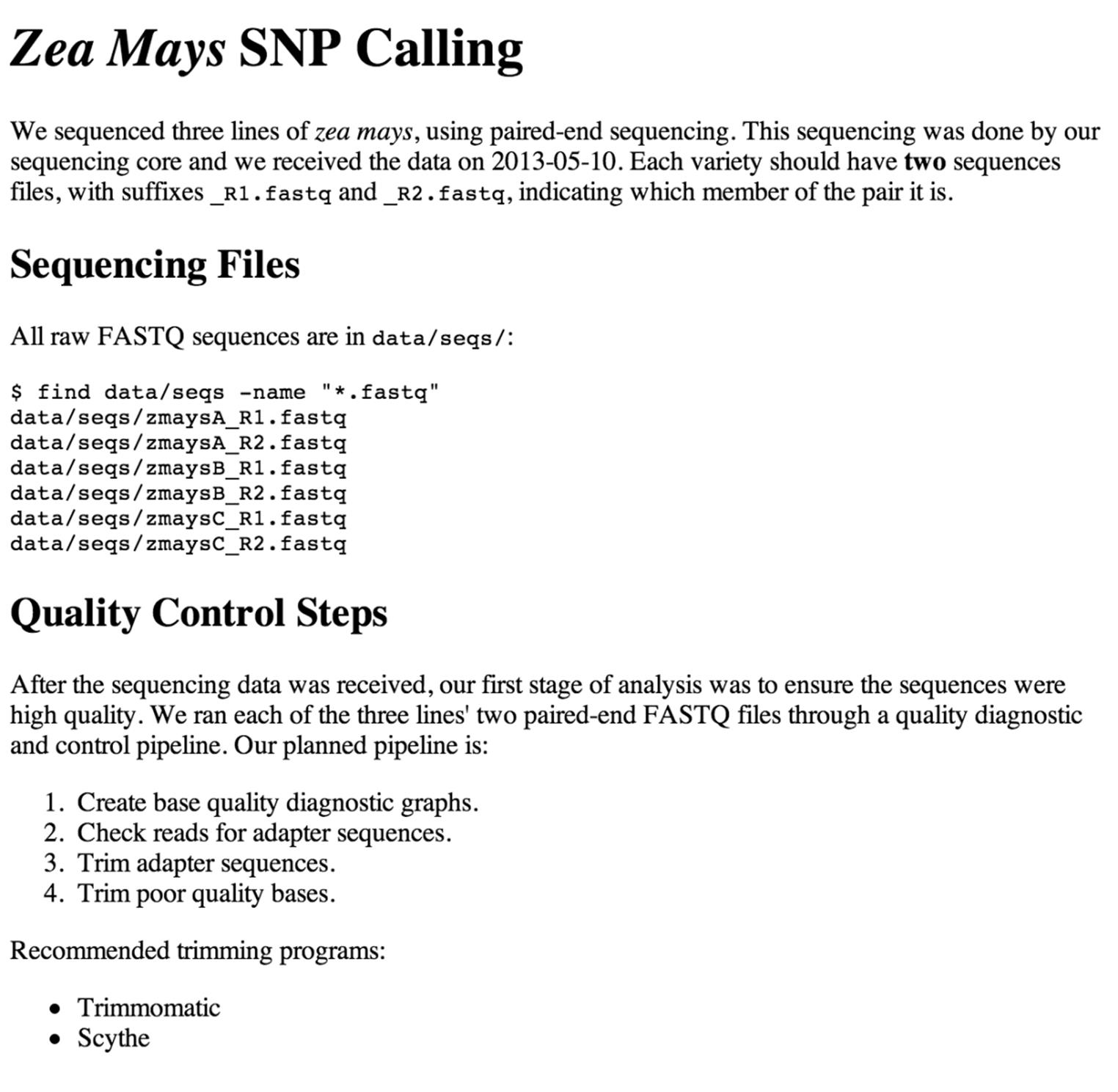
Figure 2-1. HTML Rendering of the Markdown notebook

Block elements like headers, lists, and code blocks are simple. Headers of different levels can be specified with varying numbers of hashes (#). For example:

# Header level 1

## Header level 2

### Header level 3

Markdown supports headers up to six levels deep. It’s also possible to use an alternative syntax for headers up to two levels:

Header level 1

==============

Header level 2

--------------

Both ordered and unordered lists are easy too. For unordered lists, use dashes, asterisks, or pluses as list element markers. For example, using dashes:

- Francis Crick

- James D. Watson

- Rosalind Franklin

To order your list, simply use numbers (i.e., 1., 2., 3., etc.). The ordering doesn’t matter, as HTML will increment these automatically for you. However, it’s still a good idea to clearly number your bullet points so the plain-text version is readable.

Code blocks are simple too — simply add four spaces or one tab before each code line:

I ran the following command:

$ find seqs/ -name "*.fastq"

If you’re placing a code block within a list item, make this eight spaces, or two tabs:

1. I searched for all FASTQ files using:

find seqs/ -name "*.fastq"

2. And finally, VCF files with:

find vcf/ -name "*.vcf"

What we’ve covered here should be more than enough to get you started digitally documenting your bioinformatics work. Additionally, there are extensions to Markdown, such as MultiMarkdown and GitHub Flavored Markdown. These variations add features (e.g., MultiMarkdown adds tables, footnotes, LaTeX math support, etc.) and change some of the default rendering options. There are also many specialized Markdown editing applications if you prefer a GUI-based editor (see this chapter’s README on GitHub for some suggestions).

Using Pandoc to Render Markdown to HTML

We’ll use Pandoc, a popular document converter, to render our Markdown documents to valid HTML. These HTML files can then be shared with collaborators or hosted on a website. See the Pandoc installation page for instructions on how to install Pandoc on your system.

Pandoc can convert between a variety of different markup and output formats. Using Pandoc is very simple — to convert from Markdown to HTML, use the --from markdown and --to html options and supply your input file as the last argument:

$ pandoc --from markdown --to html notebook.md > output.html

By default, Pandoc writes output to standard out, which we can redirect to a file (we’ll learn more about standard out and redirection in Chapter 3). We could also specify the output file using --output output.html. Finally, note that Pandoc can convert between many formats, not just Markdown to HTML. I’ve included some more examples of this in this chapter’s README on GitHub, including how to convert from HTML to PDF.