Better Business Decisions from Data: Statistical Analysis for Professional Success (2014)
Part V. Relationships
Chapter 16. Multivariate Data
Variety Is the Spice of Life
Practical problems often make it difficult to obtain homogeneous and similar samples. For example, samples may involve individuals of different ages and may have to be taken on different days of the week. Individuals differ in numerous ways, and real effects can arise on different days. It could be said, quite rightly, that samples differ because a variety of effects are always present, each creating a difference. In other words, no matter how we aim to obtain homogeneous samples, we will end up with multiple effects. In the past, when analysis involved lengthy procedures, this was a nuisance. Now, with the availability of computer packages that provide rapid and more versatile processing, multivariate data analysis is seen to be a great advantage and has in many areas taken over from the simplistic methods I have been describing.
The availability of rapid computer processing has brought with it other features. One is the increasing number of new methods that are appearing. New methods bring greater sophistication during processing but greater difficulty in understanding the detail involved, and controversy over their applicability to particular situations. An accompanying drawback to the ease of processing is that it becomes easy to search for any possible relationship that appears to be suggested by the data. As I have pointed out before, if enough correlations are sought, a number of spurious ones will be found, simply because of the probability governing the indication of significance. The relationships sought should be defined before the data is examined.
Chapter 4 mentioned the large databases that many organizations have. The data is potentially the source of unknown useful relationships; and sophisticated, computer-intensive procedures are used to extract those relationships. This process is referred to as data mining, and progress in developing and applying such methods has promoted data mining to an important subject in its own right. In a way, this compromises what I said above, that required possible relationships should be defined before the data is searched. The issue is discussed further in Part VII.
A drawback of computer processing is that the visibility of the processing is lost. The data is fed into the program, and the results are quickly displayed. In this chapter, it would be pointless to attempt to illustrate the processing of the data in detail. More useful to you will be a guide to the appropriateness of various methods, an outline of what each method does, and a guide to interpreting the results. Another drawback of computerized procedures is that anyone—even someone who lacks understanding of the methods, their restrictions, and their proper interpretation—can carry out analyses and produce conclusions.
The need for large samples has been mentioned a number of times. Here, because many different effects are involved, the samples need to be large in relation to each effect of interest. Note, though, that too large a sample may result in a large number of effects being found to be significant but with little practical use or meaning. In the sample, every feature is real. The larger the sample, the greater the number of variables that will be found to be significant. Ultimately, as the sample size approaches the total population, every feature of each datum becomes significant and reflects the fact that in the population, every feature is real.
You saw previously the difference between dependent and independent variables. A dependent variable is one that we observe rather than control, or the one we are attempting to predict. An independent variable is one that we fix or is fixed for us by circumstances. Thus, if we wish to see how illness varies with age, illness is the dependent variable and age is the independent variable. Clearly, illness depends on age, whereas age does not depend on illness. The distinction between the two kinds of variables is important in choosing the appropriate multivariate analysis method.
Previously we have separated numerical data from descriptive data in presenting the various techniques. The distinction becomes blurred when we are dealing with multivariate data. We may have both numerical and descriptive data involved in the same relationship. Also, we can in some methods render descriptive data numerical by the use of dummy variables. A dummy variable is a numerical code representing a descriptive variable. For example, if we have male or female as one of the variables, male could be coded as 0 and female as 1. With three levels of description, the coding could be 0, 1, and 2, and so on. The various methods described in the following sections are ordered generally from numerical to descriptive; but as you will see, there is considerable overlap.
Multiple Regression
If there is one dependent numerical variable and several independent numerical variables, multiple regression may be used. We may, for example, wish to know how much a person generally pays when buying a car, in relation to the person’s age, income, and savings. The principle is the same as in simple linear regression (Chapter 14). The squares of the differences between the observed values and the predicted values are minimized. In other words, the analysis is in terms of variance.
The form of the relationship used is
y = a + bx1 + cx2 + dx3 + … ,
where y is the dependent variable (i.e., the cost of the car in the example above), and x1, x2, x3, .... are the independent variables (age, income and savings, etc.). The letters a, b, c, d, .... represent constants, and the purpose of the analysis is to determine the best values for these constants. The form of the equation is linear—in other words, values of y plotted against one of the x values, the other x values being held constant, would yield a straight line.
However, this does not mean that curvature cannot be accommodated. If the data suggested that an increase in savings had an ever-increasing effect as the savings increased, we could add x32, i.e. the square of savings, in the linear equation. The equation would then be
y = a + bx1 + cx2 + dx3 + ex32
The data may suggest other non-linear relationships, and transformation of the variables can be used to modify the equation appropriately. For example, c(1/x2) might take the place of cx2 by transforming the x2 data values to 1/x2. The dependent variable, y, may also be transformed if necessary. The equation can also incorporate possible interactions between the variables. For example, we might decide to include a term f(x1x3 ) to allow for interaction between age and savings. In other words, we would be allowing for the likelihood that the influence of savings would be different for different age groups. It must be remembered that the fit of the regression equation is based on minimizing the errors of the transformed variables and not the original variables.
When the constants a, b, c, d, … have been calculated and the regression equation has been obtained, we need a measure of the usefulness of the equation. The multiple coefficient of determination, R2, is analogous to r2 that we met in relation to simple linear regression with two variables. R2indicates, in a similar manner, the proportion of the variation in y that is accounted for by the equation. The closer the value of R2 is to unity, the better the equation fits the data. Note, however, that although the equation may be useful, it may not be the best possible. It could be that a different selection of variables or a different transformation of variables would give a more useful equation.
Note also that as more variables are included the value of R2 will approach unity. Indeed when the number of variables equals the number of data then R2 = 1. There is also an increase in R2 as the sample size increases. An adjusted value of R2, the adjusted coefficient of determination, which compensates for the increase in sample size and number of variables, is usually quoted in the results provided by computer packages.
Unless the sample consists of the total population, it is necessary to establish the reliability of using the regression equation to represent the population. The variance ratio test, or F-test, described in Chapter 10, can be used to test at an appropriate significance level whether R2 differs from zero, in other words whether there is a significant relationship. Additionally, each of the constants in the regression equation, b, c, d, … , can be tested using Student’s t-test to establish whether it differs significantly from zero and at what level of significance. A constant found not to differ significantly from zero indicates that the associated variable can be removed without affecting the usefulness of the correlation.
Descriptive variables can be included in multiple regression analysis by the use of dummy variables, though the dependent variable must be numerical. A technique known as canonical correlation extends the principle of multiple regression to dealing with several numerical dependent variables and several numerical independent variables. With the use of dummy variables, the technique can be extended to dealing with several descriptive dependent variables and several descriptive independent variables.
Analysis of Variance
You saw in Chapter 10 how analysis of variance (ANOVA) can be used to compare two or more samples in order to decide whether they could have been drawn from the same population. The method can be extended to analyze data that is influenced by more than one effect. For example, suppose we have test results for students in four subjects. We wish to investigate whether there is a difference between the results for boys and girls and whether ability in different subjects is related. Here we have two effects, or factors—subject and gender—and both of these are descriptive. These are the independent variables, while the dependent variable, which is numerical, is the mark obtained in the test.
Thus the data might be as follow:
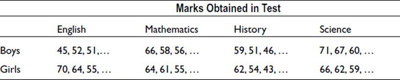
For this type of analysis, it is necessary to have a numerical dependent variable and several descriptive independent variables. The analysis of variance will allow the total variance in the data to be partitioned between the various sources of variance. In this example, there is a variance attributed to the gender of the students and a variance attributed to the test subject. In addition, there is variance due to interaction between these two main effects. Interaction arises when the effect of gender is different in relation to different subjects: boys may be better than girls in science but poorer than girls in English. There is also a contribution to the total variance from effects that are not included in the analysis. This is the residual variance.
To illustrate the method we will outline the working through of an example with three effects and a replication of the data.
A company has three factories, and in each factory are three slightly different machines, versions 1, 2, and 3. On most days, the machines suffer from overheating of up to 3 degrees. The company wishes to see if the overheating is related to the version of the machines or to the circumstances of use in the three factories. The operating temperature of each machine is observed, and the excess temperature is recorded. In case the day of the week is relevant, records are taken on five days from Monday to Friday. The exercise is repeated the following week to give a measure of replication. The results are assembled as follows:
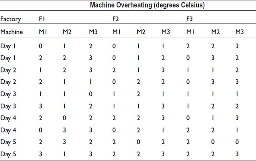
Note that the numbers here are all small integers. This is purely to keep the illustration simple. In a practical situation we would expect to have numbers consisting of several digits.
The ninety values listed have a variance which is due to a number of factors. The variability between factories, between machines, and between days of the week contributes to the overall variance. Interactions between each pair of variables and between all three variables may contribute. In addition, there are almost certainly other sources of variation that cannot be identified. The analysis of variance allows the total variance to be apportioned between the various factors. It is this additive property of variances that makes the analysis of variance such a powerful tool.
It would not be helpful to plow through the arithmetic in detail: computer packages are available to do the job. More useful is an explanation of what the calculation does.
The first three columns of the above table are the results from factory F1, thirty in total. If we were to temporarily replace each value with the mean value of the thirty, and do the same for F2 and F3, we would have a set of ninety values, the variance of which would reflect the variation due to any differences between the factories. Similarly, we can obtain three sets of adjusted values reflecting the variation due to machines and five sets of adjusted values reflecting the variation due to the different days of the week. Note that the degrees of freedom associated with the variances are reduced by this substitution of mean values. The variance of F has only two degrees of freedom because only three mean values are being used, despite the fact that there are ninety data.
The breakdown of the overall variance can be taken further. There are 9 sets of data which include the variation due to factories and machines. These are the 9 columns in the table. By again substituting the set mean value for each value in the set, a variance can be calculated. By removing the already obtained separate effects of factory and machine, we are left with a variance relating to interaction between factory and machine. That is to say, the behavior of the corresponding machine depends to some extent on which factory it is located in.
There are 15 sets of data that include the variation due to machines and days, and 15 sets of data that include the variation due to days and factories. There are 45 sets of data, albeit only 2 values in each set, that include the variation due to factories, machines, and days; and, finally, there is the complete set of 90 values that additionally includes variation due to other factors and random effects. Each set of values can in turn be temporarily modified by substituting the mean of the set for each member value, and the variance can be adjusted by removing the single factor effects, leaving the variance attributable to the interaction.
I must add that this is not the way one would actually carry out the calculations—as you would probably use a computer package—but it is a way of seeing what in effect is being done.
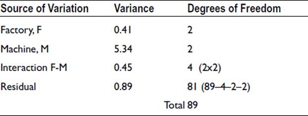
The results of all this can be laid out as follow:
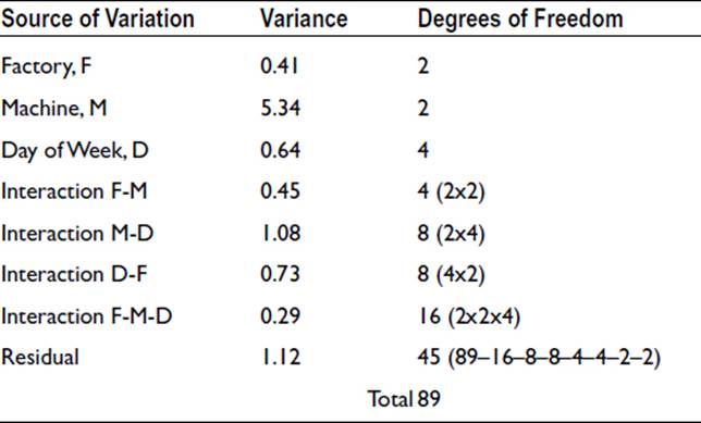
The residual variance is a measure of the variation that would be observed in the absence of any effect arising from the particular factory, particular machine, or particular day of the week. In other words, random or unknown effects are producing a variance of this size. We can therefore test whether any of the other variances are significantly greater than the residual variance. The test to use is the variance ratio test, F-test. In the above example, only one variance is greater than the residual variance: the variance due to machine. So, this is the only one that needs testing. The variance ratio is 5.34/1.12 = 4.77, which is found to be significant at the 5% level. A relevant extract from the tables of the F-statistic is shown as follows:
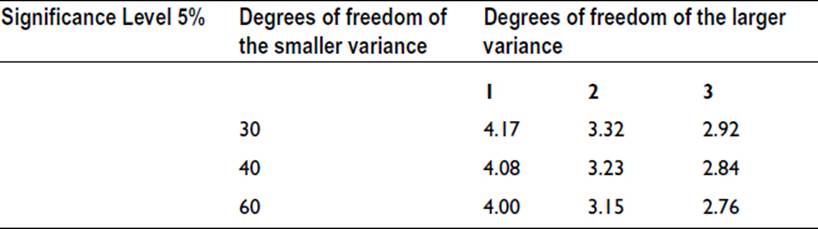
Thus we can conclude that the variation between machines is likely to be a real effect. We can also conclude that there is no significant evidence that overheating is more prone in one factory than another, nor that overheating is related to the day of the week.
Two additional points need to be mentioned regarding interactions. First, if an interaction is found to be significant, then the main factors in the interaction cannot be tested. The situation has to be investigated further. Second, if the interactions are not significant, then their variances are an additional measure of the residual variance. They can therefore be pooled with the residual variance.
By pooling some of the variances that are not significant, we can gain further appreciation of the versatile nature of the analysis of variance. Pooling the D, M-D, D-F, F-M-D, and residual variances gives a value of 0.89 for the revised residual variance. The results now appear as follow:
The point of interest here is that if we had, at the outset, decided that the day of the week was unlikely to have any effect on the results, we could have treated the values obtained on different days as replicates. Thus we would have had 9 combinations of factory and machine and 10 data for each combination. The analysis would have been in terms of two main effects, F and M, and one interaction, F–M. The results would have come out exactly as shown above with a residual variance of 0.89.
It is useful to show the results of the machine overheating example by plotting a number of graphs. The significant effect of machine type can be seen in Figure 16-1, where the mean overheating temperature for each machine is plotted against the machine number. Similar graphs for the two non-significant main effects are also shown. There is no reason why these graphs should have a particular shape: any appreciable departure from a horizontal line might indicate a significant effect.
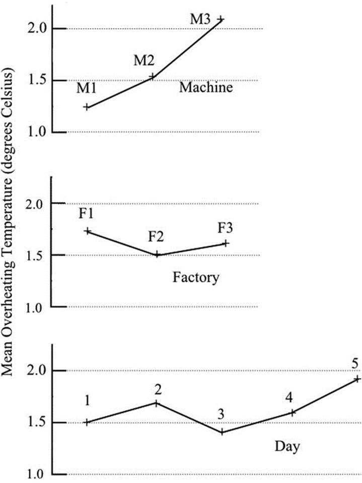
Figure 16-1. Comparison of overheating of different machines in different factories on different days
Latin and Graeco-Latin Squares
A version of analysis of variance uses Latin or Graeco-Latin squares, typically in agricultural experiments. If fertilizers are to be compared in terms of crop yield, for example, there is always the possibility that the fertility of the land used for the study may vary from place to place. Clearly, it is not possible to test all the fertilizers in the same place at the same time: each one is tested where the fertility may be different.
In the Latin square arrangement, the rectangular test area is divided into smaller plots, forming a grid of rows and columns. Each fertilizer is used once in each row and once in each column. Thus if we have four different fertilizers designated A, B, C, and D, the arrangement could be as follows:
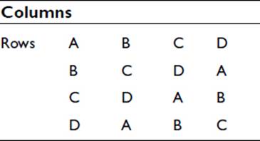
This corresponds to 16 data of the crop yield, 4 for each of the treatments A, B, C, and D. The crop yield is the dependent variable, and the fertilizer brand and soil fertility are the independent variables. The analysis of variance can be arranged as follows:
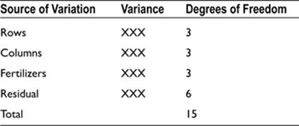
The rows and columns variances reflect the variability in the soil characteristics across and down the experimental area. Note that there are no variances listed for interactions. This is a consequence of the Latin square design. Only one fertilizer is applied to a plot of a given fertility, giving a considerable saving in the number of plots required. The actual number of combinations of fertilizer and soil fertility is 4 x16 = 64. The use of 64 plots would not be feasible: apart from the larger test area required and the extra cost, there would be additional variation in soil fertility because of the increased test area.
An additional effect can be included by the use of a Graeco-Latin square as shown below. The Latin letters A to D represent four treatments, as before, and the Greek letters α to δ represent a second treatment—pesticide, say:
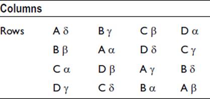
As in the Latin square, each fertilizer is used only once in each row and column. Furthermore, each pesticide is used only once with each fertilizer. Squares of different sizes can be set up, but the arrangement is not possible for a square of side 6.
Although the description has been in terms of agricultural experiments, because that is where the practical applications have mainly been, the squares can be used elsewhere. They are particularly useful when it is essential, for reasons of cost, time, or accessibility, to keep the number of observations to a minimum.
Medical studies often fall into this category. If it were required to investigate four different treatments for an ailment, four suitable patients could be selected. Suppose it takes one month to assess the effects of each treatment. The columns in the Latin square shown above would be the four treatments, and the rows would be four consecutive months. The letters A, B, C, and D would represent the four patients. At the end of one month, all four treatments would have been tested; and after four months, there would be 16 sets of data representing the outcome of each treatment administered to each patient.
It can be seen from this medical example that the Latin square can be a very efficient means of investigation, particularly when interactions between the main effects are not considered likely. If there were to be appreciable interactions, the effect would be to increase the residual variance and make it more difficult to verify any significant difference between the treatments.
The Latin square can be modified by removing a row or a column. The resulting rectangular arrangement is known as a Youden square.
TIRE TRIALS
As chief accountant for ZIP Deliveries, Mark Groves was always looking for ways to cut back on expenditure. The company ran a parcel delivery service and had a fleet of about forty vans. The field was very competitive and costs were important.
Tires for the vehicles cost an appreciable amount, and that was what Mark was currently considering. At present the company was purchasing a cheap brand of tire, but perhaps it would pay to use a more expensive brand and achieve a longer life.
Three other brands were readily available, and Mark proposed an experiment to compare them with the brand currently being used. He had in mind a Latin square arrangement. Four vans would be fitted with new tires, each van with a different brand. The four vans, each with its regular driver, would constitute the columns of a 4 × 4 Latin square. Four daily routes, each of similar distance but, of course, different road conditions, would constitute the rows of the square.
For the experiment, each van would spend a month working each of the designated routes. The tire wear would be recorded by measurements of tread depth carried out by the garage maintenance team.
The Latin square arrangement ensured that the effect of the four different drivers and the effect of the four different routes would be separated from the effect of the different brands of tire.
Having got approval for the experiment, Mark took a standard 4 × 4 Latin square, put the columns in a random order, put the rows in a random order, and allocated the four brands to the lettered squares A, B, C, and D. This provided the schedule for the routes for the four vans, and the trial went ahead.
At the end of the trial period, Mark analyzed the results. He found that the variance due to the vans was not significant. The variance due to the routes was significant at the 5% level, which was perhaps not too surprising. Importantly, the variance due to the tire brands was significant, well inside the 5% level. Thus the difference between the different brands could be accepted as being real.
For each of the brands, Mark used the tire-wear values and the cost to calculate which brand would be most cost effective. It turned out to be one of the more expensive ones, so the exercise had not been a waste of time, much to Mark's relief. It was decided that the tire contract would be changed accordingly, and Mark had a smile on his face for the rest of the day.
Multidimensional Contingency Tables
You saw in Chapter 15 how the association between two descriptive variables can be compared by means of a contingency table. If we have more than two variables, we have in effect a table with three or more dimensions. Such tables can, of course, be laid out as several two-dimensional tables; but in order to explain how to proceed, it is useful to emphasize the multidimensional nature of the situation by attempting to give a perspective view of a three-dimensional one. This has been done in Figure 16-2.
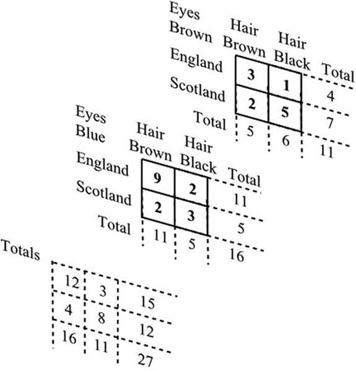
Figure 16-2. A three-way contingency table
The three independent variables are place of birth, color of hair, and color of eyes, and the dependent variable is the number of cases. The task is again to replace the actual sampled values temporarily with expected values based on the assumption that there is no significant effect from the variables. The values, in other words, are not significantly different from values that would be obtained from the overall proportions of each category. However, unlike the situation where we had only two variables, there is not a unique expected value. Judgment is needed to fix the best expected value.
To see where the problem lies, consider the table for blue eyes extracted from Figure 16-2. The expected values are as follow:
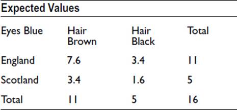
For example, 7.6/11 = 3.4/5 = 11/16.
If we now look down from above on our three-dimensional table, the top layer appears as follows:
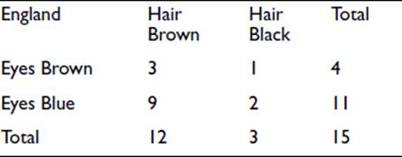
And if we calculate the expected values, we get the following:
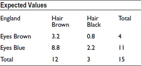
For example, 3.2/12 = 0.8/3 = 4/15.
Our expected value for England – Hair Brown – Eyes Blue is now 8.8, whereas our first calculation of expected values gave 7.6. The reason, of course, is that the first value is expected if Brown Eyes are excluded, and the second value is expected if Scotland is excluded. The same problem arises for each of the eight combinations of place of birth, hair color, and eye color.
The analysis that is used in these situations to overcome the problem is called log-linear. It is a lengthy iterative procedure that makes repeated estimates of the expected values and is thus computer intensive. The “log” in the title refers to the fact that the logarithms of the values are used to give additive properties in the processing. The technique is analogous to the analysis of variance shown earlier for dealing with numerical data when several variables are involved. There you saw that not only was there a main effect from each variable but we had interactions from each pair of variables, each triplet of variables, and so on. You also saw that the use of variance allowed us to partition the variability between the main effects and the interactions.
We have a similar situation here with our multidimensional contingency tables. Interaction here means, for example, that the effect of place of birth and hair color on color of eyes, acting together, is not the same as the sum of the effects acting separately. The processing involves an element of judgment. An approach from the top down would estimate the optimum expected values on the basis of three main effects. If the residual variability were too great, as indicated by its level of significance, the second-order interactions would be included, and so on. In the example, the third-order interaction involving all three variables cannot be dealt with, because the values as they were sampled may be the expected values. If we had a duplicate sample, the third-order interaction could be isolated from the residual variation. The example given in the “Analysis of Variance” section involved a duplicate sample and allowed this separation.
An alternative direction of processing is from the bottom up. Starting with the inclusion of all main effects and interactions, the significance of the highest-order interactions is checked. If not significant these interactions are removed from the activity of estimating the expected values. This continues until the only effects remaining are those with an acceptable level of significance.
A variation of log-linear analysis is logit analysis. This allows the use of a dependent variable that is not numerical but can take one of two descriptive labels: male or female, for example. The proportion of males (or females) is restricted to values between 0 and 1. The logit, or log odds, function transforms the proportion to a value having an unlimited range from minus infinity to plus infinity.
Multivariate Analysis of Variance
An extension of the analysis of variance (ANOVA) is the multivariate analysis of variance (MANOVA). You saw that the analysis of variance was able to deal with multiple effects but only when we had a single dependent variable and several independent variables. In multivariate analysis of variance, we are able to deal with several dependent variables.
As an example, suppose the bakery departments of two supermarkets are to be compared. Three different products are involved: loaves, buns, and cakes. The two dependent numerical variables on which the comparison will be based are profit and customer satisfaction. The variables are thus as follow:
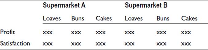
For each level of each variable there will be a data sample, represented by xxx above. As the number of data groups increases, the need for large sample sizes increases. Each group must have a size greater than the number of variables and should have not fewer than about 20 data.
In the analysis of variance, partitioning of the variance produces values of the variance ratio, F, which can be used to evaluate the effect of each independent variable on the dependent variable. In multivariate analysis, we use a corresponding statistic to evaluate each effect on each dependent variable. There are a number of possible statistics: Wilks’s lambda, the Hotelling-Lawley trace, the Pillai-Bartlett trace, and Roy’s maximum root. The effect of interactions is examined first, as in the analysis of variance. If an interaction is found to be not significant, the constituent variables can each be tested for significance.
The processing is complicated and may involve additional routines to ensure reliability of the results: hence the need for a suitable computer package. Underlying statistical assumptions regarding the data also may have to be examined. The interpretation of the results needs considerable care. Because there are potentially many effects to be identified, the power of the test—that is, the ability to detect a relationship when it exists—may be low. In order to ensure that the power is sufficiently large to identify small effects, the required sample size may be prohibitively large.
Conjoint Analysis
Conjoint analysis is used to investigate customer evaluations of products or services. It differs from other techniques in that the investigator sets up at the outset combinations of features representing real or hypothetical versions of the product. These are the independent variables. Thus the sampled consumers merely rank the combinations rather than create variables by the nature of their replies. For example, a deodorant could be produced in the form of a roll-on, a pump spray, or an aerosol, each in one of three colors of container, and each in one of two sizes. This would give a total of 18 possible combinations. The three independent variables—form, color, and size—are descriptive, and the dependent variable is the preference of each combination as recorded by its rank order.
From the rankings supplied by each sampled consumer, the part-worth of each factor can be evaluated, taking account of interaction effects. It is not necessary to present each respondent with all combinations: a selection can be used to provide data for evaluation. A feature not present in most other methods is that an evaluation can be obtained for a single respondent. Results from several respondents can be aggregated to provide an overall assessment of the separate attributes of the product or potential product.
Proximity Maps
Association between descriptive variables can be visually presented by means of a map on which the degree of association between two items is represented by the distance between them. Greater degrees of association are indicated by closer spacing. Two- or three-dimensional maps can be shown as diagrams, of course, but if more than three dimensions are involved, only “slices” of the map can be visually appreciated.
Correspondence analysis is one such method. The data is represented in a contingency table, as discussed in Chapter 15 and the “Multidimensional Contingency Tables” section of this chapter. The analysis follows the procedure we described for multiway contingency tables in obtaining an expected value for each cell on the basis of no association. The difference between each actual and expected value is expressed as a value of the chi-squared statistic, which provides a measure of association. Distances for mapping are then computed in relation to the chi-squared values: the larger the value, the smaller the distance.
To illustrate the method in a simple manner, we can use the two-way contingency table from Chapter 15 that related color of hair to place of birth. The table is repeated here:

The expected numbers, on the basis of there being no association, were calculated as follows:
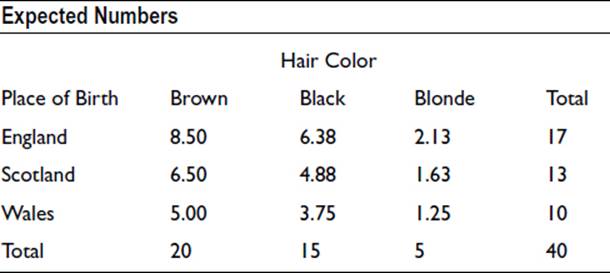
The statistic chi-squared is equal to the square of the difference between the expected and observed values, divided by the expected value. It is calculated for each cell in the table as shown below. (Negative values, when the observed is less than the expected, are treated as positive in calculating the chi-squared totals.)
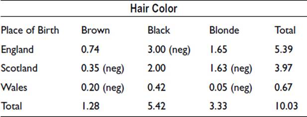
These values provide a measure of similarity for each pair of variable levels, the largest values representing the largest positive association. Negative values represent negative association. (It may be noted that the sum of the above chi-squared values, 10.03, was used in Chapter 15 to show that there was a significant relationship between hair color and place of birth.)
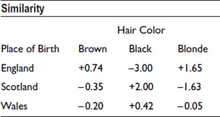
We can use the similarity values to produce a map. Each of the nine values provides a distance that is used to separate the pair of variable levels: the larger the value, the smaller the distance. Figure 16-3 illustrates an approximate arrangement. Scotland-Black has the top position in ranking and the smallest separation, whereas England-Black has the bottom position and the largest separation. The map shows various degrees of association. Brown and blonde hair are closely associated with English individuals, whereas black hair is associated more so with Welsh and Scottish people. You will appreciate that the separations cannot be exactly as required: there has to be compromise to fit the variables together. In a practical application, a computer package would apply an iterative procedure to optimize the fit.
Figure 16-3. A map showing association between hair color and place of birth
The maximum number of dimensions that can be used is one less than the fewest number of levels for either variable: in this case, two. A realistic study might have more variables, each with more levels, and hence a map with a greater number of dimensions. To obtain the optimum set of distances that provides a consistent arrangement then requires a lengthy iterative procedure and is feasible only with the aid of a computer program.
Multidimensional scaling is similar to correspondence analysis in employing a multidimensional map to reveal association. It differs in that the variables are not defined at the outset; it is more a case of establishing the underlying variables from the analysis of the sample data. The technique represents perceived similarities or preferences between entities as the distances between them on a map. For example, six kinds of breakfast cereal could be compared two at a time by each volunteer in order to provide a sample. The comparison could be on a scale of 1 to 10, say. Six items produces 15 pairs for comparison; and to map the items in a consistent manner, with regard to correct relative separations, several dimensions are likely to be required for the map. Procedures for optimizing the mapping positions while minimizing the number of dimensions require judgment and repeated calculations.
The resulting map dimensions provide information as to the underlying features that prompt the recorded perceptions. It may be that degree of sweetness appears to lie along one dimension while “crunchiness” lies along another. It will be appreciated that considerable judgment is required in the interpretation. A feature of the method is that each respondent provides a sample which can be individually analyzed. Individual analyses can, of course, be aggregated.
Structural Equation Modeling
In the methods for dealing with multiple effects that have been discussed so far there has always been the limitation that there has been a single relationship between the dependent and the independent variables. It is sometimes the case that several interrelated relationships need to be established simultaneously. Structural equation modeling can be used when confirmation of a theory of such relationships is sought, but it is not useful at the exploratory stage.
A model based on theoretical judgments is set up, consisting of a number of variables linked by (assumed) causal relationships. Thus if we are concerned with the reputation of a school, for example, we may propose that success in examinations (a) depends on student ability (b) and teaching quality (c). Teaching quality depends on quality of teachers employed (d) and available resources (e). Quality of teachers employed depends on success in examinations and location (f). Student ability depends on available resources and location. In symbols, we have
a = w1b + w2c
c = w3d + w4e
d = w5a + w6f
b = w7e + w8f
where w1 … w8 are weights to account for different degrees of influence. In effect, we have something similar to a set of multiple regression equations that are interrelated.
The processing is complex and not unique. It involves path analysis and is related to factor analysis and regression. The method has the ability to encompass latent variables that are not directly measured but that emerge from the measured variables. To achieve satisfactory results requires much care in setting up the initial model, establishing an acceptable goodness of fit, and interpreting and modifying the model.
Association: Some Further Methods
Some practical situations, like the example in the previous section concerning the reputation of a school, involve variables that are not only descriptive but subjective and difficult to define precisely. The levels adopted by the variables may also be subjective and difficult to define. Furthermore, there may be many such variables of interest. Such situations arise in marketing and product development. Hair brushes may vary in size, shape, color, shape of handle, feel of handle, and so on. Customer evaluation of the brushes may involve comfort in use, effectiveness in brushing, aesthetic appeal, and more. In sociology or psychology studies, attitudes and opinions can range between extremes with no clear means of scaling the in-between values. Degrees of friendliness, luck, ambition, pain, happiness, and so forth are difficult to scale.
Methods are available that can assist in reducing variables and their levels by identifying significant similarities. Many of these are interdependence methods in that there is no distinction between dependent and independent variables. The mathematics involved is usually complicated and requires considerable background knowledge. Furthermore, the planning of appropriate procedures and the interpretation of the results needs care.
Factor analysis is a method of analyzing relationships among a large number of variables in order to represent the data in terms of a smaller number of factors. All the variables are treated on an equal footing: there is no distinction between dependent and independent variables. As an example, we might consider customers’ assessments of a dental practice under a variety of headings such as ease of booking an appointment (a), availability of suitable time slots (b), time spent in the waiting room (c), friendliness of staff (d), efficiency of staff (e), quality of treatment (f), and so on. Each assessment would be numerical, on a scale of 1 to 10, say. The correlation between each pair of variables would be determined, the six variables listed giving rise to 15 correlations. From these, an optimum grouping of the variables would be found, minimizing the variance within the groups and maximizing the variance between groups. It might be established, for example, that three groups—(a)-(b)-(c), (d)-(e) and (f) in the example above—adequately provide the required assessment. A similar method is principal components analysis.
Cluster analysis is similar to factor analysis but is used to group entities, rather than variables. The entities resemble each other in showing similar attributes. The characteristics of the clusters are not defined at the outset but arise in the process. People might be grouped according to their personal features or characteristics. The process is equally applicable to all kinds of things, such as cars, birds, or hats, for example.
In multiple discriminant analysis, groups are defined, and the process locates items in the appropriate group while maximizing the probability of correct location. The technique deals with a single descriptive dependent variable and several numerical independent variables. For example, the technique might be used to separate potential customers from unlikely customers based on several numerically designated characteristics.
This brief overview of methods for dealing with multivariate data is by no means exhaustive. The availability of computers that can perform iterative procedures at incredibly high speeds has given statisticians the means of employing and developing methods with greater and greater sophistication.
All materials on the site are licensed Creative Commons Attribution-Sharealike 3.0 Unported CC BY-SA 3.0 & GNU Free Documentation License (GFDL)
If you are the copyright holder of any material contained on our site and intend to remove it, please contact our site administrator for approval.
© 2016-2026 All site design rights belong to S.Y.A.