Elasticsearch: The Definitive Guide (2015)
Part IV. Aggregations
Chapter 34. Controlling Memory Use and Latency
Fielddata
Aggregations work via a data structure known as fielddata (briefly introduced in “Fielddata”). Fielddata is often the largest consumer of memory in an Elasticsearch cluster, so it is important to understand how it works.
TIP
Fielddata can be loaded on the fly into memory, or built at index time and stored on disk. Later, we will talk about on-disk fielddata in “Doc Values”. For now we will focus on in-memory fielddata, as it is currently the default mode of operation in Elasticsearch. This may well change in a future version.
Fielddata exists because inverted indices are efficient only for certain operations. The inverted index excels at finding documents that contain a term. It does not perform well in the opposite direction: determining which terms exist in a single document. Aggregations need this secondary access pattern.
Consider the following inverted index:
Term Doc_1 Doc_2 Doc_3
------------------------------------
brown | X | X |
dog | X | | X
dogs | | X | X
fox | X | | X
foxes | | X |
in | | X |
jumped | X | | X
lazy | X | X |
leap | | X |
over | X | X | X
quick | X | X | X
summer | | X |
the | X | | X
------------------------------------
If we want to compile a complete list of terms in any document that mentions brown, we might build a query like so:
GET /my_index/_search
{
"query" : {
"match" : {
"body" : "brown"
}
},
"aggs" : {
"popular_terms": {
"terms" : {
"field" : "body"
}
}
}
}
The query portion is easy and efficient. The inverted index is sorted by terms, so first we find brown in the terms list, and then scan across all the columns to see which documents contain brown. We can very quickly see that Doc_1 and Doc_2 contain the token brown.
Then, for the aggregation portion, we need to find all the unique terms in Doc_1 and Doc_2. Trying to do this with the inverted index would be a very expensive process: we would have to iterate over every term in the index and collect tokens from Doc_1 and Doc_2 columns. This would be slow and scale poorly: as the number of terms and documents grows, so would the execution time.
Fielddata addresses this problem by inverting the relationship. While the inverted index maps terms to the documents containing the term, fielddata maps documents to the terms contained by the document:
Doc Terms
-----------------------------------------------------------------
Doc_1 | brown, dog, fox, jumped, lazy, over, quick, the
Doc_2 | brown, dogs, foxes, in, lazy, leap, over, quick, summer
Doc_3 | dog, dogs, fox, jumped, over, quick, the
-----------------------------------------------------------------
Once the data has been uninverted, it is trivial to collect the unique tokens from Doc_1 and Doc_2. Go to the rows for each document, collect all the terms, and take the union of the two sets.
TIP
The fielddata cache is per segment. In other words, when a new segment becomes visible to search, the fielddata cached from old segments remains valid. Only the data for the new segment needs to be loaded into memory.
Thus, search and aggregations are closely intertwined. Search finds documents by using the inverted index. Aggregations collect and aggregate values from fielddata, which is itself generated from the inverted index.
The rest of this chapter covers various functionality that either decreases fielddata’s memory footprint or increases execution speed.
NOTE
Fielddata is not just used for aggregations. It is required for any operation that needs to look up the value contained in a specific document. Besides aggregations, this includes sorting, scripts that access field values, parent-child relationships (see Chapter 42), and certain types of queries or filters, such as the geo_distance filter.
Aggregations and Analysis
Some aggregations, such as the terms bucket, operate on string fields. And string fields may be either analyzed or not_analyzed, which begs the question: how does analysis affect aggregations?
The answer is “a lot,” but it is best shown through an example. First, index some documents representing various states in the US:
POST /agg_analysis/data/_bulk
{ "index": {}}
{ "state" : "New York" }
{ "index": {}}
{ "state" : "New Jersey" }
{ "index": {}}
{ "state" : "New Mexico" }
{ "index": {}}
{ "state" : "New York" }
{ "index": {}}
{ "state" : "New York" }
We want to build a list of unique states in our dataset, complete with counts. Simple—let’s use a terms bucket:
GET /agg_analysis/data/_search?search_type=count
{
"aggs" : {
"states" : {
"terms" : {
"field" : "state"
}
}
}
}
This gives us these results:
{
...
"aggregations": {
"states": {
"buckets": [
{
"key": "new",
"doc_count": 5
},
{
"key": "york",
"doc_count": 3
},
{
"key": "jersey",
"doc_count": 1
},
{
"key": "mexico",
"doc_count": 1
}
]
}
}
}
Oh dear, that’s not at all what we want! Instead of counting states, the aggregation is counting individual words. The underlying reason is simple: aggregations are built from the inverted index, and the inverted index is post-analysis.
When we added those documents to Elasticsearch, the string "New York" was analyzed/tokenized into ["new", "york"]. These individual tokens were then used to populate fielddata, and ultimately we see counts for new instead of New York.
This is obviously not the behavior that we wanted, but luckily it is easily corrected.
We need to define a multifield for state and set it to not_analyzed. This will prevent New York from being analyzed, which means it will stay a single token in the aggregation. Let’s try the whole process over, but this time specify a raw multifield:
DELETE /agg_analysis/
PUT /agg_analysis
{
"mappings": {
"data": {
"properties": {
"state" : {
"type": "string",
"fields": {
"raw" : {
"type": "string",
"index": "not_analyzed"![]()
}
}
}
}
}
}
}
POST /agg_analysis/data/_bulk
{ "index": {}}
{ "state" : "New York" }
{ "index": {}}
{ "state" : "New Jersey" }
{ "index": {}}
{ "state" : "New Mexico" }
{ "index": {}}
{ "state" : "New York" }
{ "index": {}}
{ "state" : "New York" }
GET /agg_analysis/data/_search?search_type=count
{
"aggs" : {
"states" : {
"terms" : {
"field" : "state.raw" ![]()
}
}
}
}
![]()
This time we explicitly map the state field and include a not_analyzed sub-field.
![]()
The aggregation is run on state.raw instead of state.
Now when we run our aggregation, we get results that make sense:
{
...
"aggregations": {
"states": {
"buckets": [
{
"key": "New York",
"doc_count": 3
},
{
"key": "New Jersey",
"doc_count": 1
},
{
"key": "New Mexico",
"doc_count": 1
}
]
}
}
}
In practice, this kind of problem is easy to spot. Your aggregations will simply return strange buckets, and you’ll remember the analysis issue. It is a generalization, but there are not many instances where you want to use an analyzed field in an aggregation. When in doubt, add a multifield so you have the option for both.
High-Cardinality Memory Implications
There is another reason to avoid aggregating analyzed fields: high-cardinality fields consume a large amount of memory when loaded into fielddata. The analysis process often (although not always) generates a large number of tokens, many of which are unique. This increases the overall cardinality of the field and contributes to more memory pressure.
Some types of analysis are extremely unfriendly with regards to memory. Consider an n-gram analysis process. The term New York might be n-grammed into the following tokens:
§ ne
§ ew
§ w
§ y
§ yo
§ or
§ rk
You can imagine how the n-gramming process creates a huge number of unique tokens, especially when analyzing paragraphs of text. When these are loaded into memory, you can easily exhaust your heap space.
So, before aggregating across fields, take a second to verify that the fields are not_analyzed. And if you want to aggregate analyzed fields, ensure that the analysis process is not creating an obscene number of tokens.
TIP
At the end of the day, it doesn’t matter whether a field is analyzed or not_analyzed. The more unique values in a field—the higher the cardinality of the field—the more memory that is required. This is especially true for string fields, where every unique string must be held in memory—longer strings use more memory.
Limiting Memory Usage
In order for aggregations (or any operation that requires access to field values) to be fast, access to fielddata must be fast, which is why it is loaded into memory. But loading too much data into memory will cause slow garbage collections as the JVM tries to find extra space in the heap, or possibly even an OutOfMemory exception.
It may surprise you to find that Elasticsearch does not load into fielddata just the values for the documents that match your query. It loads the values for all documents in your index, even documents with a different _type!
The logic is: if you need access to documents X, Y, and Z for this query, you will probably need access to other documents in the next query. It is cheaper to load all values once, and to keep them in memory, than to have to scan the inverted index on every request.
The JVM heap is a limited resource that should be used wisely. A number of mechanisms exist to limit the impact of fielddata on heap usage. These limits are important because abuse of the heap will cause node instability (thanks to slow garbage collections) or even node death (with an OutOfMemory exception).
CHOOSING A HEAP SIZE
There are two rules to apply when setting the Elasticsearch heap size, with the $ES_HEAP_SIZE environment variable:
No more than 50% of available RAM
Lucene makes good use of the filesystem caches, which are managed by the kernel. Without enough filesystem cache space, performance will suffer.
No more than 32 GB: If the heap is less than 32 GB, the JVM can use compressed pointers, which saves a lot of memory: 4 bytes per pointer instead of 8 bytes.
+ Increasing the heap from 32 GB to 34 GB would mean that you have much less memory available, because all pointers are taking double the space. Also, with bigger heaps, garbage collection becomes more costly and can result in node instability.
This limit has a direct impact on the amount of memory that can be devoted to fielddata.
Fielddata Size
The indices.fielddata.cache.size controls how much heap space is allocated to fielddata. When you run a query that requires access to new field values, it will load the values into memory and then try to add them to fielddata. If the resulting fielddata size would exceed the specified size, other values would be evicted in order to make space.
By default, this setting is unbounded—Elasticsearch will never evict data from fielddata.
This default was chosen deliberately: fielddata is not a transient cache. It is an in-memory data structure that must be accessible for fast execution, and it is expensive to build. If you have to reload data for every request, performance is going to be awful.
A bounded size forces the data structure to evict data. We will look at when to set this value, but first a warning:
WARNING
This setting is a safeguard, not a solution for insufficient memory.
If you don’t have enough memory to keep your fielddata resident in memory, Elasticsearch will constantly have to reload data from disk, and evict other data to make space. Evictions cause heavy disk I/O and generate a large amount of garbage in memory, which must be garbage collected later on.
Imagine that you are indexing logs, using a new index every day. Normally you are interested in data from only the last day or two. Although you keep older indices around, you seldom need to query them. However, with the default settings, the fielddata from the old indices is never evicted! fielddata will just keep on growing until you trip the fielddata circuit breaker (see “Circuit Breaker”), which will prevent you from loading any more fielddata.
At that point, you’re stuck. While you can still run queries that access fielddata from the old indices, you can’t load any new values. Instead, we should evict old values to make space for the new values.
To prevent this scenario, place an upper limit on the fielddata by adding this setting to the config/elasticsearch.yml file:
indices.fielddata.cache.size: 40% ![]()
![]()
Can be set to a percentage of the heap size, or a concrete value like 5gb
With this setting in place, the least recently used fielddata will be evicted to make space for newly loaded data.
WARNING
There is another setting that you may see online: indices.fielddata.cache.expire.
We beg that you never use this setting! It will likely be deprecated in the future.
This setting tells Elasticsearch to evict values from fielddata if they are older than expire, whether the values are being used or not.
This is terrible for performance. Evictions are costly, and this effectively schedules evictions on purpose, for no real gain.
There isn’t a good reason to use this setting; we literally cannot theory-craft a hypothetically useful situation. It exists only for backward compatibility at the moment. We mention the setting in this book only since, sadly, it has been recommended in various articles on the Internet as a good performance tip.
It is not. Never use it!
Monitoring fielddata
It is important to keep a close watch on how much memory is being used by fielddata, and whether any data is being evicted. High eviction counts can indicate a serious resource issue and a reason for poor performance.
Fielddata usage can be monitored:
§ per-index using the indices-stats API:
GET /_stats/fielddata?fields=*
§ per-node using the nodes-stats API:
GET /_nodes/stats/indices/fielddata?fields=*
§ Or even per-index per-node:
GET /_nodes/stats/indices/fielddata?level=indices&fields=*
By setting ?fields=*, the memory usage is broken down for each field.
Circuit Breaker
An astute reader might have noticed a problem with the fielddata size settings. fielddata size is checked after the data is loaded. What happens if a query arrives that tries to load more into fielddata than available memory? The answer is ugly: you would get an OutOfMemoryException.
Elasticsearch includes a fielddata circuit breaker that is designed to deal with this situation. The circuit breaker estimates the memory requirements of a query by introspecting the fields involved (their type, cardinality, size, and so forth). It then checks to see whether loading the required fielddata would push the total fielddata size over the configured percentage of the heap.
If the estimated query size is larger than the limit, the circuit breaker is tripped and the query will be aborted and return an exception. This happens before data is loaded, which means that you won’t hit an OutOfMemoryException.
AVAILABLE CIRCUIT BREAKERS
Elasticsearch has a family of circuit breakers, all of which work to ensure that memory limits are not exceeded:
indices.breaker.fielddata.limit
The fielddata circuit breaker limits the size of fielddata to 60% of the heap, by default.
indices.breaker.request.limit
The request circuit breaker estimates the size of structures required to complete other parts of a request, such as creating aggregation buckets, and limits them to 40% of the heap, by default.
indices.breaker.total.limit
The total circuit breaker wraps the request and fielddata circuit breakers to ensure that the combination of the two doesn’t use more than 70% of the heap by default.
The circuit breaker limits can be specified in the config/elasticsearch.yml file, or can be updated dynamically on a live cluster:
PUT /_cluster/settings
{
"persistent" : {
"indices.breaker.fielddata.limit" : "40%" ![]()
}
}
![]()
The limit is a percentage of the heap.
It is best to configure the circuit breaker with a relatively conservative value. Remember that fielddata needs to share the heap with the request circuit breaker, the indexing memory buffer, the filter cache, Lucene data structures for open indices, and various other transient data structures. For this reason, it defaults to a fairly conservative 60%. Overly optimistic settings can cause potential OOM exceptions, which will take down an entire node.
On the other hand, an overly conservative value will simply return a query exception that can be handled by your application. An exception is better than a crash. These exceptions should also encourage you to reassess your query: why does a single query need more than 60% of the heap?
TIP
In “Fielddata Size”, we spoke about adding a limit to the size of fielddata, to ensure that old unused fielddata can be evicted. The relationship between indices.fielddata.cache.size and indices.breaker.fielddata.limit is an important one. If the circuit-breaker limit is lower than the cache size, no data will ever be evicted. In order for it to work properly, the circuit breaker limit must be higher than the cache size.
It is important to note that the circuit breaker compares estimated query size against the total heap size, not against the actual amount of heap memory used. This is done for a variety of technical reasons (for example, the heap may look full but is actually just garbage waiting to be collected, which is hard to estimate properly). But as the end user, this means the setting needs to be conservative, since it is comparing against total heap, not free heap.
Fielddata Filtering
Imagine that you are running a website that allows users to listen to their favorite songs. To make it easier for them to manage their music library, users can tag songs with whatever tags make sense to them. You will end up with a lot of tracks tagged with rock, hiphop, and electronica, but also with some tracks tagged with my_16th_birthday_favorite_anthem.
Now imagine that you want to show users the most popular three tags for each song. It is highly likely that tags like rock will show up in the top three, but my_16th_birthday_favorite_anthem is very unlikely to make the grade. However, in order to calculate the most popular tags, you have been forced to load all of these one-off terms into memory.
Thanks to fielddata filtering, we can take control of this situation. We know that we’re interested in only the most popular terms, so we can simply avoid loading any terms that fall into the less interesting long tail:
PUT /music/_mapping/song
{
"properties": {
"tag": {
"type": "string",
"fielddata": { ![]()
"filter": {
"frequency": { ![]()
"min": 0.01, ![]()
"min_segment_size": 500 ![]()
}
}
}
}
}
}
![]()
The fielddata key allows us to configure how fielddata is handled for this field.
![]()
The frequency filter allows us to filter fielddata loading based on term frequencies.
![]()
Load only terms that occur in at least 1% of documents in this segment.
![]()
Ignore any segments that have fewer than 500 documents.
With this mapping in place, only terms that appear in at least 1% of the documents in that segment will be loaded into memory. You can also specify a max term frequency, which could be used to exclude terms that are too common, such as stopwords.
Term frequencies, in this case, are calculated per segment. This is a limitation of the implementation: fielddata is loaded per segment, and at that point the only term frequencies that are visible are the frequencies for that segment. However, this limitation has interesting properties: it allows newly popular terms to rise to the top quickly.
Let’s say that a new genre of song becomes popular one day. You would like to include the tag for this new genre in the most popular list, but if you were relying on term frequencies calculated across the whole index, you would have to wait for the new tag to become as popular as rock andelectronica. Because of the way frequency filtering is implemented, the newly added tag will quickly show up as a high-frequency tag within new segments, so will quickly float to the top.
The min_segment_size parameter tells Elasticsearch to ignore segments below a certain size. If a segment holds only a few documents, the term frequencies are too coarse to have any meaning. Small segments will soon be merged into bigger segments, which will then be big enough to take into account.
TIP
Filtering terms by frequency is not the only option. You can also decide to load only those terms that match a regular expression. For instance, you could use a regex filter on tweets to load only hashtags into memory — terms the start with a #. This assumes that you are using an analyzer that preserves punctuation, like the whitespace analyzer.
Fielddata filtering can have a massive impact on memory usage. The trade-off is fairly obvious: you are essentially ignoring data. But for many applications, the trade-off is reasonable since the data is not being used anyway. The memory savings is often more important than including a large and relatively useless long tail of terms.
Doc Values
In-memory fielddata is limited by the size of your heap. While this is a problem that can be solved by scaling horizontally—you can always add more nodes—you will find that heavy use of aggregations and sorting can exhaust your heap space while other resources on the node are underutilized.
While fielddata defaults to loading values into memory on the fly, this is not the only option. It can also be written to disk at index time in a way that provides all the functionality of in-memory fielddata, but without the heap memory usage. This alternative format is called doc values.
Doc values were added to Elasticsearch in version 1.0.0 but, until recently, they were much slower than in-memory fielddata. By benchmarking and profiling performance, various bottlenecks have been identified—in both Elasticsearch and Lucene—and removed.
Doc values are now only about 10–25% slower than in-memory fielddata, and come with two major advantages:
§ They live on disk instead of in heap memory. This allows you to work with quantities of fielddata that would normally be too large to fit into memory. In fact, your heap space ($ES_HEAP_SIZE) can now be set to a smaller size, which improves the speed of garbage collection and, consequently, node stability.
§ Doc values are built at index time, not at search time. While in-memory fielddata has to be built on the fly at search time by uninverting the inverted index, doc values are prebuilt and much faster to initialize.
The trade-off is a larger index size and slightly slower fielddata access. Doc values are remarkably efficient, so for many queries you might not even notice the slightly slower speed. Combine that with faster garbage collections and improved initialization times and you may notice a net gain.
The more filesystem cache space that you have available, the better doc values will perform. If the files holding the doc values are resident in the filesystem cache, then accessing the files is almost equivalent to reading from RAM. And the filesystem cache is managed by the kernel instead of the JVM.
Enabling Doc Values
Doc values can be enabled for numeric, date, Boolean, binary, and geo-point fields, and for not_analyzed string fields. They do not currently work with analyzed string fields. Doc values are enabled per field in the field mapping, which means that you can combine in-memory fielddata with doc values:
PUT /music/_mapping/song
{
"properties" : {
"tag": {
"type": "string",
"index" : "not_analyzed",
"doc_values": true ![]()
}
}
}
![]()
Setting doc_values to true at field creation time is all that is required to use disk-based fielddata instead of in-memory fielddata.
That’s it! Queries, aggregations, sorting, and scripts will function as normal; they’ll just be using doc values now. There is no other configuration necessary.
TIP
Use doc values freely. The more you use them, the less stress you place on the heap. It is possible that doc values will become the default format in the near future.
Preloading Fielddata
The default behavior of Elasticsearch is to load in-memory fielddata lazily. The first time Elasticsearch encounters a query that needs fielddata for a particular field, it will load that entire field into memory for each segment in the index.
For small segments, this requires a negligible amount of time. But if you have a few 5 GB segments and need to load 10 GB of fielddata into memory, this process could take tens of seconds. Users accustomed to subsecond response times would all of a sudden be hit by an apparently unresponsive website.
There are three methods to combat this latency spike:
§ Eagerly load fielddata
§ Eagerly load global ordinals
§ Prepopulate caches with warmers
All are variations on the same concept: preload the fielddata so that there is no latency spike when the user needs to execute a search.
Eagerly Loading Fielddata
The first tool is called eager loading (as opposed to the default lazy loading). As new segments are created (by refreshing, flushing, or merging), fields with eager loading enabled will have their per-segment fielddata preloaded before the segment becomes visible to search.
This means that the first query to hit the segment will not need to trigger fielddata loading, as the in-memory cache has already been populated. This prevents your users from experiencing the cold cache latency spike.
Eager loading is enabled on a per-field basis, so you can control which fields are pre-loaded:
PUT /music/_mapping/_song
{
"price_usd": {
"type": "integer",
"fielddata": {
"loading" : "eager" ![]()
}
}
}
![]()
By setting fielddata.loading: eager, we tell Elasticsearch to preload this field’s contents into memory.
Fielddata loading can be set to lazy or eager on existing fields, using the update-mapping API.
WARNING
Eager loading simply shifts the cost of loading fielddata. Instead of paying at query time, you pay at refresh time.
Large segments will take longer to refresh than small segments. Usually, large segments are created by merging smaller segments that are already visible to search, so the slower refresh time is not important.
Global Ordinals
One of the techniques used to reduce the memory usage of string fielddata is called ordinals.
Imagine that we have a billion documents, each of which has a status field. There are only three statuses: status_pending, status_published, status_deleted. If we were to hold the full string status in memory for every document, we would use 14 to 16 bytes per document, or about 15 GB.
Instead, we can identify the three unique strings, sort them, and number them: 0, 1, 2.
Ordinal | Term
-------------------
0 | status_deleted
1 | status_pending
2 | status_published
The original strings are stored only once in the ordinals list, and each document just uses the numbered ordinal to point to the value that it contains.
Doc | Ordinal
-------------------------
0 | 1 # pending
1 | 1 # pending
2 | 2 # published
3 | 0 # deleted
This reduces memory usage from 15 GB to less than 1 GB!
But there is a problem. Remember that fielddata caches are per segment. If one segment contains only two statuses—status_deleted and status_published—then the resulting ordinals (0 and 1) will not be the same as the ordinals for a segment that contains all three statuses.
If we try to run a terms aggregation on the status field, we need to aggregate on the actual string values, which means that we need to identify the same values across all segments. A naive way of doing this would be to run the aggregation on each segment, return the string values from each segment, and then reduce them into an overall result. While this would work, it would be slow and CPU intensive.
Instead, we use a structure called global ordinals. Global ordinals are a small in-memory data structure built on top of fielddata. Unique values are identified across all segments and stored in an ordinals list like the one we have already described.
Now, our terms aggregation can just aggregate on the global ordinals, and the conversion from ordinal to actual string value happens only once at the end of the aggregation. This increases performance of aggregations (and sorting) by a factor of three or four.
Building global ordinals
Of course, nothing in life is free. Global ordinals cross all segments in an index, so if a new segment is added or an old segment is deleted, the global ordinals need to be rebuilt. Rebuilding requires reading every unique term in every segment. The higher the cardinality—the more unique terms that exist—the longer this process takes.
Global ordinals are built on top of in-memory fielddata and doc values. In fact, they are one of the major reasons that doc values perform as well as they do.
Like fielddata loading, global ordinals are built lazily, by default. The first request that requires fielddata to hit an index will trigger the building of global ordinals. Depending on the cardinality of the field, this can result in a significant latency spike for your users. Once global ordinals have been rebuilt, they will be reused until the segments in the index change: after a refresh, a flush, or a merge.
Eager global ordinals
Individual string fields can be configured to prebuild global ordinals eagerly:
PUT /music/_mapping/_song
{
"song_title": {
"type": "string",
"fielddata": {
"loading" : "eager_global_ordinals" ![]()
}
}
}
![]()
Setting eager_global_ordinals also implies loading fielddata eagerly.
Just like the eager preloading of fielddata, eager global ordinals are built before a new segment becomes visible to search.
NOTE
Ordinals are only built and used for strings. Numerical data (integers, geopoints, dates, etc) doesn’t need an ordinal mapping, since the value itself acts as an intrinsic ordinal mapping.
Therefore, you can only enable eager global ordinals for string fields.
Doc values can also have their global ordinals built eagerly:
PUT /music/_mapping/_song
{
"song_title": {
"type": "string",
"doc_values": true,
"fielddata": {
"loading" : "eager_global_ordinals" ![]()
}
}
}
![]()
In this case, fielddata is not loaded into memory, but doc values are loaded into the filesystem cache.
Unlike fielddata preloading, eager building of global ordinals can have an impact on the real-time aspect of your data. For very high cardinality fields, building global ordinals can delay a refresh by several seconds. The choice is between paying the cost on each refresh, or on the first query after a refresh. If you index often and query seldom, it is probably better to pay the price at query time instead of on every refresh.
TIP
Make your global ordinals pay for themselves. If you have very high cardinality fields that take seconds to rebuild, increase the refresh_interval so that global ordinals remain valid for longer. This will also reduce CPU usage, as you will need to rebuild global ordinals less often.
Index Warmers
Finally, we come to index warmers. Warmers predate eager fielddata loading and eager global ordinals, but they still serve a purpose. An index warmer allows you to specify a query and aggregations that should be run before a new segment is made visible to search. The idea is to prepopulate, or warm, caches so your users never see a spike in latency.
Originally, the most important use for warmers was to make sure that fielddata was pre-loaded, as this is usually the most costly step. This is now better controlled with the techniques we discussed previously. However, warmers can be used to prebuild filter caches, and can still be used to preload fielddata should you so choose.
Let’s register a warmer and then talk about what’s happening:
PUT /music/_warmer/warmer_1 ![]()
{
"query" : {
"filtered" : {
"filter" : {
"bool": {
"should": [ ![]()
{ "term": { "tag": "rock" }},
{ "term": { "tag": "hiphop" }},
{ "term": { "tag": "electronics" }}
]
}
}
}
},
"aggs" : {
"price" : {
"histogram" : {
"field" : "price", ![]()
"interval" : 10
}
}
}
}
![]()
Warmers are associated with an index (music) and are registered using the _warmer endpoint and a unique ID (warmer_1).
![]()
The three most popular music genres have their filter caches prebuilt.
![]()
The fielddata and global ordinals for the price field will be preloaded.
Warmers are registered against a specific index. Each warmer is given a unique ID, because you can have multiple warmers per index.
Then you just specify a query, any query. It can include queries, filters, aggregations, sort values, scripts—literally any valid query DSL. The point is to register queries that are representative of the traffic that your users will generate, so that appropriate caches can be prepopulated.
When a new segment is created, Elasticsearch will literally execute the queries registered in your warmers. The act of executing these queries will force caches to be loaded. Only after all warmers have been executed will the segment be made visible to search.
WARNING
Similar to eager loading, warmers shift the cost of cold caches to refresh time. When registering warmers, it is important to be judicious. You could add thousands of warmers to make sure every cache is populated—but that will drastically increase the time it takes for new segments to be made searchable.
In practice, select a handful of queries that represent the majority of your user’s queries and register those.
Some administrative details (such as getting existing warmers and deleting warmers) that have been omitted from this explanation. Refer to the warmers documentation for the rest of the details.
Preventing Combinatorial Explosions
The terms bucket dynamically builds buckets based on your data; it doesn’t know up front how many buckets will be generated. While this is fine with a single aggregation, think about what can happen when one aggregation contains another aggregation, which contains another aggregation, and so forth. The combination of unique values in each of these aggregations can lead to an explosion in the number of buckets generated.
Imagine we have a modest dataset that represents movies. Each document lists the actors in that movie:
{
"actors" : [
"Fred Jones",
"Mary Jane",
"Elizabeth Worthing"
]
}
If we want to determine the top 10 actors and their top costars, that’s trivial with an aggregation:
{
"aggs" : {
"actors" : {
"terms" : {
"field" : "actors",
"size" : 10
},
"aggs" : {
"costars" : {
"terms" : {
"field" : "actors",
"size" : 5
}
}
}
}
}
}
This will return a list of the top 10 actors, and for each actor, a list of their top five costars. This seems like a very modest aggregation; only 50 values will be returned!
However, this seemingly innocuous query can easily consume a vast amount of memory. You can visualize a terms aggregation as building a tree in memory. The actors aggregation will build the first level of the tree, with a bucket for every actor. Then, nested under each node in the first level, the costars aggregation will build a second level, with a bucket for every costar, as seen in Figure 34-1. That means that a single movie will generate n2 buckets!
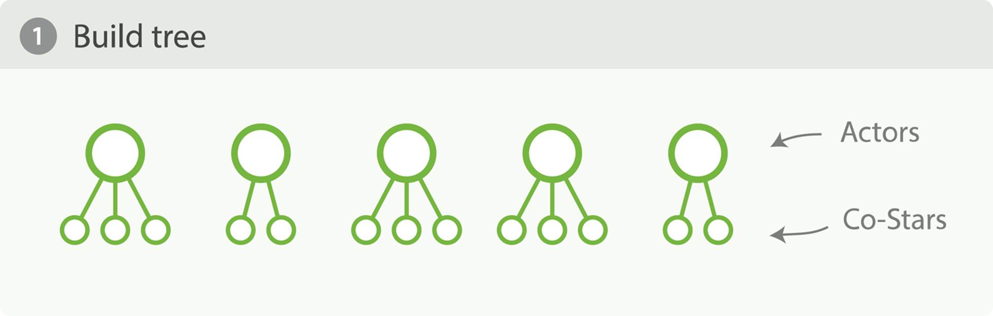
Figure 34-1. Build full depth tree
To use some real numbers, imagine each movie has 10 actors on average. Each movie will then generate 102 == 100 buckets. If you have 20,000 movies, that’s roughly 2,000,000 generated buckets.
Now, remember, our aggregation is simply asking for the top 10 actors and their co-stars, totaling 50 values. To get the final results, we have to generate that tree of 2,000,000 buckets, sort it, and finally prune it such that only the top 10 actors are left. This is illustrated in Figure 34-2 andFigure 34-3.

Figure 34-2. Sort tree

Figure 34-3. Prune tree
At this point you should be quite distraught. Twenty thousand documents is paltry, and the aggregation is pretty tame. What if you had 200 million documents, wanted the top 100 actors and their top 20 costars, as well as the costars’ costars?
You can appreciate how quickly combinatorial expansion can grow, making this strategy untenable. There is not enough memory in the world to support uncontrolled combinatorial explosions.
Depth-First Versus Breadth-First
Elasticsearch allows you to change the collection mode of an aggregation, for exactly this situation. The strategy we outlined previously—building the tree fully and then pruning—is called depth-first and it is the default. Depth-first works well for the majority of aggregations, but can fall apart in situations like our actors and costars example.
For these special cases, you should use an alternative collection strategy called breadth-first. This strategy works a little differently. It executes the first layer of aggregations, and then performs a pruning phase before continuing, as illustrated in Figure 34-4 through Figure 34-6.
In our example, the actors aggregation would be executed first. At this point, we have a single layer in the tree, but we already know who the top 10 actors are! There is no need to keep the other actors since they won’t be in the top 10 anyway.

Figure 34-4. Build first level

Figure 34-5. Sort first level

Figure 34-6. Prune first level
Since we already know the top ten actors, we can safely prune away the rest of the long tail. After pruning, the next layer is populated based on its execution mode, and the process repeats until the aggregation is done, as illustrated in Figure 34-7. This prevents the combinatorial explosion of buckets and drastically reduces memory requirements for classes of queries that are amenable to breadth-first.

Figure 34-7. Populate full depth for remaining nodes
To use breadth-first, simply enable it via the collect parameter:
{
"aggs" : {
"actors" : {
"terms" : {
"field" : "actors",
"size" : 10,
"collect_mode" : "breadth_first" ![]()
},
"aggs" : {
"costars" : {
"terms" : {
"field" : "actors",
"size" : 5
}
}
}
}
}
}
![]()
Enable breadth_first on a per-aggregation basis.
Breadth-first should be used only when you expect more buckets to be generated than documents landing in the buckets. Breadth-first works by caching document data at the bucket level, and then replaying those documents to child aggregations after the pruning phase.
The memory requirement of a breadth-first aggregation is linear to the number of documents in each bucket prior to pruning. For many aggregations, the number of documents in each bucket is very large. Think of a histogram with monthly intervals: you might have thousands or hundreds of thousands of documents per bucket. This makes breadth-first a bad choice, and is why depth-first is the default.
But for the actor example—which generates a large number of buckets, but each bucket has relatively few documents—breadth-first is much more memory efficient, and allows you to build aggregations that would otherwise fail.
All materials on the site are licensed Creative Commons Attribution-Sharealike 3.0 Unported CC BY-SA 3.0 & GNU Free Documentation License (GFDL)
If you are the copyright holder of any material contained on our site and intend to remove it, please contact our site administrator for approval.
© 2016-2026 All site design rights belong to S.Y.A.